Embed Size (px)
Citation preview

A Not So Long Introduction to the Weak Theory of
Parabolic Problems with Singular Data
Lecture Notes of a Course Held in GranadaOctober-December 2007
by
Francesco Petitta

Contents
Chapter 1. Motivations for the problem and basic tools 11.1. Motivations 11.2. Functional spaces involving time 6
Chapter 2. Weak solutions 132.1. Galerkin Method: Existence and uniqueness of a weak solution 14
Chapter 3. Regularity 193.1. Regularity for finite energy solutions 193.2. L1(Q) data 25
Chapter 4. Asymptotic behavior of the solutions 294.1. Naıve idea and main assumptions 29
35
Appendix A. Basic tools in integration and measure theory 35
Bibliography 39
III

IV CONTENTS

CHAPTER 1
Motivations for the problem and basic tools
1.1. Motivations
Here we want to study parabolic equations whose simplest model is theso called (Nonhomogeneous) Heat Equation
ut −∆u = f,
subject to suitable initial and boundary conditions. Here t > 0 and x ∈ Ωwhich is an open subset of RN . The unknown is the function u : Ω×(0, T ) 7→R, where T is a positive, possibly infinity, constant, and ∆ is the usualLaplace Operator with respect to the space variables, that is
∆u =n∑i=1
uxixi ,
while the function f : Ω× (0, T ) 7→ R is a given datum.Historically, the study of parabolic equations followed a parallel path
with respect to the elliptic theory: so many results of the elliptic framework(harmonic properties, maximum principles, representations of solution, . . .)turn out to have a (usually more complicated §) parabolic counterpart.
However, unfortunately (or by chance. . .) the statement Every ellipticproblem becomes parabolic just with time is, in general, false.
On the other hand, a natural question is the reverse one: is it true thatevery parabolic problem turns out to become elliptic with time? We will tryto give an answer to this problem at the end of the last part of the finalclass (If I can. . .).
In any case, the physical interpretation is much more clear and so thesetype of equations turned out to admit many many applications in a widevariety of fields as, among others, Thermodynamics (ca va sans dire. . .),Statistics (Brownian Motion), Fluid Mechanics (Navier-Stokes equations. . .there is a prize about it1), Finance (Black-Scholes equation. . . here there isnot a prize anymore. . . §), an so on.
The heat equation can be considered as diffusion equation and it wasfirstly studied to describe the evolution in time of the density u of somequantity such as heat or chemical concentration. If ω ⊂ Ω is a smooth
1For instance it is still not known if the N-S equation which describes the flow of airaround an airplane has a solution §
1

2 1. MOTIVATIONS FOR THE PROBLEM AND BASIC TOOLS
subregion, the rate of change of the total quantity within ω should equal thenegative of the flux through ∂ω, that is
d
dt
∫ωu dx = −
∫∂ωF · ν dσ,
F being the flux density. Thus,
ut = −divF,
as ω is arbitrary. In many applications F turns out to be proportional to∇u, that leads to ut − λ∆u = 0, that is the Heat Equation for λ = 1;
(1.1) ut −∆u = 0.
Let us explicitly remark that the heat equation involves one derivativewith respect to the time and two with respect to x. Consequently, we caneasily check that, if u solves (1.1), then so does u(λx, λ2t), for λ ∈ R; thisinhomogeneity suggests that the ratio |x|
2
t is important to study this typeof equations and that an explicit radial solution can be searched of the formu(x, t) = v( r
2
t ), where r = |x|, and v is the new unknown.Let us formally motivate the introduction of the so called fundamental
solution for (1.1).It is quicker to search for radial solutions through the invariant scaling
r = |y| = t−12 |x|, which yields, after few calculations to derive the radial
form of (1.1):N
2v +
12rv′ + v′′ +
N − 1r
v′ = 0,
which, multiplying the equation by rN−1, turns out to be equivalent to
(rN−1v′)′ +12
(rNv)′ = 0,
that is,
rN−1v′ +12rNv = a,
for some constant a. Now assuming that we look for solutions vanishing atinfinity with its derivatives we conclude that a = 0. Thus
v′ = −12rv,
and so, finally
v = be−r2
4 , (b > 0).
With a suitable choice of the contants (chosen in such a way that thetotal mass of Φ(x, t) on RN is equal to 1 for every t > 0) we can write theclassic fundamental solution for problem (1.1), that is
(1.2) Φ(x, t) =1
(4πt)N2
e−|x|24t (x ∈ RN , t > 0).

1.1. MOTIVATIONS 3
The fundamental solution can be used to represent solutions for initial-boundary value problems (Cauchy problems) of the type
(1.3)
ut −∆u = 0 in RN × (0,∞)u(x, 0) = g.
In fact the following result holds true
Theorem 1.1. Let g ∈ C(RN ) ∩ L∞(RN ), then
(1.4) u(x, t) =∫
RNΦ(x− y, t)g(y) dy,
belongs to C∞(RN × (0,∞)), solves the equation in (1.3) and
lim(x,t)→(x0,0)
u(x, t) = g(x0), (x0 ∈ RN ).
Proof. [E], p. 47.
If we have a nonhomogeneous smooth forcing term f the representationformula is more complicated (but just a little bit. . .) and involves the socalled superposition Duhamel Principle. In fact, if we assume for simplicityf ∈ C2
1 (RN × [0,∞)) (i.e., two continuous derivatives in space and one intime) with compact support, then the representation formula for the solutionto problem
(1.5)
ut −∆u = f in RN × (0,∞)u(x, 0) = g,
will be
u(x, t) =∫
RNΦ(x− y, t)g(y) dy +
∫ t
0
∫RN
Φ(x− y, t− s)f(y, s) dyds.
Remark 1.2. In view of Theorem 1.1 we sometimes say that the funda-mental solution solves
(1.6)
Φt −∆Φ = 0 in RN × (0,∞)Φ(x, 0) = δ0,
where δ0 denotes the Dirac mass at 0. Notice moreover that, from (1.4), wederive that for nonnegative data g 6= 0 the solution turns out to be strictlypositive for all x ∈ RN , and t > 0. This is a key feature for parabolicsolutions which have the so called infinite propagation speed. If the initialtemperature is nonnegative and positive somewhere, then at any positivetime t the temperature is positive anywhere. This fact turns out to play anessential difference with other types of evolution equations such, for instance,Hyperbolic Equations.
As we said many features of harmonic functions are inherited by solu-tions of the heat equation. For example, the parabolic mean value formula.

4 1. MOTIVATIONS FOR THE PROBLEM AND BASIC TOOLS
Theorem 1.3 (Mean value formula). Let Ω be a smooth, connected,bounded open set of RN , and Q = Ω × (0, T ), T > 0. Assume u ∈ C2
1 (Ω ×(0, T ]) ∩ C(Q) solves the heat equation in Q. Then we have
u(x, t) =1
4rN
∫E(x,t;r)
u(y, s)|x− y|2
(t− s)2dy ds
for every E(x, t; r) ⊂ Q, where
E(x, t; r) =
(y, s) ∈ RN × R : s ≤ t,Φ(x− y, s− t) ≥ 1rN
,
is the so-called heat ball.
Figure 1. The heat ball
Proof. See [E], p. 52.
As for harmonic functions, from the mean value formula a maximumprinciple follows.
Theorem 1.4 (Strong Maximum Principle). Let Ω be a smooth, con-nected, bounded open set of RN , and Q = Ω × (0, T ), T > 0. Assumeu ∈ C2
1 (Ω× (0, T ])∩C(Q) solves the heat equation in Q. Then, if we denoteΓ = Q\(Ω× (0, T ]), we have
i)maxQ
u = maxΓ
u,
ii) If u attains its maximum at (x0, t0) ∈ Q, then u is constant inΩ× [0, t0].
Proof. See [E], p. 54.

1.1. MOTIVATIONS 5
Theorem 1.4 has a very suggestive interpretation: with constant data onthe boundary, the solution keeps itself constant until something happens tochange this quiet status (think about a change of boundary conditions fromt0 on). In some sense, a solution behaves in a very intuitive way since thepast turns out to be independent on the future. This fact is strongly relatedto the irreversibility of the heat equation, that is on the ill-posedness of thefinal-boundary value problem
(1.7)
ut −∆u = 0 in Ω× (0, T )u(x, T ) = g.
Looking for solutions to problem (1.7) is, in some sense, equivalent tofind out an initial datum such that the corresponding solution of the Cauchyproblem coincides with g at time T . However, because of the strong reg-ularization of the solution emphasized by Theorem 1.1, if g is not smoothenough there is no chance to solve (1.7). So this should convince us that theuse of the symbol t to denote the last variable of the unknown u is not justa mere chance.
Of course, once the maximum principle is at hand, uniqueness of thesolution follows by difference:
Theorem 1.5 (Uniqueness on bounded domains). Let g ∈ C(Γ), f ∈C(Q). Then there exists at most one solution u ∈ C2
1 (Q) ∩ C(Q) of theinitial boundary problem for the heat equation.
Proof. See [E], p. 57.
What happens if the domain is unbounded, for example is the wholeRN? In this case uniqueness is no longer true, but we can recover it (as wellas the maximum principle), by adding a suitable control on the solution forlarge |x|.
Theorem 1.6 (Maximum principle in unbounded domains). If u is asolution of the heat equation in RN × (0, T ) (with initial datum g), and u issuch that
(1.8) u(x, t) ≤ A ea|x|2,
for some constants A > 0 and a > 0, then
supRN×[0,T ]
u(x, t) = supRN
g(x).
Proof. See [E], p. 57.
This maximum principle then implies as before the uniqueness of thesolutions of the Cauchy problem in the class of functions whose absolutevalue satisfies (1.8).

6 1. MOTIVATIONS FOR THE PROBLEM AND BASIC TOOLS
Notation and remarks. Let us spend a few words on how positiveconstant will be denoted hereafter. If no otherwise specified, we will writeC to denote any positive constant (possibly different) which only dependson the data, that is on quantities that are fixed in the assumptions (N ,Ω, Q, p, and so on. . . ). In any case such constants never depend on thedifferent indexes having a limit we often introduce. Finally, for the sakeof simplification of the notation we will indicate the time derivative of afunction u with ut, du
dt or u′ depending on the context.For the convenience of the reader in Appendix A we recall some basic
results of measure and integration theory we will always assume to be knownin the following.
1.2. Functional spaces involving time
Since we want to study an equation involving one derivative in time andtwo in space, the right functional setting should be C1 in time and C2 inspace, and, in fact, this is the classical setting we mentioned above.
However, as in the elliptic case, we would like to solve problems withless regular data. Due to this fact, we will deal with the weak theory ofparabolic problems, so that, to our aims, it would be sufficient a functionalsetting involving zero derivatives in time (Lebesgue regularity) and just onein space (Sobolev regularity).
Let us just recall that, if E and F are Banach spaces,then the function
f : E → Fx 7→ f(x),
is said to be Frechet differentiable at a ∈ E, if there exist a linear boundedmap D from E to F such that
lim‖h‖E→0
‖f(a+ h)− f(a)−Da(h)‖F‖h‖E
= 0.
Given a real Banach space V , we will denote by C∞(R;V ) the space offunctions u : R → V which are infinitely many times Frechet differentiableand by C∞0 (R;V ) the space of functions in C∞(R;V ) having compact sup-port. As we mentioned above, for a, b ∈ R, C∞([a, b];V ) will be the space ofthe restrictions to [a, b] of functions of C∞0 (R;V ), and C([a, b];V ) the spaceof all continuous functions from [a, b] into V .
We recall that a function u : [a, b]→ V is said to be Lebesgue measurable
if there exists a sequence un of step functions (i.e. un =kn∑j=1
anj χAnj for a
finite number kn of Borel subsets Anj ⊂ [a, b] and with anj ∈ V ) convergingto u almost everywhere with respect to the Lebesgue measure in [a, b].

1.2. FUNCTIONAL SPACES INVOLVING TIME 7
Then for 1 ≤ p < ∞, Lp(a, b;V ) is the space of measurable functionsu : [a, b]→ V such that
‖u‖Lp(a,b;V ) =(∫ b
a‖u‖pV dt
) 1p
<∞,
while L∞(a, b;V ) is the space of measurable functions such that:
‖u‖L∞(a,b;V ) = sup[a,b]‖u‖V <∞.
Of course both spaces are meant to be quotiented, as usual, with respect tothe almost everywhere equivalence. The reader can find a presentation ofthese topics in [DL].
Let us recall that, for 1 ≤ p ≤ ∞, Lp(a, b;V ) is a Banach space. More-over, for 1 ≤ p < ∞ and if the dual space V ′ of V is separable, then thedual space of Lp(a, b;V ) can be identified with Lp
′(a, b;V ′).
For our purpose V will mainly be either the Lebesgue space Lp(Ω) orthe Sobolev space W 1,p
0 (Ω), with 1 ≤ p <∞ and Ω will be a bounded openset of RN . Since, in this case, V is separable, we have that Lp(a, b;Lp(Ω)) =Lp((a, b) × Ω)), the ordinary Lebesgue space defined in (a, b) × Ω. Notethat Lp(a, b;W 1,p
0 (Ω)) consists of all functions u : [a, b] × Ω → R whichbelong to Lp((a, b) × Ω)) and such that ∇u = (ux1 , . . . , uxN ) belongs to(Lp((a, b)× Ω))N . Moreover,(∫ b
a
∫Ω|∇u|p dxdt
) 1p
defines an equivalent norm by Poincare inequality.Given a function u in Lp(a, b;V ) it is possible to define a time derivative
of u in the space of vector valued distributions D′(a, b;V ) which is the spaceof linear continuous functions from C∞0 (a, b) into V (see [Sc] for furtherdetails). In fact, the definition is the following:
〈ut, ψ〉 = −∫ b
auψt dt , ∀ ψ ∈ C∞0 (a, b),
where the equality is meant in V . If u ∈ C1(a, b;V ) this definition clearlycoincides with the Frechet derivative of u. In the following, ut is said tobelong to a space Lq(a, b; V ) (V being a Banach space) if there exists afunction z ∈ Lq(a, b; V ) ∩ D′(a, b;V ) such that:
〈ut, ψ〉 = −∫ b
auψt dt = 〈z, ψ〉 , ∀ ψ ∈ C∞0 (a, b).
In the following, we will also use sometimes the notation∂u
∂tinstead of ut.
We recall the following classical embedding result

8 1. MOTIVATIONS FOR THE PROBLEM AND BASIC TOOLS
Theorem 1.7. Let H be an Hilbert space such that:
V →dense
H → V ′ .
x Let u ∈ Lp(a, b;V ) be such that ut, defined as above in the distributionalsense, belongs to Lp
′(a, b;V ′). Then u belongs to C([a, b];H).
Sketch of the proof. We give a sketch of the proof of this result inthe particular case p = 2 and V = H1
0 (Ω) (in this case the pivot space Hwill be L2(Ω)). A complete proof of Theorem 1.7 can be found in [DL]. forsimplicity we also choose a = 0, and b = T .
Extend u to the larger interval [−σ, T + σ], for σ > 0, and define theregularizations uε = ηε ∗ u, where ηε is a mollifier on R. One can easilycheck that,
(1.9)
uε → u in L2(0, T ;H1
0 (Ω)),uεt → ut in L2(0, T ;H−1(Ω)).
Then, for ε, δ > 0,d
dt‖uε(t)− uδ(t)‖2L2(Ω) = 2〈uεt (t)− uδt (t), uε(t)− uδ(t)〉L2(Ω).
Thus, integrating between s and t we have
(1.10)
‖uε(t)− uδ(t)‖2L2(Ω) = ‖uε(s)− uδ(s)‖2L2(Ω)
+2∫ t
s〈uεt (τ)− uδt (τ), uε(τ)− uδ(τ)〉L2(Ω) dτ ,
for all 0 ≤ s, t ≤ T . Now, as a consequence of (1.9), for a.e. s ∈ (0, T ), wehave
uε(s) −→ u(s) in L2(Ω).So that, for these s, from (1.10), using both Cauchy-Schwartz and Young’sinequality, we can write
sup0≤t≤T
‖uε(t)− uδ(t)‖2L2(Ω) ≤ ‖uε(s)− uδ(s)‖2L2(Ω)
+∫ T
0‖uεt (τ)− uδt (τ)‖2H−1(Ω) + ‖uε(τ)− uδ(τ)‖2H1
0 (Ω) dτ = ω(ε, δ),
thanks to (1.9) (here ω(ε, δ) tends to zero as ε and δ tend to zero).So uε converges to a function v in C([0, T ];L2(Ω)); since we know that
uε(t)→ u(t) for a.e. t, we deduce that v = u a.e.
This result also allows us to deduce, for functions u and v enjoying theseproperties, the integration by parts formula:
(1.11)∫ b
a〈v, ut〉 dt+
∫ b
a〈u, vt〉 dt = (u(b), v(b))− (u(a), v(a)) ,

1.2. FUNCTIONAL SPACES INVOLVING TIME 9
where 〈·, ·〉 is the duality between V and V ′ and (·, ·) the scalar product in H.Notice that the terms appearing in (1.11) make sense thanks to Theorem 1.7.The proof of (1.11) relies on the fact that C∞0 (a, b;V ) is dense in the spaceof functions u ∈ Lp(a, b;V ) such that ut ∈ Lp
′(a, b;V ′) endowed with the
norm ‖u‖ = ‖u‖Lp(a,b;V ) + ‖ut‖Lp′ (a,b;V ′), together with the fact that (1.11)is true for u, v ∈ C∞0 (a, b;V ) by the theory of integration and derivation inBanach spaces. Note however that in this context (1.11) is subject to thesatisfication of the hypotheses of Theorem 1.7; if, for instance, V = W 1,p
0 (Ω),then
W 1,p0 (Ω) →
denseL2(Ω) →W−1,p′(Ω)
only if p ≥ 2NN+2 ; for the sake of simplicity we will often work under this
bound, that actually turns out to be only technical to our purposes.
1.2.1. Further useful results. Here we give some further results thatwill be very useful in what follows; the first one contains a generalizationof the integration by parts formula (1.11) where the time derivative of afunction is less regular than there; its proof can be found in [DP] (see also[CW]).
Lemma 1.8. Let f : R→ R be a continuous piecewise C1 function suchthat f(0) = 0 and f ′ is compactly supported on R; let us denote F (s) =∫ s
0 f(r)dr. If u ∈ Lp(0, T ;W 1,p0 (Ω)) is such that ut ∈ Lp
′(0, T ;W−1,p′(Ω)) +
L1(Q) and if ψ ∈ C∞(Q), then we have
(1.12)
∫ T
0〈ut, f(u)ψ〉 dt =
∫ΩF (u(T ))ψ(T ) dx
−∫
ΩF (u(0))ψ(0) dx−
∫Qψt F (u) dxdt.
Now we state three embedding theorems that will play a central rolein our work; the first one is the well-known Gagliardo-Nirenberg embeddingtheorem followed by an important consequence of it for the evolution case,while the second one is an Aubin-Simon type result that we state in a formgeneral enough to our purpose; the third one is a useful generalization ofTheorem 1.7.
Theorem 1.9 (Gagliardo-Nirenberg). Let v be a function in W 1,q0 (Ω)∩
Lρ(Ω) with q ≥ 1, ρ ≥ 1. Then there exists a positive constant C, dependingon N , q and ρ, such that
‖v‖Lγ(Ω) ≤ C‖∇v‖θ(Lq(Ω))N ‖v‖1−θLρ(Ω) ,
for every θ and γ satisfying
0 ≤ θ ≤ 1, 1 ≤ γ ≤ +∞, 1γ
= θ
(1q− 1N
)+
1− θρ
.
Proof. See [N], Lecture II.

10 1. MOTIVATIONS FOR THE PROBLEM AND BASIC TOOLS
A consequence of the previous result is the following embedding result:
Corollary 1.10. Let v ∈ Lq(0, T ;W 1,q0 (Ω)) ∩ L∞(0, T ;Lρ(Ω)), with
q ≥ 1, ρ ≥ 1. Then v ∈ Lσ(Q) with σ = qN+ρN and
(1.13)∫Q|v|σ dxdt ≤ C‖v‖
ρqN
L∞(0,T ;Lρ(Ω))
∫Q|∇v|q dxdt .
Proof. By virtue of Theorem 1.9, we can write∫Ω|v|σ ≤ C ‖∇v‖ϑσLq(Ω) ‖v‖
(1−ϑ)σLρ(Ω) ,
that is, integrating between 0 and T
(1.14)∫ T
0
∫Ω|v|σ ≤ C
∫ T
0‖∇v(t)‖ϑσLq(Ω) ‖v(t)‖(1−ϑ)σ
Lρ(Ω) dt,
now, since v ∈ Lq(0, T ;W 1,q0 (Ω)) ∩ L∞(0, T ;Lρ(Ω)), we have∫ T
0
∫Ω|v|σ ≤ C ‖v‖(1−ϑ)σ
L∞((0,T );Lρ(Ω))
∫ T
0‖∇v(t)‖σϑLq(Ω) dt.
Now we choose
ϑ =q
σ=
N
N + ρ
so thatσϑ = q, (1− ϑ)σ =
qρ
N,
and (1.14) becomes∫ T
0
∫Ω|v|σ ≤ C ‖v‖
qρN
L∞((0,T );Lρ(Ω))
∫ T
0‖∇v(t)‖qLq(Ω) dt,
that is ∫Q|v|σ ≤ C ‖v‖
qρN
L∞((0,T );Lρ(Ω))
∫Q|∇v|q .
Remark 1.11. Let us explicitly remark that Corollary 1.10 gives us alittle gain on the a priori summability of the involved function (actually thisis a consequence of the Gagliardo-Nirenberg inequality, not a consequenceof a Petitta’s inequality ©). As an example, let us think about a functionu ∈ L∞(0, T ;L2(Ω)) ∩ L2(0, T ;H1
0 (Ω)); in this case the solution turns outto belong to L2+ 4
N (Q).
Theorem 1.12. Let un be a sequence bounded in Lq(0, T ;W 1,q0 (Ω)) such
that unt is bounded in L1(Q) + Ls′(0, T ;W−1,s′(Ω)) with q, s > 1, then un is
relatively strongly compact in L1(Q), that is, up to subsequences, un stronglyconverges in L1(Q) to some function u.
Proof. See [Si], Corollary 4.

1.2. FUNCTIONAL SPACES INVOLVING TIME 11
Let us define, for every p > 1, the space Sp as
(1.15) Sp = u ∈ Lp(0, T ;W 1,p0 (Ω));ut ∈ L1(Q) + Lp
′(0, T ;W−1,p′(Ω)),
endowed with its natural norm
‖u‖Sp = ‖u‖Lp(0,T ;W 1,p
0 (Ω))+ ‖ut‖Lp′ (0,T ;W−1,p′ (Ω))+L1(Q).
We have the following trace result:
Theorem 1.13. Let p > 1, then we have the following continuous injec-tion
Sp → C(0, T ;L1(Ω)).
Proof. See [Po], Theorem 1.1.


CHAPTER 2
Weak solutions
Let Ω ⊆ RN be a bounded open set, N ≥ 2, t > 0; we denote by Qt thecylinder Ω × (0, t). If t = T we will often write Q for QT . In this chapterwe are interested in the study existence, uniqueness, and regularity of thesolution of the linear parabolic problem
(2.1)
ut + L(u) = f in Ω× (0, T ),u(0) = u0, in Ω,u = 0 on ∂Ω× (0, T ),
where
L(u) = −div(A(x, t)∇u),
and A is a matrix with bounded, measurable entries, such that
(2.2) |A(x, t)ξ| ≤ β|ξ|,
for any ξ ∈ RN , with β > 0, and
(2.3) A(x, t)ξ · ξ ≥ α|ξ|2,
for any ξ ∈ RN , with α > 0. As we will see such results strongly depend onthe regularity of the data f , u0 and A.
We first deal existence, uniqueness and (weak) regularity for linear prob-lems in the framework of Hilbert spaces, that is f ∈ L2(0, T ;H−1(Ω)) andu0 ∈ H1
0 (Ω). For such data the solution is supposed to be in the spaceL∞(0, T ;L2(Ω)) ∩ L2(0, T ;H1
0 (Ω)), with ut ∈ L2(0, T ;H−1(Ω)). Moreover,we expect the solutions to belong to C(0, T ;L2(Ω)) to give sense at theinitial value u0.
Indeed if we formally multiply the equation in (2.1) by u and using (2.3),integrating on Ω and between 0 and t (here 0 < t ≤ T ), we obtain, usingalso Young’s inequality,∫ t
0〈ut, u〉+ α
∫Q|∇u|2 ≤
∫ t
0‖f‖H−1(Ω)‖u‖H1
0 (Ω)
≤ ‖f‖L2(0,T ;H−1(Ω))‖u‖L2(0,T ;H10 (Ω))
≤ 12α‖f‖2L2(0,T ;H−1(Ω)) +
α
2‖u‖2L2(0,T ;H1
0 (Ω)).
13
14 2. WEAK SOLUTIONS
Which, thanks to the fact that∫ t
0〈ut, u〉 =
∫ t
0
12d
dtu2,
using (1.11) yields
12
∫Ωu2(t) +
α
2
∫Qt
|∇u|2 ≤ C(‖f‖2L2(0,T ;H−1(Ω)) + ‖u0‖2L2(Ω)).
Now, since the right hand side does not depend on t we easily deduce thatthe same inequality holds true for any 0 ≤ t ≤ T , and so
(2.4)
12‖u‖2L∞(0,T ;L2(Ω)) +
α
2‖u‖2L2(0,T ;H1
0 (Ω))
≤ C(‖f‖2L2(0,T ;H−1(Ω)) + ‖u0‖2L2(Ω)),
which thanks to Theorem 1.7 it gives the desired regularity result.The energy estimates can also be useful to prove the so-called backward
uniqueness.
Theorem 2.1 (Backward uniqueness). Let u and u be two solutions inQ such that u(x, T ) = u(x, T ). Then u = u in Q.
Proof. See [E], p. 64.
Remark 2.2. Let us stress the fact that, as a difference with the ellipticcase, here it is not so easy to face the problem with a Lax-Milgram typeapproach (or with minimizing some functional) because of the features ofthe involved functional spaces and of the operator itself. Indeed, roughlyspeaking, the supposed involved bilinear form would turn out to be, forinstance, not continuous on L2(0, T ;H1
0 (Ω)), not coercive on
W = u ∈ L2(0, T ;H10 (Ω)), ut ∈ L2(0, T ;H−1(Ω)),
and L2(0, T ;H10 (Ω)) ∩ L∞(0, T ;L2(Ω)) is not an Hilbert space.
2.1. Galerkin Method: Existence and uniqueness of a weaksolution
Let us first give our definition for weak solutions to problem (2.1)
Definition 2.3. We say that a function u ∈ L2(0, T ;H10 (Ω)), such that
ut ∈ L2(0, T ;H−1(Ω)) is a weak solution for problem (2.1) if(2.5)∫ T
0〈u′, ϕ〉H−1(Ω),H1
0 (Ω)+∫QA(x, t)∇u·∇ϕ = 〈f, ϕ〉L2(0,T ;H−1(Ω)),L2(0,T ;H1
0 (Ω)),
for all ϕ ∈ L2(0, T ;H10 (Ω)) such that ϕt ∈ L2(0, T ;H−1(Ω)), ϕ(T ) = 0, and
u(x, 0) = u0 in the sense of L2(Ω).
2.1. GALERKIN METHOD: EXISTENCE AND UNIQUENESS OF A WEAK SOLUTION15
Remark 2.4. Observe that, taking into account Theorem 1.7, we caneasily see that all terms in Definition 2.3 turn out to make sense.
Moreover, as shown in [E] (actually it is not so difficult to check), iff ∈ L2(Q), u is a weak solution for problem (2.1) if and only if
(2.6) 〈u′(t), v〉H−1(Ω),H10 (Ω) +
∫ΩA(x, t)∇u(t)∇v =
∫Ωf(t)v,
for any v ∈ H10 (Ω) and a.e. in 0 ≤ t ≤ T , with u(0) = u0. We will often
denote by 〈·, ·〉 the duality product between H−1(Ω) and H10 (Ω), while (·, ·)
will be occasionally used to indicate the inner product in L2(Ω).
Now we state our first existence and uniqueness result. Here, for thesake of simplicity, we choose f ∈ L2(Q). We will use the so called GalerkinMethod which relies on the approximation of our problem by mean of fi-nite dimensional problems. For another possible approach, based on theHille-Yosida theorem and on the fact that the Laplace operator is maximalmonotone, see [B], Chapters 7 and 10.
Theorem 2.5. Let f ∈ L2(Q), and u0 ∈ L2(Ω). Then there exists aunique weak solution for problem (2.1).
Proof. We will consider a sequence of functions wk(x), (k = 1, . . .)which satisfy
i) wk is an orthogonal basis of H10 (Ω),
ii) wk is an orthonormal basis of L2(Ω).Observe that the construction of such a sequence is always possible; as anexample (see [E]) we can take wk(x) as a sequence for −∆ in H1
0 (Ω) (aftera suitable normalization).
Fix now an integer m. We will look for a function um : [0, T ] 7→ H10 (Ω)
of the form
(2.7) um(t) =m∑k=1
dkm(t)wk,
and we want to select the coefficients such that
(2.8) dkm(0) = (u0, wk) (k = 1, . . . ,m)
and
(2.9) (u′m, wk) +∫
ΩA(x, t)∇um · ∇wk = (f, wk),
a.e. on 0 ≤ t ≤ T , k = 1, . . . ,m. In other words, we look for the solutionsof the projections of problem (2.1) to the finite dimensional subspaces ofH1
0 (Ω) spanned by wk(k = 1, . . . ,m).During this proof, for the convenience of the reader we will use the
following notation
a(ψ,ϕ, t) ≡∫
ΩA(x, t)∇ψ · ∇ϕ.

16 2. WEAK SOLUTIONS
We split the proof of this result in four steps.Step 1. Construction of approximate solutions.Assume that um has the structure (2.7); since wk is orthonormal in
L2(Ω), then
(u′m, wk) =d
dtdkm(t),
and
a(um, wk, t) =m∑l=1
ekl(t)dlm(t),
where ekl(t) = a(wl, wk, t)(k, l = 1, . . . ,m). Finally, if fk = (f(t), wk) is theprojection of the datum f , then (2.9) becomes the linear system of ODE
d
dtdkm(t) +
m∑l=1
ekl(t)dlm(t) = fk(t),
for k = 1, . . . ,m, subject to the initial condition (2.8). According to thestandard existence theory for ordinary differential equations, there exists aunique absolutely continuous function dm(t) = (dlm, . . . , d
lm) satisfying (2.8)
and the ODE for a.e. 0 ≤ t ≤ T . Then um is the desired approximatesolution since it turns out to solve (2.9).
Step 2. Energy Estimates.Multiply the equation (2.9) by dkm(t) and sum over k between 1 and
m. Then, integrating between 0 and T , we find, recalling that (u′m, um) =12ddtu
2m, and using (2.3)
12
∫ T
0
d
dt
∫Ωu2m + α
∫Q|∇um|2 ≤
∫Qfum.
Thus, reasoning as in the proof of (2.4) we can check that
(2.10) ‖um‖2L∞(0,T ;L2(Ω)) + ‖um‖2L2(0,T ;H10 (Ω)) ≤ C(‖f‖2L2(Q) + ‖u0‖2L2(Ω)),
(here we also used that ‖um(0)‖L2(Ω) ≤ ‖u0‖L2(Ω)).Finally, using the fact that wk is an orthogonal basis in H1
0 (Ω), we canfix any v ∈ H1
0 (Ω) such that ‖v‖H10 (Ω) ≤ 1, and deduce from the equation
(2.9), after a few easy calculations
|〈u′m, v〉| ≤ C(‖f‖L2(Ω) + ‖um‖H10 (Ω)),
that is‖u′m‖H−1(Ω) ≤ C(‖f‖L2(Ω) + ‖um‖H1
0 (Ω)),
whose square integrated between 0 and T , gathered together with (2.10),yields
(2.11) ‖u′m‖2L2(0,T ;H−1(Ω)) ≤ C(‖f‖2L2(Q) + ‖u0‖2L2(Ω)).
Step 3. Existence of a solution.From (2.10) we deduce that there exists a function u ∈ L2(0, T ;H1
0 (Ω)),such that um converges weakly to u in L2(0, T ;H1
0 (Ω)); moreover u′m weakly

2.1. GALERKIN METHOD: EXISTENCE AND UNIQUENESS OF A WEAK SOLUTION17
converges to some function η in L2(0, T ;H−1(Ω)) (one can easily check byusing its definition that η = u′). Then, we can pass to the limit in the weakformulation of um, that is in(2.12)∫ T
0〈u′m, ϕ〉H−1(Ω),H1
0 (Ω)+∫QA(x, t)∇um·∇ϕ = 〈f, ϕ〉L2(0,T ;H−1(Ω)),L2(0,T ;H1
0 (Ω)).
for any ϕ ∈ L2(0, T ;H10 (Ω)), such that ϕ′ ∈ L2(0, T ;H−1(Ω)), with ϕ(T ) =
0, to obtain (2.5).To check that the initial value is achieved we use (1.11) in (2.5) and
(2.12), obtaining respectively
−∫ T
0〈ϕ′, u〉H−1(Ω),H1
0 (Ω) −∫
Ωu(0)ϕ(0) +
∫QA(x, t)∇u · ∇ϕ =
∫Qfϕ,
and
−∫ T
0〈ϕ′, um〉H−1(Ω),H1
0 (Ω) −∫
Ωum(0)ϕ(0) +
∫QA(x, t)∇um · ∇ϕ =
∫Qfϕ.
Now, since um(0) → u0 in L2(Ω), and ϕ(0) is arbitrary we conclude thatu0 = u(0).
Step 4. Uniqueness of the solution.Let u and v be two solutions of problem (2.1) in the sense of Definition
2.3; if we take u− v as test function in the weak formulation for both u andv (by a density argument we can see that this function can be chosen as testin (2.5) even if it does not satisfy, a priori, (u− v)(T ) = 0). By subtracting,using that (u− v)(0) = 0, we obtain
12
∫Ω|u− v|2(T ) +
∫Q|∇(u− v)|2 ≤ 0,
that implies u = v a.e. in Q.


CHAPTER 3
Regularity
3.1. Regularity for finite energy solutions
In this section, we will be concerned with regularity and existence resultsfor solutions of parabolic problem (2.1).
Let us state a first improvement on the regularity of such solutions.
Theorem 3.1 (Improved regularity). Let u0 ∈ H10 (Ω) and f ∈ L2(Q).
Then the weak solution u of (2.1) satisfies
u ∈ L2(0, T ;H2(Ω)) ∩ L∞(0, T ;H10 (Ω)), u′ ∈ L2(Q),
with continuous estimates with respect to the data.
Proof. [E], Theorem 5, pag. 360.
The previous statement gives a first standard regularity result in theHilbertian case, but what happens if we know something more (or somethingless) on the datum f? For instance, what is the best Lebesgue space whichthe solution turns out to belong to?
We will prove the following
Theorem 3.2. Assume (2.2), (2.3), u0 ∈ L2(Ω), and let f belong toLr(0, T ;Lq(Ω)) with r and q belonging to [1,+∞] and such that
(3.13)1r
+N
2q< 1 .
Then there exists a weak solution of (2.1) belonging to L∞(Q). Moreoverthere exists a positive constant d, depending only from the data (and henceindependent on u), such that
(3.14) ‖u‖L∞(Q) ≤ d.
Notice that assumption (3.13) implies that r ∈ (1,+∞] and q ∈(N2 ,+∞
].
To give an idea, let us represent the summability of the datum f ∈Lr(0, T ;Lq(Ω)) in a diagram with axes
1q
and1r
. Since r, q ∈ [1,+∞], then
all the possible cases of summability are inside of the square [0, 1] × [0, 1]
(we use the notation1∞
= 0).
19

20 3. REGULARITY
If f belongs to Lr(0, T ;Lq(Ω)) where r and q are large enough, that is,if
(3.15)1r
+N
2q< 1 (zone 1 in Figure 1 below),
then every weak solution u belonging to
V2(Q) ≡ L∞(0, T ;L2(Ω)) ∩ L2(0, T ;H10 (Ω))
belongs also to L∞(Q) (see Theorem 3.2 above). This fact was proved byAronson and Serrin in the nonlinear case (see [AS]), while can be found inthe linear setting in some earlier papers as, among the others, [LU] and [A].
Figure 1. Classical regularity results.
In order to prove that the solutions of (2.1) are bounded when thesummability exponents of f are in the zone 1 in the figure 1, we enunci-ate a very well known lemma due to Guido Stampacchia ([S]).
Lemma 3.3. Let us suppose that ϕ is a real, nonnegative and nonin-creasing function satisfying
(3.16) ϕ(h) ≤ C
(h− k)δ[ϕ(k)]ν ∀ h > k > k0,
where C and δ are positive constants and ν > 1. Then there exists a positiveconstant d such that
ϕ(k0 + d) = 0.
Let us give the proof of Theorem 3.2
Proof of Theorem 3.2. For the sake of simplicity, we will restrictourselves to the case u0 = 0, f ≥ 0 and r = q, so that the solution u isnonnegative thanks to the maximum principle, and
q >N
2+ 1 =
N + 22
.
For k > 0, define
(3.17) Ak = (x, t) ∈ Q : u(x, s) > k,

3.1. REGULARITY FOR FINITE ENERGY SOLUTIONS 21
and take Gk(u) as a test function in (2.1), where Gk(s) = (s − k)+. Inte-grating in (0, t]× Ω, where t ≤ T , and using assumption (2.3) we get
12
∫ΩGk(u)2(t)dx+ α
∫ t
0
∫Ω|∇Gk(u)|2dxdt ≤
∫Qt
fGk(u)dxdt.
Taking the supremum for t ∈ (0, T ] on the right, we have (since both f andGk(u) are nonnegative)
12
∫ΩGk(u)2(t)dx+ α
∫ t
0
∫Ω|∇Gk(u)|2dxdt ≤
∫QfGk(u)dxdt,
which implies12
∫ΩGk(u)2(t)dx ≤
∫QfGk(u)dxdt,
andα
∫Qt
|∇Gk(u)|2dxdt ≤∫QfGk(u)dxdt.
Taking the supremum on t in (0, T ] on the left, and summing up, we thereforeget
(3.18) C0
[‖Gk(u)‖2L∞(0,T ;L2(Ω)) + ‖∇Gk(u)‖2L2(Q)
]≤∫QfGk(u) dx dt.
By Corollary 1.10, since∫QGk(u)2N+2
N dx dt ≤ ‖Gk(u)‖4N
L∞(0,T ;L2(Ω))‖∇Gk(u)‖2L2(Q),
we have ∫QGk(u)2N+2
N dx dt ≤ C(∫
QfGk(u)
)N+2N
Using Holder inequality with exponents 2N+2N and 2N+4
N+4 , and observing thatboth integrals are on Ak, we have∫Ak
Gk(u)2N+2N dx dt ≤ C
(∫Ak
f2N+4N+4 dx dt
)N+42N(∫
Ak
Gk(u)2N+2N dx dt
) 12
,
from which it follows∫Ak
Gk(u)2N+2N dx dt ≤ C
(∫Ak
f2N+4N+4 dx dt
)N+4N
.
Since q > N+22 > 2N+4
N+4 , a further use of the Holder inequality yields∫Ak
Gk(u)2N+2N dx dt ≤ C ‖f‖
2(N+2)Nq
Lq(Q) meas(Ak)N+4N− 2(N+2)
Nq .
If h > k > 0, we then deduce, since Gk(u) ≥ h− k on Ah ⊆ Ak,
meas(Ah) (h− k)2N+2N ≤
∫Ak
Gk(u)2N+2N dx dt ≤ C meas(Ak)
N+4N− 2(N+2)
Nq .

22 3. REGULARITY
Setting ϕ(h) = meas(Ah) we then have
ϕ(h) ≤ C
(h− k)2N+2N
ϕ(k)N+4N− 2(N+2)
Nq .
If q > N+22 we can apply Lemma 3.3, to conclude that there exists a constant
d, depending only on q, ‖f‖Lq(Q) and α, such that ϕ(d) = 0, that is
‖u‖L∞(Q) ≤ d.
What happens if r and q do not satisfy (3.15) but satisfy
(3.19) 2 <2r
+N
q≤ min
2 +
N
r, 2 +
N
2
, r ≥ 1 ,
that is, zone 2 and 3 in Figure 1? Ladyzenskaja, Solonnikov and Ural’ceva(see Theorem 9.1, cap. 3 in [LSU]) proved that any weak solution of (2.1)belonging to V2(Q) satisfies also
(3.20) |u(x, t)|γ ∈ V2(Q),
where γ is a constant greater than one that is given by an explicit formulain terms of N , r and q. This value of γ and Theorem 1.10 will then implythat
(3.21) u ∈ Ls(Q), s =(N + 2)qr
Nr + 2q − 2qrA natural question that arises is whether there exists at least a solution
of (2.1) belonging to V2(Q) if the summability exponents (r, q) of f satisfy(3.19).
If (3.19) holds with r ≥ 2 (zone 3 in Figure 1) then the function fbelongs also to the space L2(0, T ;H−1(Ω)), so that it is very easy to deducethe existence of at least such a weak solution.
If otherwise (3.19) holds with r < 2 (zone 2 in Figure 1) then f doesnot belong to L2(0, T ;L(2∗)′(Ω)), but again there exists at least a solutionof (2.1) belonging to V2(Q) as proved in [LSU] for linear operators (see[BDGO] for more general nonlinear operators).
Indeed in [LSU] (Theorem 4.1 cap. 3) it is proved the previous existenceresult when the summability exponent of f satisfies
1r
+N
2q= 1 +
N
4q ∈
[2NN + 2
, 2], r ∈ [1, 2],
but this implies that the result is true for every choice of exponents (r, q)satisfying
(3.22)1r
+N
2q≤ 1 +
N
4, q ≥ 2N
N + 2,
see zones 2, 3 and 4 in Figure 2.
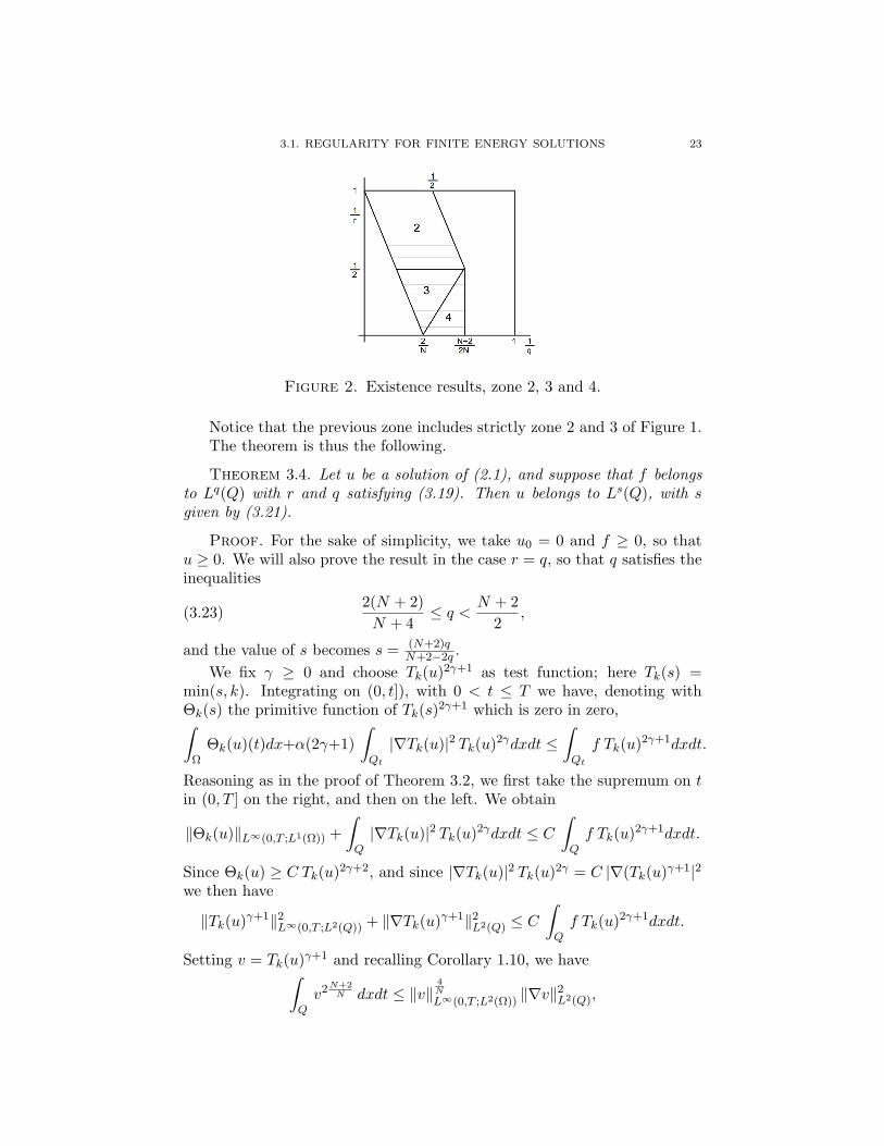
3.1. REGULARITY FOR FINITE ENERGY SOLUTIONS 23
Figure 2. Existence results, zone 2, 3 and 4.
Notice that the previous zone includes strictly zone 2 and 3 of Figure 1.The theorem is thus the following.
Theorem 3.4. Let u be a solution of (2.1), and suppose that f belongsto Lq(Q) with r and q satisfying (3.19). Then u belongs to Ls(Q), with sgiven by (3.21).
Proof. For the sake of simplicity, we take u0 = 0 and f ≥ 0, so thatu ≥ 0. We will also prove the result in the case r = q, so that q satisfies theinequalities
(3.23)2(N + 2)N + 4
≤ q < N + 22
,
and the value of s becomes s = (N+2)qN+2−2q .
We fix γ ≥ 0 and choose Tk(u)2γ+1 as test function; here Tk(s) =min(s, k). Integrating on (0, t]), with 0 < t ≤ T we have, denoting withΘk(s) the primitive function of Tk(s)2γ+1 which is zero in zero,∫
ΩΘk(u)(t)dx+α(2γ+1)
∫Qt
|∇Tk(u)|2 Tk(u)2γdxdt ≤∫Qt
f Tk(u)2γ+1dxdt.
Reasoning as in the proof of Theorem 3.2, we first take the supremum on tin (0, T ] on the right, and then on the left. We obtain
‖Θk(u)‖L∞(0,T ;L1(Ω)) +∫Q|∇Tk(u)|2 Tk(u)2γdxdt ≤ C
∫Qf Tk(u)2γ+1dxdt.
Since Θk(u) ≥ C Tk(u)2γ+2, and since |∇Tk(u)|2 Tk(u)2γ = C |∇(Tk(u)γ+1|2we then have
‖Tk(u)γ+1‖2L∞(0,T ;L2(Q)) + ‖∇Tk(u)γ+1‖2L2(Q) ≤ C∫Qf Tk(u)2γ+1dxdt.
Setting v = Tk(u)γ+1 and recalling Corollary 1.10, we have∫Qv2N+2
N dxdt ≤ ‖v‖4N
L∞(0,T ;L2(Ω))‖∇v‖2L2(Q),

24 3. REGULARITY
from which it follows∫Qv2N+2
N dxdt ≤ C(∫
Qf v
2γ+1γ+1 dxdt
)N+2N
.
Recalling that f belongs to Lq(Q) and using Holder inequality, we obtain∫Qv2N+2
N dxdt ≤ C ‖f‖N+2N
Lq(Q)
(∫Qvq′ 2γ+1γ+1 dxdt
)N+2Nq′
.
We now choose γ such that
q′2γ + 1γ + 1
= 2N + 2N
,
that is
γ + 1 =Nq
2(N + 2− 2q).
The condition γ ≥ 0 is satisfied if and only if
2(N + 2)N + 4
≤ q < N + 22
,
which is true by (3.23). Since q < N+22 , the exponent N+2
Nq′ is smaller than 1,so that we obtain (∫
Qv2N+2
N dxdt
)1−N+2Nq′
≤ C ‖f‖N+2N
Lq(Q).
Recalling the definition of v, and the choice of γ, we then have(∫QTk(u)
(N+2)qN+2−2q dxdt
)1−N+2Nq′
≤ C ‖f‖N+2N
Lq(Q).
Letting k tend to infinity we then have, by Fatou lemma,
‖u‖N+2N
Ls(Q) ≤ C ‖f‖N+2N
Lq(Q),
with s = (N+2)qN+2−2q , as desired.
What happens in the remaining zone (i.e., zone 4 in Figure 2) where, as justsaid, there exists at least a weak solution belonging to V2(Q)?Moreover, what happens outside of these zones? Are there other zones wherethere exist V2(Q) solutions?In addition, where it is not reasonable to expect solutions in V2(Q), as forexample when r and q are not too large (that is just for q < (2∗)′), and alsowhen this regularity occurs, which is the starting regularity which ensuresmore summability properties of the solutions (of all the solutions) and whichis the possibly optimal Lebesgue summability exponent of the solutions?
Recall that outside zone 1 in Figure 1 it is possible to show examplesof unbounded solutions: does the same happen with the previous regularityresults?

3.2. L1(Q) DATA 25
Surprisingly there are no exhaustive answers to these questions in lit-erature. We just mention a regularity result concerning data f belong-ing to L2(0, T ;H−1(Ω)) ∩ Lr(0, T ;Lq(Ω)) and solutions in the energy spaceL2(0, T ;H1
0 (Ω)) (see [GM]). The remaning open questions has been recentlyfaced in [BPP].
Remark 3.5. The theorem proved for elliptic equations stated the fol-lowing: if f belongs to Lq(Ω) and q > N
2 , then u belongs to L∞(Ω); if2NN+2 ≤ q < N
2 , then u belongs to Lr(Ω), with r = NqN−2q . Observe that the
bounds on the exponents, as well as the summability result on the solutions,in the parabolic case can be derived from those in the elliptic case by makingthe substitution N 7→ N + 2 (i.e., taking into account the elliptic exponentsfor two more space dimensions). The fact that “adding one dimension”yields “add 2 to the exponents” is due to the fact that (heuristically) theonly time derivative counts “one half” than the double space derivatives.
3.2. L1(Q) data
If f belongs to L1(Q), then none of the results of the preceding sectioncan be applied, and in general a solution in the “energy space” V2(Q) doesnot exist. As for elliptic equations, one can then reason by approximation,choosing a sequence of regular (say, bounded) data converging to f , andproving a priori estimates in order to prove existence of solutions in thesense of distributions. Since in this case the solution u is not an admissibletest function, the energy methods used in order to prove uniqueness are nolonger available; furthermore, the nonzero elliptic solution z given by Serrincounterexample is a nonzero parabolic solution with z itself as initial datum,and is different from the solution obtained by approximation.
As Stampacchia did in the elliptic framework, we are now going to in-troduce a method to select the right solution for the parabolic problem.
This notion starts from the clever idea to test the problem with smoothsolutions of the dual problem. The argument is so powerful that allow us toprove existence of solutions (in this duality sense) even with very irregulardata, namely measures.
Let us straightforwardly extend this definition to the parabolic case.
Definition 3.6. Let f ∈ L1(Q) and u0 ∈ L1(Ω) A function u ∈ L1(Q)is a duality solution of problem
(3.24)
ut − div(A(x, t)∇u) = f in Ω× (0, T ),u(0) = u0 in Ω,u = 0 on ∂Ω× (0, T ),
if
(3.25) −∫
Ωu0w(0) dx+
∫Qu g dxdt =
∫Qf w dx,

26 3. REGULARITY
for every g ∈ L∞(Q), where w is the solution of the backward problem
(3.26)
−wt − div(A∗(x, t)∇w) = g in (0, T )× Ω,w(x, T ) = 0 in Ω,w(x, t) = 0 on (0, T )× ∂Ω,
where A∗(x, t) is the transposed matrix of A(x, t).
Remark 3.7. Notice that all terms in (3.25) are well defined thanks toTheorem 3.2. Moreover, it is quite easy to check that any duality solutionof problem (3.24) actually turns out to be a distributional solution of thesame problem. Finally recall that any duality solution turns out to coincidewith the renormalized solution of the same problem (see [Pe]); this notionintroduced in [DMOP] for the elliptic case, and then adapted to the para-bolic case in [Pe], is the right one to ensure uniqueness also in the nonlinearframework. Finally notice that solutions of a forward parabolic problemand its associated backward problem are the same through the change ofvariable t 7→ −t.
A unique duality solution for problem (3.24) exists, in fact we have thefollowing
Theorem 3.8. Let f ∈ L1(Q) and u0 ∈ L1(Ω), then there exists a uniqueduality solution of problem (3.24).
Proof. Let us fix r, q ∈ R such that
r, q > 1,N
q+
2r< 2 ,
and let us consider g ∈ Lr(0, T ;Lq(Ω)). Let w be the weak solution ofproblem (3.26); we know that w is bounded (Theorem 3.2) and continuouswith values in L2(Ω) (Theorem 2.5). We actually have
‖w‖L∞(Q) ≤ C‖g‖Lr(0,T ;Lq(Ω));
therefore, the linear functional
Λ : Lr(0, T ;Lq(Ω)) 7→ R,
defined by
Λ(g) =∫Qf w dx+
∫Ωu0w(0) ,
is well-defined and continuous, since
|Λ(g)| ≤ (‖f‖L1(Q) + ‖u0‖L∞(Ω))‖w‖L∞(Q) ≤ C‖g‖Lr(0,T ;Lq(Ω)).
So, by Riesz’s representation theorem there exists a unique u belonging toLr′(0, T ;Lq
′(Ω)) such that
Λ(g) =∫Qu g dxdt,

3.2. L1(Q) DATA 27
for any g ∈ Lr(0, T ;Lq(Ω)). So we have that, if f ∈ L1(Q) and u0 ∈ L1(Ω),then there exists a (unique by construction) duality solution of problem(3.24). Note that since u belongs to Lr
′(0, T ;Lq
′(Ω)), the bounds on r and
q imply that u belongs to Lσ(0, T ;Lτ (Ω)) with σ and τ such that2σ
+N
τ> N.
If r = q, then σ = τ satisfies τ < N+2N (once again, the elliptic exponent
NN−2 becomes the parabolic one with the substitution N 7→ N + 2).


CHAPTER 4
Asymptotic behavior of the solutions
4.1. Naıve idea and main assumptions
Let us give a naıve idea of what happens to a solution for large times.Let u(x, t) be the solution of the 1-D heat equation
ut − uxx = 0 in (0 < t <∞)× (0 < x < 1)u(0, x) = u0(x) on 0 ≤ x ≤ 1,u(t, 0) = u(t, 1) = 0 in 0 ≤ t <∞,
with smooth u0 (u0(0) = u0(1) = 0). Since we can write the initial datumu0 as the uniform convergent series
u0(x) =∞∑n=1
an sin(nπx),
then the solution u(x, t) is the explicitly given by
u(x, t) =∞∑n=1
ane−n2π2t sin(nπx),
and so, u(x, t) tends to zero (with exponential rate!) as t→∞. Let us justemphasize (actually, my mom too should be able to easily check it!) thatz(x) ≡ 0 solves the associated elliptic Laplace equation
−zxx = 0 in (0 < x < 1)z(0) = z(1) = 0.
That is, the solution u tends to something constant (in time), and so itsderivative with repect to t converges, in some sense, to zero.
A large number of papers has been devoted to the study of asymptoticbehavior for solutions of parabolic problems under various assumptions andin different contexts: for a review on classical results see [F] and the refer-ences therein. More recently in [Pe1] and [LP] the case of nonlinear mono-tone operators, and quasilinear problems with nonlinear absorbing termshaving natural growth, have been considered; in particular, in [Pe1], wedealt with nonnegative measures µ absolutely continuous with respect tothe parabolic p-capacity (the so called soft measures). Here we analyze thecase of linear operators with nonnegative data regular enough, following theoutlines of [Pe1].
29

30 4. ASYMPTOTIC BEHAVIOR OF THE SOLUTIONS
Let Ω ⊆ RN be a bounded open set, N ≥ 2, T > 0; as usual, wedenote by Q the cylinder (0, T ) × Ω. We are interested in the study of theasymptotic behavior with respect to the time variable t of the solution ofthe linear parabolic problem
(4.27)
ut + L(u) = f in (0, T )× Ω,u(0) = u0, in Ω,u = 0 on (0, T )× ∂Ω,
with f ∈ L2(Q), u0 ∈ L2(Ω), and
L(u) = −div(A(x)∇u),
where A is a matrix with bounded, measurable entries, and satisfying theellipticity assumption
(4.28) A(x)ξ · ξ ≥ α|ξ|2,for any ξ ∈ RN , with α > 0.
First observe that by Theorem 2.5 a unique solution is well defined forall t > 0.
Let us state our main result:
Theorem 4.1. Let 0 ≤ f ∈ L2(Q) be independent on the variable t. Letu(x, t) be the solution of problem (4.27) with u0 ∈ L2(Ω), and let v(x) bethe solution of the corresponding elliptic problem
(4.29)
L(v) = f in Ω,v = 0 on ∂Ω.
limt→+∞
u(x, t) = v(x),
strongly in L2(Ω).
We first observe that, since f ∈ L2(Q) is independent on time, then thesolution v of the elliptic problem (4.29) is also the unique solution of theparabolic problem (4.27), with u0 = v, for any fixed T > 0.
We then have the following comparison principle for solutions of para-bolic problems.
Lemma 4.2. Let 0 ≤ f ∈ L2(Q) be independent on time, and let u0 andu1 in L2(Ω) be such that 0 ≤ u0 ≤ u1. If w and z are solutions of (4.27)with w(0) = u0 and z(0) = u1, then 0 ≤ w(x, t) ≤ z(x, t) for every t > 0.
Proof. Let u = z − w. Then u solvesut + L(u) = 0 in (0, T )× Ω,u(0) = u1 − u0, in Ω,u = 0 on (0, T )× ∂Ω.
Since u1 − u0 ≥ 0, then u ≥ 0 by the maximum principle, and so z ≥ w.The fact that w ≥ 0 follows again from the maximum principle since bothf and u0 are nonnegative.

4.1. NAIVE IDEA AND MAIN ASSUMPTIONS 31
Proof of Theorem 4.1. We split the proof in few steps.
Step 1. We suppose that u0 = 0.Observe that u(x, t) ≥ 0 for every t > 0 by Lemma 4.2. Therefore, if we
consider s > 0, since we have that both u(x, t) and u(x, t+ s) are solutionsof problem (4.27) with, respectively, 0 and u(x, s) ≥ 0 as initial datum,then again by Lemma 4.2 we deduce that u(x, t + s) ≥ u(x, t) for t, s > 0.Therefore u is a monotone nondecreasing function in t and so it convergesto a function v(x) almost everywhere as t tends to infinity. Since v is asolution of (4.27) with v ≥ 0 itself as initial datum, Lemma 4.2 yields thatu(x, t) ≤ v(x) for every t. Therefore, since 0 ≤ u(x, t) ≤ v(x), we have thatu(x, ·) converges to v strongly in L2(Ω) (actually, in the same space that vbelongs to).
Now, let us consider un(x, t) as the solution of
(4.30)
unt − div(A(x)∇un) = f in (0, 1)× Ω,un(0, x) = u(n, x) in Ωun = 0 on (0, 1)× ∂Ω.
We clearly have u(x, t) = un(x, t − n) for t ∈ [n, n + 1] (since both u(x, t)and un(x, t− n) solve the same problem with the same data), and so
u(x, n) = un(x, 0) ≤ un(x, t) ≤ un(x, 1) = u(x, n+ 1),
for every t in [0, 1]. Since both u(x, n) and u(x, n+1) converge to v(x), then
limn→+∞
un(x, t) = v(x), ∀t ∈ [0, 1],
and the convergence is strong in L2(Ω). Choosing un as test function, wethen have∫
Ω(un(1))2dx−
∫Ω
(un(0))2dx+ α
∫ 1
0
∫Ω|∇un|2dxdt ≤
∫ 1
0
∫Ωf undxdt.
The uniform boundedness of un(x, ·) in L2(Ω) (which implies the bound-edness of un in L2(Ω × (0, 1))) then easily implies that un is bounded inL2(0, 1;H1
0 (Ω)). Therefore un converges weakly in the same space to v(there is no need of extracting subsequences since the limit is independenton the chosen subsequence). We now fix a function ϕ in H1
0 (Ω), and chooseit as test function in the equation satisfied by un. We have, since ϕt ≡ 0,∫
Ωun(1)ϕ(x)dx−
∫Ωun(0)ϕ(x)dx
+∫ 1
0
∫ΩA(x)∇un · ∇ϕdxdt =
∫ 1
0
∫Ωf ϕdxdt.
Since both un(1) and un(0) converge to v in L2(Ω), we have
limn→+∞
∫Ωun(1)ϕ(x)dx−
∫Ωun(0)ϕ(x)dx = 0,

32 4. ASYMPTOTIC BEHAVIOR OF THE SOLUTIONS
while we clearly have
limn→+∞
∫ 1
0
∫Ωf ϕdxdt = lim
n→+∞
∫Ωf ϕdxdt =
∫Ωf ϕdx.
Finally, the weak convergence of un to v implies
limn→+∞
∫ 1
0
∫ΩA(x)∇un · ∇ϕdxdt =
∫ΩA(x)∇v · ∇ϕdx.
Therefore, ∫ΩA(x)∇v · ∇ϕdx =
∫Ωf ϕ dx, ∀ϕ ∈ H1
0 (Ω),
so that v is a solution of (4.29); by uniqueness, v = v, as desired.
Step 2. We suppose u0(x) = λ v(x) for some λ ≥ 1.Since λv is a solution of
zt + L(z) = λf in (0, T )× Ω,z(0) = λv, in Ω,z = 0 on (0, T )× ∂Ω,
and since λf ≥ f (being f nonnegative), then we have 0 ≤ u(x, t) ≤ λv(x)for every t > 0. Therefore, since for every s > 0 the function u(x, t+ s) is asolution of (4.27) with the same datum f , and initial datum u(x, t) ≤ λv =u(x, 0), we have (by Lemma 4.2)
0 ≤ u(x, t+ s) ≤ u(x, t),
for every t > 0 and s > 0. Thus, the function t 7→ u(x, t) is decreasing, andso u(x, t) converges (strongly in L2(Ω)) to some function v(x) as t tends toinfinity. The same argument as in Step 1 implies that v = v.
Step 3. We suppose 0 ≤ u0(x) ≤ λv(x) for some λ ≥ 1.Let u(x, t) be the solution of (4.27). Then, by Lemma 4.2, we have
w(x, t) ≤ u(x, t) ≤ z(x, t),
where w(x, t) is the solution of (4.27) with w(x, 0) = 0, and z(x, t) is thesolution of (4.27) with z(x, 0) = λv(x). We have proved in Step 1 thatw(x, t) converges to v(x) strongly in L2(Ω) as t tends to infinity, and wehave proved in Step 2 that z(x, t) converges to v(x) strongly in L2(Ω) as ttends to infinity. Therefore, u(x, t) converges to v(x) strongly in L2(Ω) as ttends to infinity.
Step 4. We suppose 0 ≤ u0(x), and f 6≡ 0.We first observe that, since f ≥ 0 and f 6≡ 0, then the strong maximum
principle for elliptic equations implies v > 0 in Ω. Therefore, λv(x) tendsto infinity everywhere in Ω as λ tends to infinity. Define now
u0,λ(x) = min(u0(x), λv(x)),

4.1. NAIVE IDEA AND MAIN ASSUMPTIONS 33
so that, by Lebesgue theorem, u0,λ converges to u0 strongly in L2(Ω) as λtends to infinity. If uλ is the solution of
uλt + L(uλ) = f in (0, T )× Ω,uλ(0) = u0,λ, in Ω,uλ = 0 on (0, T )× ∂Ω,
then, for every fixed λ, uλ(x, t) converges to v(x) as t tends to infinity thanksto Step 3. If u is the solution of (4.27) with initial datum u0, then u− uλ isa solution of (4.27) with f ≡ 0 and initial datum u0 − u0,λ. Therefore
(4.31) ‖u(t)− uλ(t)‖L2(Ω) ≤ ‖u0 − u0,λ‖L2(Ω), ∀t > 0.
Given ε > 0, we first choose λ such that
‖u0 − u0,λ‖L2(Ω) ≤ ε,and then tε > 0 such that
‖uλ(t)− v‖L2(Ω) ≤ ε, ∀t ≥ tε.
Therefore, if t ≥ tε, from (4.31) we have
‖u(t)− v‖L2(Ω) ≤ ‖u(t)− uλ(t)‖L2(Ω) + ‖uλ(t)− v‖L2(Ω) ≤ 2ε,
and this implies the result.
Step 5. We suppose 0 ≤ u0(x), and f ≡ 0.If ε ≥ 0, and uε is the solution of
uεt + L(uε) = ε in (0, T )× Ω,uε(0) = u0, in Ω,uε = 0 on (0, T )× ∂Ω,
and u is the solution of problem (4.27) with f ≡ 0, then Lemma 4.2 implies
(4.32) 0 ≤ u(x, t) ≤ uε(x, t) ≤ u1(x, t),
for every ε ≤ 1. By Step 5, uε tends to vε, the solution ofL(vε) = ε in Ω,vε = 0, on ∂Ω.
Therefore,0 ≤ lim sup
t→+∞u(x, t) ≤ lim
t→+∞uε(x, t) = vε(x),
for every ε ≤ 1. Since vε tends to zero as ε tends to zero, we have thatu(x, t) tends to zero as t tends to infinity (and the convergence is strong inL2(Ω) by Lebesgue theorem thanks to (4.32)).
Step 6. We suppose u0 in L2(Ω).If u0 ≥ v we define z(x, t) = u(x, t)− v(x), which solves problem (4.27)
with u0− v as initial data and f ≡ 0. Since z(x, t) tends to zero in L2(Ω) ast diverges thanks to Step 5 (being z(x, 0) ≥ 0), we have that u(x, t) tends

34 4. ASYMPTOTIC BEHAVIOR OF THE SOLUTIONS
to v(x). If u0 ≤ v, then z(x, t) = v(x) − u(x, t) solves problem (4.27) withf ≡ 0 and a nonnegative initial datum, so that (again by Step 5), z(x, t)tends to zero and so u(x, t) tends to v(x).
Now, if u⊕ and u solve problem (4.27) with, respectively, max (u0, v)and min (u0, v) as initial data, then, by Lemma 4.2, we have
u(x, t) ≤ u(x, t) ≤ u⊕(x, t)
for any t, and this concludes the proof since the result holds true for bothu⊕ and u.

APPENDIX A
Basic tools in integration and measure theory
We set by RN the N -Euclidian space (simply R if N = 1) on whichthe standard Lebesgue measure is defined on the σ-algebra of Lebesguemeasurable sets. The scalar product between two vectors a, b in RN willbe denoted by a · b or simply ab in most cases. Given a bounded open setΩ of RN , whose boundary will be denoted by ∂Ω, and given a positive T ,we shall consider the cylinder QT = (0, T ) × Ω (or simply Q where thereis no possibility of confusion), setting by C0(Q) and C∞0 (Q), the space ofcontinuous, respectively C∞, functions with compact support in Ω, whileC(Ω) will denote functions that are continuous in the whole closed set Ω;moreover we will indicate by C∞0 ([0, T ]×Ω) (resp. C∞0 ([0, T )×Ω)) the setof all C∞ functions with compact support on the set [0, T ] × Ω) (resp. on[0, T )× Ω).
For the sake of simplicity here we will denote by D any bounded opensubset of RN . We will deal with the space M(D) of Radon measures µ on Dthat, by means of Riesz’s representation theorem, turns out to coincide withthe dual space of C0(D) with the topology of locally uniform convergence;we shall identify the element µ in M(D) with the real valued additive setfunction associated, which is defined on the σ-algebra of Borel subsets of Dand is finite on compact subsets. Thus with µ+ and µ− we mean, respec-tively, the positive and the negative variation of the Hahn decomposition ofµ, that is µ = µ+ − µ−, while the total variation of µ will be denoted by|µ| = µ+ + µ−. Since we will always deal with the subset of M(D) of themeasures with bounded total variation on D, to simplify the notation wewill denote also by M(D) this subset. The restriction of a measure µ on asubset E is denoted by µ E and is defined as follows:
(µ E)(B) = µ(E ∩B), for every Borel subset B ⊆ D.
If µ = µ E we will say that µ is concentrated on E.For 1 ≤ p ≤ ∞, we denote by Lp(D) the space of Lebesgue measur-
able functions (in fact, equivalence classes, since almost everywhere equalfunctions are identified) u : D → R such that, if p <∞
‖u‖Lp(D) =(∫
Ω|u|p dx
) 1p
<∞,
or which are essentially bounded (w.r.t. Lebesgue measure) if p = ∞. Forthe definition, the main properties and results on Lebesgue spaces we refer
35

36 A. BASIC TOOLS IN INTEGRATION AND MEASURE THEORY
to [B]. For a function u in a Lebesgue space we set by∂u
∂xi(or simply uxi)
its partial derivative in the direction xi defined in the sense of distributions,that is
〈uxi , ϕ〉 = −∫Duϕxi dx,
and we denote by ∇u = (ux1 , . . . , uxN ) the gradient of u defined this way.The Sobolev space W 1,p(D) with 1 ≤ p ≤ ∞, is the space of func-
tions u in Lp(D) such that ∇u ∈ (Lp(D))N , endowed with its natural norm‖u‖W 1,p(D) = ‖u‖Lp(D) +‖∇u‖Lp(D), while W 1,p
0 (D) will indicate the closureof C∞0 (D) with respect to this norm. We still follow [B] for basic results onSobolev spaces. Let us just recall that, for 1 < p < ∞, the dual space ofLp(D) can be identified with Lp
′(D), where p′ = p
p−1 is the Holder conjugate
exponent of p, and that the dual space of W 1,p0 (D) is denoted by W−1,p′(D).
By a well known result, any element of T ∈ W−1,p′(D) can be written inthe form T = −div(G) where G ∈ (Lp
′(D))N .
For every 0 < p < ∞, we introduce the Marcinkiewicz space Mp(D) ofmeasurable functions f such that there exists c > 0, with
measx : |f(x)| ≥ k ≤ c
kp,
for every positive k; it turns out to be a Banach space endowed with thenorm
‖f‖Mp(D) = infc > 0 : measx : |f(x)| ≥ k ≤
( ck
)p.
Let us recall that, since D is bounded, then for p > 1 we have the followingcontinuous embeddings
Lp(D) →Mp(D) → Lp−ε(D),
for every ε ∈ (0, p− 1].We already said that we refer to [B] for most basic tools in Lebesgue
theory and Sobolev spaces; however, among them, let us recall explicitlysome that will play a crucial role in the methods we use.
(1) Generalized Young’s inequality: for 1 < p < ∞, p′ = pp−1 and any
positive ε we have:
ab ≤ εpap
p+
1εp′
bp′
p′, ∀a, b > 0.
(2) Holder’s inequality: for 1 < p < ∞, p′ = pp−1 , we have, for every
f ∈ Lp(D) and every g ∈ Lp′(D):∫D|fg| dx ≤
(∫D|f |p
) 1p(∫
D|g|p′
) 1p′
.

A. BASIC TOOLS IN INTEGRATION AND MEASURE THEORY 37
(3) Let 1 < p < ∞, p′ = pp−1 , fn ⊂ Lp(D), gn ⊂ Lp
′(D) be such
that fn strongly converges to f in Lp(D) and gn weakly convergesto g in Lp
′(D). Then
limn→∞
∫Dfn gn dx =
∫Dfg dx .
The same conclusion holds true if p = 1, p′ = ∞ and the weakconvergence of gn is replaced by the ∗-weak convergence in L∞(D).Moreover, if fn strongly converges to zero in Lp(D), and gn isbounded in Lp
′(D), we also have
limn→∞
∫Dfn gn dx = 0 .
(4) Let fn converge to f in measure and suppose that:
∃ C > 0, q > 1 : ‖fn‖Lq(D) ≤ C, ∀ n.Then
fn −→ f strongly in Ls(D), for every 1 ≤ s < q.
(5) Fatou’s lemma: Let fn ⊂ L1(D) be a sequence such that fn → fa.e. in D and fn ≥ h(x) with h(x) ∈ L1(D), then∫
Df dx ≤ lim inf
n→∞
∫Dfn dx.
(6) Generalized Lebesgue theorem: Let 1 ≤ p < ∞, and let fn ⊂Lp(D) be a sequence such that fn → f a.e. in D and |fn| ≤ gnwith gn strongly convergent in Lp(D), then f ∈ Lp(D) and fnstrongly converges to f in Lp(D).
(7) Let fn ⊂ L1(D) and f ∈ L1(D) be such that, fn ≥ 0, fn → fa.e. in D, and
limn→∞
∫Dfn dx =
∫Df dx,
then fn strongly converges to f in L1(D).(8) Vitali’s theorem: Let 1 ≤ p < ∞, and let fn ⊂ Lp(D) be a
sequence such that fn → f a.e. in D and
(A.33) limmeas(E)→0
supn
∫E|fn|p dx = 0.
Then f ∈ Lp(D) and fn strongly converges to f in Lp(D).(9) Let fn ⊂ L1(D) and gn ⊂ L∞(D) be two sequences such that
fn −→ f weakly in L1(D),
gn −→ g a.e. in D and ∗-weakly in L∞(D).Then
limn→∞
∫Dfn gn dx =
∫Dfg dx .

38 A. BASIC TOOLS IN INTEGRATION AND MEASURE THEORY
Remark A.1. Property (A.33) is the so called equi-integrability prop-erty of the sequence |fn|p. We recall that Dunford-Pettis theorem ensuresthat a sequence in L1(D) is weakly convergent in L1(D) if and only if it isequi-integrable. Moreover, results (4), (6) and (7) can be proven as an easyconsequences of Vitali’s theorem and so we will refer to them as Vitali’stheorem as well. For the same reason we will refer to result (9) as Egorovtheorem.
For functions in the Sobolev space W 1,p0 (D) we will often use Sobolev’s
theorem stating that, if p < N , W 1,p0 (D) continuously injects into Lp
∗(D)
with p∗ = NpN−p ; if p = N , W 1,p
0 (D) continuously injects into Lq(D) for every
q < ∞, while, if p > N , W 1,p0 (D) continuously injects into C(D). Let us
also recall Rellich’s theorem stating that, if p < N , the injection of W 1,p0 (D)
into Lq(D) is compact for every 1 ≤ q < p∗, and Poincare’s inequality, thatis, there exists C > 0 such that
‖u‖Lp(D) ≤ C‖∇u‖(Lp(D))N ,
for every u ∈W 1,p0 (D), so that ‖∇u‖(Lp(D))N can be used as equivalent norm
on W 1,p0 (D).
We will often use the following result due to G. Stampacchia.
Theorem A.2. Let G : R→ R be a Lipschitz function such that G(0) =0. Then for every u ∈ W 1,p
0 (D) we have G(u) ∈ W 1,p0 (D) and ∇G(u) =
G′(u)∇u almost everywhere in D.
Proof. See [S].
Theorem A.2 has an important consequence, that is
∇u = 0 a.e. in Fc = x : u(x) = c,for every c > 0. Hence, we are able to consider the composition of functionin W 1,p
0 (D) with some useful auxiliary function. One of the most used will bethe truncation function at level k > 0, that is Tk(s) = max(−k,min(k, s));
-
6
−k
k
k
−k
s
Tk(s)
thus, if u ∈ W 1,p0 (D), we have that Tk(u) ∈ W 1,p
0 (D) and ∇Tk(u) =∇uχu<k a.e. on D, for every k > 0.

Bibliography
[A] D. G. Aronson, On the Green’s function for second order parabolic differential equa-tions with discontinuous coefficients, Bulletin of the American Mathematical Society69, (1963), 841-847.
[AS] D. G. Aronson, J, Serrin, Local behavior of solutions of quasilinear parabolic equa-tions, Arch. Rational Mech. Anal., 25: 81, (1967).
[BDGO] L. Boccardo, A. Dall’Aglio, T. Gallouet, L. Orsina, Nonlinear parabolic equationswith measure data, J. Funct. Anal. , 147 (1997) no.1 , 237–258.
[BPP] L. Boccardo, A. Primo, M. M. Porzio, Summability and existence results for non-linear, to appear. parabolic equations
[B] H. Brezis, Analyse Fonctionnelle. Theorie et applicationes. Masson, Paris, 1983.[CW] J. Carrillo, P. Wittbold, Uniqueness of Renormalized Solutions of Degenerate
Elliptic–Parabolic Problems, Journal of Differential Equations, 156, 93–121 (1999).[DMOP] G. Dal Maso, F. Murat, L. Orsina, A. Prignet, Renormalized solutions of elliptic
equations with general measure data, Ann. Scuola Norm. Sup. Pisa Cl. Sci., 28 (1999),741–808.
[DL] R. Dautray, J.L. Lions, Mathematical analysis and numerical methods for scienceand technology, Vol. 5, Springer- Verlag (1992).
[DPP] J. Droniou, A. Porretta, A. Prignet, Parabolic capacity and soft measures fornonlinear equations, Potential Anal. 19 (2003), no. 2, 99–161.
[DP] J. Droniou, A. Prignet, Equivalence between entropy and renormalized solutionsfor parabolic equations with smooth measure data. NoDEA Nonlinear DifferentialEquations Appl. 14, 181–205 (2007)
[E] L. C. Evans, Partial Differential Equations, A.M.S., 1998.[F] A. Friedman, Partial differential equations of parabolic type, Englewood Cliffs, N.J.,
Prentice-Hall 1964.[GM] Grenon, N., Mercaldo, A., Existence and regularity results for solutions to nonlinear
parabolic equations, Advances in differential equations, vol. 10, n. 9, (2005), 1007-1034.[LU] O. Ladyzenskaja, N. N. Ural’ceva, A boundary value problem for linear and quasi-
linear parabolic equations I, II, III, Izvestija Akademii Nauk S.S.S.R., Serija Matem-aticeskaja 26, 5-52, (1962); 26, 753-780 (1962); 27, (1963), 161-240.
[LSU] O. Ladyzenskaja, V. A. Solonnikov, and N. N. Ural’ceva, (1968). Linear and quasi-linear equations of parabolic type, Translations of the American Mathematical Society,American Mathematical Society, Providence.
[LP] T. Leonori, F. Petitta, Asymptotic behavior of solutions for parabolic equations withnatural growth term and irregular data, Asymptotic Analysis 48(3) (2006), 219–233.
[L] J.-L. Lions, Quelques methodes de resolution des problemes aux limites non lineaire,Dunod et Gautier-Villars, (1969).
[N] L. Nirenberg, On elliptic partial differential equations, Ann. Scuola Norm. Sup. Pisa,13 (1959), 116–162.
[Pe] F. Petitta, Renormalized solutions of nonlinear parabolic equations with general mea-sure data, in press on Ann. Mat. Pura e Appl (DOI 10.1007/s10231-007-0057-y).
[Pe1] F. Petitta, Asymptotic behavior of solutions for parabolic operators of Leray–Lionstype and measure data, Adv. Differential Equations 12 (2007), no. 8, 867–891.
39

40 BIBLIOGRAPHY
[Pe2] F. Petitta, Asymptotic behavior of solutions for linear parabolic equations withgeneral measure data, C. R. Acad. Sci. Paris, Ser. I 344 (2007) 571–576.
[Po] A. Porretta, Existence results for nonlinear parabolic equations via strong conver-gence of truncations, Ann. Mat. Pura ed Appl. (IV), 177 (1999), 143–172.
[Sc] L. Schwartz, Theorie des distributions a valeurs vectorielles I, Ann. Inst. Fourier,Grenoble 7 (1957), 1–141.
[Si] J. Simon, Compact sets in the space Lp(0, T ; B), Ann. Mat. Pura Appl., 146 (1987),65–96.
[S] G. Stampacchia, Le probleme de Dirichlet pour les equations elliptiques du secondeordre a coefficientes discontinus, Ann. Inst. Fourier (Grenoble), 15 (1965), 189–258.
Francesco Petitta
Dipartimento di Matematica Guido Castelnuovo,
Sapienza, Universita di Roma, Piazzale A. Moro 2, 00185, Roma, Italia
Departamento de Analisis Matematico,
Facultad de Ciencias, Campus Fuentenueva, Granada, Spain
email: [email protected]