A Nonlinear Open von Neumann Model and Its Application

Csernatony, C., Ligeti, I. and Medvegyev, P.

IIASA Collaborative PaperFebruary 1984

Csernatony, C., Ligeti, I. and Medvegyev, P. (1984) A Nonlinear Open von Neumann Model and Its Application.

IIASA Collaborative Paper. IIASA, Laxenburg, Austria, CP-84-002 Copyright © February 1984 by the author(s).

http://pure.iiasa.ac.at/2574/ All rights reserved. Permission to make digital or hard copies of all or part of this

work for personal or classroom use is granted without fee provided that copies are not made or distributed for

profit or commercial advantage. All copies must bear this notice and the full citation on the first page. For other

purposes, to republish, to post on servers or to redistribute to lists, permission must be sought by contacting

repository@iiasa.ac.at

NOT FOR QUOTATION WITHOUT PERMISSION OF THE AUTHOR

A NONLINEAR OPEN WIN NEWANN MODEL AND ITS APPLICATION

Csaba Cserndtony l s t v h Ligeti Peter Medvegyev

February 1984 CP-84-2

Collaborative h p e r s report work which has not been performed solely a t the International Institute for Applied Systems Analysis and which has received only limited review. Views or opinions expressed herein do not necessarily represent those of the Institute, i ts National Member Organizations, or other organizations supporting the work

INTERNATIONAL INSTITUTE FOR APPLIED SYSTEMS ANALYSIS 2361 Laxenburg, Austria

This Collaborative Paper is one of a series embodying the outcome of a workshop and conference on Economic St rnc tu ra l Change: h a l y t i c a l Issues, held a t IIASA in July and August of 1983. The conference and workshop formed part of the continuing IIASA program on Patterns of Economic Structural Change and Industrial Adjustment.

Structural change was interpreted very broadly: the topics covered included the nature and causes of changes in different sectors of the world economy, the relationship between international markets and national economies, and issues of organization and incentives in large economic sys- tems.

There is a general consensus tha t important economic structural changes are occurring in the world economy. There are, however, several alternative approaches to measuring these changes, to modeling the process, and to devising appropriate responses in terms of policy measures and institu- tional redesign. Other interesting questions concern the role of the interna- tional economic system in transmitting such changes, and the merits of alter- native modes of economic organization in responding to structural change. All of these issues were addressed by participants in the workshop and confer- ence, and will be the focus of the continuation of the research program's work.

Geoffrey Heal Anatoli Smyshlyaev

Ern6 Zalai

A NONLINEAR OPEN W N NEUMANN MODEX AND ITS APPLICATION

Csaba ~ s e r n d t o n ~ ' , Istvdn ~ i ~ e t i ' , and PBter hfedvegyev2

h s t i t u t e o f Nat iona l P lann ing , Roosevel t t d r 7-8, 1051 Budapes t , Hun- g a r y Nat ional M a n a g e m e n t Deve lopment Cen t re , K i inyves K a l m d n kr t . 48-52, 1476 &&pest, H u n g a r y

INTRODUCTION The aim of this paper is to introduce a new generalization of the von

Neumann model and to show how this model can be applied in practical economic planning.

The von Neumann theory of growth is one of the best known models in mathematical economics. Since 1937, when von Neumann first published his famous article, many authors have tried to generalize his results and, there- fore, have investigated in great depth the properties of the original model and those of i ts various generalized forms. Kemdny. Morgenstern, and Thompson (1956) changed von Neumann's original assumptions and made the model more plausible for economic applications. In 1960 Morishima introduced a n o n l i n e a r generalization of the model, in which the input and output matrices are non- linear functions of variables. In 1974 J. Lo$ introducing revenue and cost matrices that are generally different from the usual input and output matrices. extended the von Neumann theory of growth to the case of asymmetric models. Morgenstern and Thompson (1976) opened the model by including foreign trade, as well as taxes and subsidies. The model presented in this paper is an open, n o n l i n e a r , a d a s y m m e t r i c generalization of the von Neumann model.

During the past few years, priority in Hungarian economic planning has been given to the problem of economic equilibrium, mainly as a response to the rapid changes in the world economy. Therefore, attempts were made to develop various models able to examine various aspects of the equilibrium problem. Our present investigation is also focused on the question of economic equilib- rium. Equilibrium is a fairly complex and much discussed notion in economic theory and it has many facets. These include supply and demand on both domestic and foreign markets and consequently also the foreign trade balance; certain amounts and distribution patterns of production in both physical and value terms must be considered, so that pricing cannot be avoided either; and finally, tradeofls between present and future growth rates and the profit rate

prevailing in an economy are also closely connected with the equilibrium posi- tion of the country concerned. Broadly speaking these are the fields we have tried to investigate (even if sometimes in a fairly simple way) with the help of our model.

The literature contains a number of applications of von Neumann-type models in planning; an excellent survey is contained in Cheremnikh (1982), pp. 37-45. The present model is particularly suitable for planning purposes, as it mirrors the most important phases in the planning process:

- When a plan is being elaborated, various alternatives are drawn up and a choice made between them. The different alternatives can be built into the model.

- When any plan (even the annual plan. which is the most static in the entire system of plans) is worked out, at least some consideration should be given to future dynamic developments. Although this is pri- marily a static model, there are also some useful dynamic features.

- When the major economic and political guidelines of the plan are being formulated, planners prefer to think in time intervals. The model makes this possible for a specified group of variables.

The paper consists of three main parts. In the first part, starting from a general picture of an abstract economy a "theoretical" model is drawn up and the existence of its solution is proved. The second part presents the specification of a "practical" version that could be used in the earlier phases of planning work. Various qualitative features and ideas for a solution algorithm, as well as results from some practical computations are also reviewed. T h e third part consists of an appendix that gives a brief survey of the major ver- sions of von Neumann-type models.

1. A GENERAL EXISENCE THEOREN Let us suppose that there is an abstract economy, where n commodities

are produced by m sectors. Let F be the input matrix and B the output matrix. Thus, if z = (zl, x 2 , . . ., 2,) is the activity level of the sectors, then Ez is the production input vector and 3% denotes the production output vector of the commodities. We denote by H the matrix of "nonproductive" expenditures in the economy that are not directly required for production in the short term; these might include investment activity, the costs of education and health ser- vices, etc.

We shall assume that the productive activities in the economy are exponentially growing; that is, if r is the vector of activity levels during any given period, then there is a constant h > 0 that determines the activity levels during the next period as hz. If e represents imports, then the following primal-type equalities hold:

in other words, production plus imports is equal to the sum of exports and nonproductive expenditures plus the input for the next production period. Let p be the price vector and G the cost matrix of production. If t is the vector of taxes and s the vector of subsidies then the dual formulation of the above equa- tion can be obtained in the form:

t + p p G = p B + s (2)

Equation (2) shows that the product of the interest factor (p > 0) and the cost of production ( p G ) plus taxes ( t ) must be equal to production revenues pB plus subsidies. It should be emphasized that in contrast to normal von Neumann models we shall n o t assume that the input and cost matrices are equal. Instead (after J. Log). we assume these matrices to be different; thus our model can be considered as a generalized version of the Log three-matrix model.

Further, following the approach of Morgenstern and Thompson, we shall also assume that the activity level vector z has lower and upper bounds:

In addition, i t also seems reasonable that the complementary equations should hold true:

The relations (4)-(7) are equivalent to the following equalities:

ep- = ip+ = ep = ip (10)

tz+ = SZ- = tz = S2 (1 1)

The economic meaning of relations (1)-(11) is straightforward. According to (8) and (9). none of the commodities can be exported and imported simul- taneously. and none of the sectors can be both taxed and subsidized at the same time. .If there is some overproduction of the i t h commodity on the domestic market then its price will be at the lower bound; that is, if a certain sector exports, then its price will be at the lower bound, which meahs that the lower bound of prices is effectively the export price vector. Similarly, the upper bound of the prices, p+, is the import price vector, and the real price vector p must be in the range b'.p+]. If in some sector there is an extra profit then this sector works a t the upper bound, since it wishes to extend its activity as far as possible. Thus, the taxable sectors work at the upper bound. Similarly, the subsidized sectors work at the lower bound of productive activity.

Relation (10) expresses the foreign trade balance, while eqn. (11) represents the balance of supports and taxes, which is a kind of budget con- s traint.

So far we have assumed that the parameters of the model - the matrices F, G, B, and H - are constant. In most real cases, however, they may well be functions of variables (z.p,X,p). Since in what follows we will be focusing on this more general problem. we need to summarize the assumptions necessary to prove the existence of the solution.

Let us introduce additional notation:

X = { z ) z - $ 2 $ z + j a n d P = [ P I P - $ p $p+j

Assumptions

2. F(z.p, A,p) . G(z.p, A, p) , B(z ,p , A, p) , H(z,p, A, p) are continuous, nonnegative, matrix-valued functions on X x P x [0, m) x [O, m).

3. There is a positive scalar do, such that max, 1 F(Z ,p. A, p) z j 2 go.

4. There is a positive scalar dl, such that p ~ ( z ,p , A, p) z- 2 dl.

5. l?(z,p, h,p) is bounded on X x P x [0, =) x [0, =), and maxj IpB(z, p , A. p) j > 0.

6. pH(z,p,h,p)z 5 max I0,pBz -pGzj.

Remarks on the Assumptions

1. The first assumption is quite trivial. If some element of the upper bound vectors were zero, then this commodity or activity could be deleted without any effect on the solution.

2. The third assumption is a version of the original Kemgny- Morgenstern-Thompson assumption. If every column of F has a t least one positive entry, that is, if every sector uses some commodity, then ma% I&{ is positive if z # 0. If F is independent of h and p, then from the compactness of X and P i t follows that the continuous func- tion m q tF(z,p) z has a positive minimum. In some applications F can often be transformed into the form:

F(z,p.A,p) = Fo(z,p) + Fl(z,p,A.p)

where Fo satisfies the KemCny-Morgenstern-Thompson assumption and F1 is nonnegative, t ha t is, the second assumption is trivially satisfied. (See also Assumption 5.)

3. The assumption pG(z,p, A,p)z- > 0 expresses the fact that the cost of production is positive in any price system (cf. Assumption 2).

4. p& - pGz is the surplus value. If it is negative then there is no room for any nonproductive expenditure since even the production costs are not covered by income from production. If pBz - pGz 2 0 then Assumption 6 means that the nonproductive expenditure should not be greater than the surplus value.

lheorem 1 . There exists a solution of the model (1)--(9) under Assumptions 1-6.

Proof. Theorem 1 will be proved using the Kakutani fixed-point theorem. Fist. let u s introduce some new notation. Let

and let

Define a point-to-set mapping:

~ ( ~ I P I A I ~ ) = W x vx it1 x I?/] where

E P ~ ~ " [ ( A P - 8 ) z ] = rnax 1p^[(h9 - ~ ) z ] { j i EP I

2" E x I b ( p G - B ) Z ] = min f p [ ( p G - B ) Z ] J P EX I

A + rnax tO,p& - A p & ] ( ( z , p , h .p ) =

fhp"& -$EzJ

1.1 + max 10, pl3z - fipC;2 1 q ( z n p s X , p ) =

ippGE - p H ]

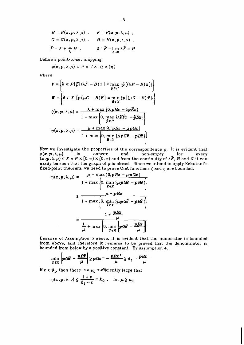
Now we investigate the properties of the correspondence (p. It is evident tha t ( P ( ~ s P I A , ~ ) is convex and non-empty for every ( 2 . p . A,p) E X x P x [0, m) X [ O , =) and from the continuity of @, B and G i t can easily be seen that the graph of (p is closed Since we intend to apply Kakutani's fixed-point theorem, we need to prove that functions [ and q are bounded:

p + rnax IO.pI3k - pp& q ( z , p , X , p ) =

j l p e N - p S j I

- + rnax 0, rnin pGz" - =m Because of Assumption 5 above, it is evident that the numerator is bounded from above, and therefore it remains to be proved that the denominator is bounded from below by a positive constant. By Assumption 4,

If e < dl, then there is a pa sumciently large that

Let us now consider the function #: A + max IO,pBz - hp&j

C ( P , 2 , A , L L ) = # .

A + max 10,pBz - Apfi - pHz ] s f \

1 + max 10. gi;p"thfi + Hz - Bzj I h + max 10,pBz - A p k ]

5 I I

As the boundedness of the numerator is once again obvious, the denominator remains to be investigated:

max [ 0, max 5 E p u l p fi - - ~ ] ] 2 ~ z : f i ( f i - ~ ]

2 1 9 ~ min z jpi+j - A &=&zCE A

Utilizing the fact that 3 > 0 and arguing as above, we can find a constant k and a Ao, such that

t ( z , p , A . p ) 5 k l , when A z A 0

Since X x P x [O,ko] x 10, k l j is compact and the functions 4 and 7 are continu- ous, there exists a constant k such that 0 < # 5 k , and 0 5 r ] 5 k . Therefore the correspondence 9 maps the function X x P x [0, k] x [0, k] into itself, and hence, by the Kakutani theorem, q has a fixed point ( z , p , A,p).

To complete the proof we need to show that, for suitable values of e , a, s, and t , (2 , p , A. & e , a , s, t ) meets the conditions of eqns. (1)-(9).

I. z E w ( z , P , A , ~ )

2. p E V ( z , p , A , p )

3. A = A + max 1 0 . p ~ ~ - hp&j

~AP& -* 1

From 3 we obtain:

1 A p " h - p"Bz j = max jo,p& - A p h j

We shall now prove that p& - A p h = 0. If A = 0, then rnax IO.p& - 0 . phj = 0, tha_t is, p E z = p H = . Now, suppose that A > 0. First, assume that p B z - A p F k < O . Since A > O , we have that maxGEp (hF& -5Bzj < - 0, that is. A p h -P& 5 0, which contradicts the origi- nal assumption. Now, assume that p B z - Ap&> 0. Since A > 0 and p E V, we have that

0 < rnax tAp"& -FEZ ] = A p h - p B z g € P

which is again impossible.

In a similar way we can show from 1 and 4 that

ppGz - p m = 0

Since p E V and z E W,

p"(a -*) ~ p ( h h -B) = 0 = ( p P ~ - p ~ ) z

g (ppG - p B ) Z , whenever @,z") E P x X

From these relations i t trivially follows that

(A& - Bz), & - ei < O+ pi = pi- -

To complete the proof of the theorem we need to investigate whether A'> 0 and F > 0. The case of p = 0 is impossible (since t = p B r 0 from Assumption 5 and 0 < z+t = sz' = 0); consequently p > 0. Since pGr > 0, pBz is also positive. Because ApR + p H z =pbh: if A is zero, i t follows that 0 < p B z = phk s rnax t0,pbh: - p & j, which is impossible since pGz > 0. Q.E.D.

2. ON A SPECIFICATION OF THE MODEL Using the framework of the model described in Section 1, a wide range of

specifications can be developed, within which narrower fields of investigation can be pursued using individual elements of differing degrees of sophistication. This part of the paper, therefore, will emphasize the specific characteristics of the applied model as opposed to the general framework. The points elucidated in this way will be partly economic (or planning) in nature and partly computa- tional (or algorithmic).

2.1. Growth and Profit Factors One of the features of the model discussed is that i t assumes that there are

general growth (A) and profit (b) factors in the economy, which prevail in every sector. However, if we want to speed up growth or seek remedies for particular economic problems it is quite evident that the structural set-up of the economy must be modified.

Ideas on how the growth and profit factors should differ by sectors can be included in the form

where:

I' is a diagonal, whose elements represent how individual sectoral growth factors differ from the economy-wide factor (A),

.k is a diagonal that expresses the differences between sectoral profit factors and the economy-wide factor (p).

2.2. Quasidynamic Properties The production and price variables of the model can trace the process from

period t to period t + 1. If z denotes the activity level in period t , that in period t + 1 will be hrz. Furthermore, we can take the sectoral price levels in period t as unity, and so we can define vector p as the changes in prices for the next period. In this case, the production in "new" prices is given by h < p > rz.

These quasidynamic properties can only be referred to the primal form of the equation, because the dual is only a price-formation rule.

2.3. Alternative Technologies in the Model The general framework of the specification makes it possible to use various

different "technologies" in the model. When the model is used for planning pur- poses the role of different "technologies" can be taken over quite straightfor- wardly by the different plan variants under consideration. Thus in an e z post analysis the role of variants can be successively assigned to the "plan" for the year and to the "fact" that has been realized on the basis of the plan. This approach makes it possible to compare plan and fact and analyze any discrepancies between them.

T h e alternatives can be built into the model in two ways, namely through the matrix coefficients and through the constraints used for production and price ihdices. In the model specification the plan and fact alternatives were used fdr each of the major planning categories studied. Thus the two alterna- tives figure side-by-side and are represented by the following parameter ensem- ble:

material inputs:

A = ( + . A J )

structure and level of consumption:

~ ( b ) E RXzn

where c p , cr E R describe the consumption structure and the d = ( d p , d f ) are parameters controlling the level of consumption;

wage rates:

v = (up ;v , ) E R~~

depreciation rates: d = ( d p ; d f ) E R~~ rn = v + d

outputmatrix:

BO E Rn x2n

2.4. Pricing System In a planned economy different pricing systems can be formed. In the

model speciflcation a simple price-formation rule is built in, namely that the price should cover the cost of raw materials, wages, and the depreciation of the means of production. The profit is proportional to the sum of these three items, but the costs of production in the individual sectors are included in the price with different weights (*) depending on economic and political considera- tions. In order to calculate the economy-wide profit rate, the sectoral price indices are selectively further modified by taxes that burden and subsidies that beneflt the sectors. In this way, through the weight parameters and the taxes and subsidies, a two-step balancing mechanism is built into the model.

2.5. Investments In the model the source of investments is the amount of profit realized by

production z. This amount of profit can be written down as:

The average profit factor (total income divided by total costs) is given by

whence:

E ( p , z ) = (p - l )(pA+ + m+)z

Let us assume that the ratio of investments originating from profit ( g ) and the investment structure ( b ) is exogenously given. Thus the total investment can be written as d z , where

Returning to the dynamic features we note that the investment of a given period can be associated with the production of the same period in a fairly natural way. The general primal equation (I), however, permits a time-lag of one period between protfuction and investment; that is, the production of a given year can be the basis of investment in the following year.

2.6. Constraints and Balances Two remarks are necessary concerning constraints. First, since we are

considering a single output system with alternative technologies we should apply constraints to the output levels (i.e. B O Z ) rather than to the activity lev- els ( 2 ) . Secondly, the relation assumed for export and import price indices in Section 1 (i.e. that the export price index is lower than the import price index and that the domestic price index lies zomewhere in between) has held t rue in practice during the past few years, so that their application as lower and upper bounds, respectively, seems reasonable. Turning to balances, when the foreign trade balance is planned i t is usually not fixed a t zero but i t can be positive or negative according to the aims of economic policy. The same is also t rue of the balance of taxes and subsidies.

2.7. Further Modifications Because of the two alternatives included in the specification t he output

can be obtained as the sum of production activities carried on with individual alternative conditions. The output matrix, therefore, is @ = (I, I). where I is a unit matr ix of order n . This is now the specification of a von Neurnann- Leontief-type model. Mainly for computational reasons, the right-hand side equations of (10) and (11) (i.e. equations ep = ip and tz = sz) are not required. In this way the complementary equations are relaxed.

2.8. Complete Formal Statement of the Model

This formulation of the model can easily be traced back to one similar t o tha t described by eqns. (1)-(1 I), by introducing the following notation:

h the course of the calculations a special type of A-matrix was used, which included not only domestic eupplies of raw materials but also any imports indispensable for production. This latter volume of imports must be equaled by exporte. Therefore s and i represent the surplus valuea above this limit. In eqns. (18) and (19) a1 and ae stand for the planned balances of foreign trade and the budget, respectively.

and for (15):

Differences between the two formulations will remain in the complementary equations and in (14).

2.9. O n the Solution of the Specified Model With a slight modification to Theorem 1, the existence of a solution for the

model system (12)-(19) can also be proved. However, although the applied ver- sion is much simpler, this theorem (being nonconstructive) offers no method for i ts solution. The properties of the specification itself must, therefore, also be investigated.

The overall problem (12)-(19) falls into two parts, since we have omitted the right-hand-side equations of (10) and ( l l ) , i.e. the equations ep = ip and tz = sz. The two subproblems will be formulated as follows:

Aprimal (P) problem: (12), (14), (16), (18); and

A dual (D) problem: (13), (15), (17), (19).

None of the variables of problem (P) are found in problem (D). Making use of Proposition 1 (below), problem (D) can be solved with ease; then with this solu- tion problem (P) can also be solved similarly.

RopoSi t ion 1. I f a > 0, Z'B 2 z - B 2 - 0, and z - B # 0, for an a rb i t r a r y b , t hen p, t , and s are the so lu t ion of

b = p a + t - s

i f and on ly i f

z b - a2 p = max ( 2 - B s z ~ Z + B

Proposi t ion 1A. I f h > 0, p+ 2 p' 2 - 0, and p- # 0, for an arb i t ra ry g , t h e n A, 8 , and i are the so lu t ion of

i f a n d on l y i f

A = min P - I P gP+]

R o o f of A.oposi.tion 1. If p. t , and s are the solution of (20). then

t, =rnaxlO,bj -pail

sj = max 10, paj - b j j

and

z+Bt - z-Bs = z(p)(b - p a )

where I

Finally, for p, t , and s as a solution of (20), it follows that

a2 = z + ~ t -z'B = z(p)(b -pa)

; ? z ( b - p a ) V Z E X

that is,

Conversely, if

zb - a2 ji = rnax

za

then there exists z@) E X , so that

and (23) also holds true. Now we And that = t (fi) and s = s(fi), by (23), and ji, F, and s^, are a solution of (20). Q.E.D. (The proof of Proposition 1A is analo- gous.)

The basic solut ion algorithm is as follows:

Choose p so that p - 6 p g p + and, computing a and b by means of (pA + m) + = a and p ~ O = b , respectively, solve (21). The values of t and s can then be determined using (22) with the optional p.

CQoose z so that z-B S z SZ 'B and solve (21A). where B z - HOZ = g and (A + C(6))T'z - h. The values of e and i can then be easily computed with the optimal A.

From the above i t can be seen that the system (12)-(19) has several solu- tions. The question, therefore, arises as to which X is maximal (and conse- quently which p. is minimal), subject to (12)-(19). Answering this question necessitates the solution of a nonlinear programming problem. An algorithm for this purpose has also been developed (Eels6 et al. 1983). In this algorithm. first p. is minimized subject to the constraints of problem (D), and then in the second step the maximum of A is sought, subject to the constraints of (P). The

following property of (D) can be utilized in its solution: if in (13), (15), and (19) there exists a solution with pO, then one also exists for every p 2 pO, and if p is a minimum the conditions of (17) are also met. Thus, the minimum p and also the other variables associated with p will be determined through the solution of a series of linear equation systems. Similarly, the solution of (P) is based on the property that (12), (14), and (18) can be solved for every A in the interval (-m, Am,,], and if h is a maximum the conditions of (16) are also satisfied.

2.10. Results of Model Calculations In this section we report some of the more characteristic features of model

computations carried out for the year 1979. Three topics will be touched upon, namely the most aggregate figures for growth and profit rates, the alternatives chosen, and some dual-type indicators.

Table 1 shows the most aggregate results of nine computations; these are distinguished on the basis of three criteria:

a. Wage rate in three variants (higher, average, lower);

b. Foreign trade balance in four variants. of which number 1 is the "worst" and number 4 the "best";

c. Extremal values of growth and profit rates (from the solution algo- r i thm it can be seen that the maximum A and the minimum p are of particular importance).

In Table 1 the following points deserve special attention. First, on comparing computation 1 (which is considered to be the basic variant) with computations 2 and 3, it is clear how sensitive the growth rate is to improvements in the foreign trade balance. Second. computations 4-6 show how the growth rate decreases with a 0.05 increase of profit factor. Third, computations 7-9 show that an increase in the wage rate has a positive effect on the growth rate.

TABLE 1 Growth rates and profit factors.

Computation Profit Growth Wage Foreign trade number factor rate (%) levelu balance

7 1.2067 0.00 a 4 8 1.2378 -2.00 1 4 9 1.1750 1.68 h 4 u a. h, and 1 stand for average, higher, and lower levels, respectively.

Table 2 shows how the model chooses between the two alternatives (with the assumptions of computation 1). The table indicates that if the alternatives

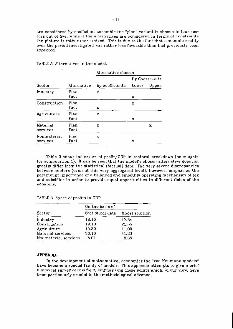
are considered by coefficient ensemble the "plan" variant is chosen in four sec- tors out of five, while if the alternatives are considered in terms of constraints the picture is rather more mixed. This is due to the fact that economic reality over the period investigated was rather less favorable than had previously been expected.

TABLE 2 Alternatives in the model.

Alternative chosen

By Constraints

Sector A1 ternative By coefficients Lower Upper

Industry Plan x Fact x

Construction Plan x Fact x

Agriculture Plan x Fact x

Material Plan x services Fact

Nonmaterial Plan x services Fact

Table 3 shows indicators of profit/GDP in sectoral breakdown (once again for computation 1). It can be seen that the model's chosen alternative does not greatly differ from the statistical (factual) data. The very severe discrepancies between sectors (even at this very aggregated level), however, emphasize the paramount importance of a balanced and smoothly-operating mechanism of tax and subsidies in order to provide equal opportunities in different fields of the economy.

TABLE 3 Share of profits in GDP.

On the basis of

Sector Statistical data Model solution

Industry 18.10 17.84 Construction 19.10 21.55 Agriculture 10.22 11.00 Material services 36.10 41.33 Norimaterial services 5.01 - 5.36

APPENDIX In the development of mathematical economics the "von Neumann models"

have become a special family of models. This appendix attempts to give a brief historical survey of this field, emphasizing those points which, in our view, have been particularly crucial in the methodological advance.

The original von Neumann model may be written as follows:

where z is the production intensity vector, p is the price system, h is the growth factor and p is the interest factor. A denotes the input matrix and B the output matrix. N N denotes non-negativity, P primal. D dual, PC primal com- plementary, and DC dual complementary relations. The primal and the primal- complementary relations represent the conditions of market equilibrium. By (P), supply must be greater than or equal to demand, and by (PC), the prices of free goods must be zero. By (D), none of the sectors can earn extra profit, and by (DC), the activity of unprofitable sectors is not used. These classical equa- tions were first published in 1937 in German and then in 1945 in English. von Neumann proved the existence of an equilibrium in his model by a fixed-point theorem, which later became familiar as Kakutani's fixed-point theorem, von Neumann assumed that the matrices A and B are greater than or equal to zero, and that A + B is strictly positive. The latter assumption was criticized by KemCny e t al. (1956). In their famous article they introduced the well-known KMT (Kem~ny-Morgenstern-Thompson) conditions: the matrix A has nonzero columns and B has nonzero rows. From the economic point of view these assumptions imply first that "there is no output without input" and that all commodities may be produced. Second, they also require that, a t equilibrium, the value of the output pBz should be positive. From this i t follows that the growth factor h and the interest factor p are equal; hence the complementary conditions are superfluous, and the model can be reduced to the much simpler form:

Here PO denotes a positive output value. The existence of an equilibrium in this model can be proved by the Farkas theorem or by other theorems on linear inequalities. It is worth noting that it was only in 1971 that J. Lds, the eminent Polish mathematician, obtained a really simple and elegant proof using only the Farkas theorem. Most textbooks, e.g. Nikaido's Convez S r u c t u r e s and Economic l 'heory, prove the existence theorem by means of the Tucker com- plementarity theorem, which is a fairly &fficult theorem on linear inequalities. Some other textbooks, however, e.g. Gale's Linear Economic Models, prove the consistency of equations (NN), (P), and (D) only, which is intrinsically a much weaker statement.

The drst crucial step in every proof is the determination of the growth fac- tor at the potential equilibrium, which is the maximum possible growth factior.

In this way it is possible to drop out the factor A from the model and thus deal with a simple linear inequality system.

We shall refer to this model below as the symmetrical and linear von Neumann model.

In 1960 Morishima introduced a symmetrical but nonlinear von Neumann- type model with the following equations:

The matrix ~ ( p , A) is a continuous function of the variables p and A, and because of this nonlinearity it is obvious that the equilibrium level of A cannot be determined a p- ior i , and neither can i t be dropped from the model, in con- trast to the symmetrical-linear case. To prove the existence of an equilibrium in this model, it is possible to use one of the Axed-point theorems. Morishima used Eilenberg-Montgomery's theorem, which is unfortunately a difficult one. Morishima's method and ideas are, however, quite straightforward. For every f ixedp and A the linear symmetrical von Neumann model ( ~ ( p , A), B) has some equilibrium solution. The set of these solutions is p(p, A ) . As Nikaido has shown. this set is contractible, and hence the correspondence (p. A) -r p ( p , X ) satisfies the conditions of the Eilenberg-Montgomery theorem. I t should be emphasized that p ( p , A) is not convex, but is only contractible, so that the Kakutani theorem cannot be used.

In 1974 J. Lds defined a linear but asymmetric von Neumann-type model called the three-matrix model:

As i ts name implies, this model consists of three matrices, F, G, and B; B is the usual output niatrix, F is the input matrix, and G is the revenue matrix. In the symmetrical case the revenue and input matrices were equal. But because of the asymmetry in the Lds model, the growth rate and the interest rate are gen- erally different. Therefore the complementary equations are not consequences of the other relations but are independent, and they are frequently the most problematic relations. Lbs has proved the existence theorem by the Kakutani theorem. His proof resembles the original von Neumann proof, and i t can be generalized to the case where the matrices F, G , and B are continuous Punc- tions of the variables z and p. (The proof cannot be extended to the case when the matrices also depend on A and p) The most important step in the proof is the determination of the equilibrium levels of the growth factor A and the interest factor p. As in the symmetrical nonlinear case they are once again not known a p-bri. To illustrate the difficulties in the proof of the existence of an equilibrium in a three-matrix model, we consider the following trivial example:

The matrices F and B satisfy the usual KMT assumption, but the model has no equilibrium solution. The indispensible assumption in the asymmetric von Neumann models is the positivity of G or something similar (e.g. B + G > 0 together with a ( such that F I (G). In the example above, the revenue matrix is not positive so these assumptions are not satisfied. J. Lds has also general- ized his existence theorem to the case when all four matrices are different. One of the most important generalizations of the von Neumann model is the open von Neurnann model of Morgenstern and Thompson:

Several authors have dealt with the Morgenstern-Thompson model (e.g. Mardon 1974, Berezneva and Movshovitch 1975, Moeschlin 1977, Morgenstern and Thompson 1976). In 1976 Ballarini and Moeschlin introduced an asymmetric, linear, open model:

Their proof can also be generalized to the case where F, G, and B are continu- ous functions of z a n d p (see Theorem 1 earlier in this paper).

This paper was o r i g i n a l l y prepared under t h e t i t l e "Modell ing f o r Management" f o r p r e s e n t a t i o n a t a Nater Research Centre (U.K. ) Conference on "River P o l l u t i o n Cont ro l " , Oxford, 9 - 1 1 A s r i l , 1979.

REFERENCES

Ballarini, G. and 0. Moeschlin (1976). An open von Neumann model with con- sumption. In J. Lds e t al. (Eds.), Warsaw Fell S m i n a r s in Mathematical Economics, pp. 1-10.

Bauer, L. (1974). Consumption in von Neumann matrix models. In J. Lds and M. Lds, Mathematical Models in Economics. North-Holland, Amsterdam, pp. 13-27.

Belso, L.. Cs. Cserniitony, and A. Tihanyi (1983). Numerical S l u t i o n of Neumann- type Models. International Simulation and Gaming Association, NVth Open Conference, 13-18 June, Sofia.

Berezneva, T.D. and S.M. Movshovitch (1975). Balanced Growth Equilibrium in Models of the von Neumann Type. Economics and Mathematical Methods (in Russian).

Cheremnikh, Yu.N. (1982). On the Analysis of the Qrobth 73-ujectories of National Economic ModeLs. Nauka. Moscow (in Russian).

Gale. D. (1972). Comment. Econometr ica, 40(2).

Haga, H. and M. Otsuki (1965). On a generalized von Neumann model. h t e r n a - t ional Economic Review, 6: 115-125.

Kemeny, J.G., 0. Morgenstern, and G.L. Thompson (1956). A generalization of the von Neumann model of an expanding economy. Econometrica, 24(2).

Lds, J. (1971). A simple proof of the existence of equilibrium in a von Neumann model and some of i ts consequences. &11. Acad. Polon. Si., Sr , Sci. Math. Astron. e t Rhys., 19:971-979.

Lds, J. (1974). Labour, consumption and wages in von Neumann models. In J. Lds and M.W. Lds (Eds.), Mathematical Models.in Economics. North-Holland, Amsterdam, pp. 67-73.

Lds, J. (1976). Extended von Neumann models and game theory. In J. Lds and M.W. Lds (Eds.), Computing Equilibriu: How and Whv? North-Holland,

Amsterdam, pp. 141-159.

Lds, J. and M.W. Lds (Eds.) (1974). Mathematical Models in Economics. North- Holland, Amsterdam.

Lds, J. and M.W. Lds (1976). Computing Equilibria: How and Why? North- Holland, Amsterdam.

Lds, J., M.W. Lds, and k Wieczorek (Eds.) (1976). Warsaw h 1 1 Seminars in Mathematical Economics.

Makarov, V.L. and A.M. Rubinov (1973). Mathematical Theory of Economic Dyzamics and Equil ibrium. Nauka, Moscow (in Russian).

Mardon, L. (1974). The Morgenstern-Thompson model of an open economy in a closed form. In J. Lds and M.W. Lds (Eds.), Mathematical Models in Econom- ics. North-Holland, Amsterdam, pp. 81-114.

Moeschlin, 0. (1977). A generalization of the open expanding economy model. Econome trica, 45(8).

Morgenstern, 0. and G.L. Thompson (1976). Mathematical lheory of Ezpanding and Contracting Economies. Lexington Books, D.C. Heath and Company, London.

Morishima, M. (1960). Economic expansion and the interest rate in generalized von Neumann models. Econometrica, 28:352-363.

Morishima, M. (1964). Equil ibrium Stability and Growth. Clarendon Press, Oxford.

Morishima, M. (1969). lheory of Economic Growth. Clarendon Press, Oxford.

von Neumann, J. (1937). Uber ein okonomisches Gleichungssystem und eine Verallgemeinerung des Brouwerschen Fixpunktsatzes. Etrgebnkse eines Mathematischen Kolloquiums, No. 8, 1935-1936. Franz-Deuticke, Leipzig and Vienna. [English translation: A model of general economic equilib- rium. Review of Economic Studies. 13 (1945-1946).]