A NONLINEAR FILTER CONTROL CHART FOR DETECTING DYNAMIC CHANGES Nonlinear... · A NONLINEAR FILTER CONTROL CHART FOR DETECTING DYNAMIC CHANGES ... a linear ﬁlter for statistical

Statistica Sinica 20 (2010), 1077-1096

A NONLINEAR FILTER CONTROL CHART

FOR DETECTING DYNAMIC CHANGES

Dong Han1, Fugee Tsung2, Yanting Li1 and Kaibo Wang3

1Shanghai Jiao Tong University,2Hong Kong University of Science and Technology and

3Tsinghua University

Abstract: All conventional control charts can be viewed as charting the output of

a linear filter applied to the process data. In this paper, we present a nonlinear

filter control chart (NFC) in which the control statistic consists of a nonlinear

combination of a data process. We also present a theorem on an estimation of the

average run length for the NFC chart, and we theoretically compare the detection

power of any two such control charts. A criterion is provided for selecting an optimal

NFC chart. In particular, we discuss some special nonlinear filter control charts for

detecting dynamic changes in process mean that can be viewed as extensions of the

conventional CUSUM control charts.

Key words and phrases: Average run length, change point detection, dynamic

changes, statistical process control.

1. Introduction

Since Dr. W. A. Shewhart of the Bell Telephone Labs introduced the statisti-cal process control (SPC) concept and developed the first statistical control chartin the 1920s, many control chart schemes have been proposed. SPC techniquesutilize statistical methods to monitor each phase of the manufacturing processso as to maintain and improve the product quality while decreasing variance.There have been many applications and much development, see Montgomery(2001). This research has focused on efficient, simpler methods for detectingprocess changes accurately and quickly.

In manufacturing, data collected from sensors are contaminated by noisethat is commonly modeled as i.i.d. white noise, drifts, sinusoidal noise, or gen-eral ARIMA time series noise. Conventional control charts can be viewed ascharting the output of a filter applied to process data and to reveal processstatus. A linear filter defines a linear relationship between the purified signaland the contaminated observation. Typically, the output of a filter is a linearfunction of current and perhaps past observations. Some control charts employlinear filters. A Shewhart individual chart uses the original process data, while

1078 DONG HAN, FUGEE TSUNG, YANTING LI AND KAIBO WANG

an Exponentially Weighted Moving Average (EWMA) chart (Roberts (1959))filters process data using a weighted average of past and current observations.Statistics of other popular control charts, such as the Cumulative Sum (CUSUM)chart (Page (1954)), the combined Shewhart-CUSUM chart (Lucas (1982)), theoptimal EWMA (Srivastava and Wu (1993, 1997), Wu (1994)), the generalizedlikelihood ratio (Siegmund (1985), Siegmund and Venkatraman (1995), Apley andShi (1994, 1999)), the adaptive CUSUM (Sparks (2000)), the adaptive EWMA(Capizzi and Masarotto (2003)), and the generalized EWMA (Han and Tsung(2004)) invoke linear combinations of the data process. The ARMA chart (Jiang,Tsui and Woodall (2000)) and the PID chart (Jiang et al. (2002)) use more com-plex forms to combine past and current information for filtering.

Optimal design of a linear filter for statistical process control was proposed byChin and Apley (2007). The underlying ARMA process is identified by applyingan impulse signal; coefficient estimation is achieved and the optimal design iscreated based on the assumed noise type, the charting method, and the desiredin-control average run length (ARL). Simulation shows that this control chartcan outperform existing control charts in some situations.

Although the linear filter-type control chart provides a good way to handlecertain kinds of noise, it has limitations. For instance, the optimal design of alinear filter given by Chin and Apley (2007) depends heavily on the assumedshift magnitude. The magnitude of the shift is, however, rarely pre-specified,but is rather an unknown shift in a possible range, or even a dynamic shift thatchanges over time. Thus, a linear filter may achieve the optimum performance ata single point, but not over the mean shift range of interest. Since linear filtersare designed for detecting certain types of noise, if the actual noise encounteredis different or more complex, the performance of the filter can easily suffer.

To conquer such limitations, we propose extending conventional control chartsthat use linear filters to charts that apply nonlinear filters to the data. We expectthat in presence of more complicated noise, the proposed nonlinear filter controlcharts can prove more capable of handling unknown and dynamic mean shifts,that is, it may respond to mean shifts more quickly. The most popular criterionfor evaluating the responsivity of a control chart is average run length (ARL):the average number of samples (subgroups) taken before an alarming signal isgiven.

In the next section, a nonlinear filter control chart is presented. A theo-rem on an estimation of the average run length, a discussion on the theoreti-cal comparison of any two control charts, and the optimal design of an NFCchart, are given in Section 3. Section 4 gives a comparison of detection per-formance of the nonlinear filter charts and traditional control schemes, by nu-merical simulation. The definition and settings of two adaptive CUSUM charts

A NONLINEAR FILTER CONTROL CHART FOR DETECTING DYNAMIC CHANGES 1079

are shown in Appendix I. The proof of Theorem 1 in Section 3 can be found athttp://www.stat.sinica.edu.tw/statistica as an on-line supplement.

2. A Nonlinear-Filter Control Chart

Here process data are first filtered by a nonlinear filter before being drawnon a chart. We design a nonlinear filter control chart by recalling the well-knownCUSUM chart before extending it.

Let Xi (i = 1, 2, . . .) be the ith observation from an i.i.d. process. Supposeat time τ , called a change point, the mean of Xi abruptly changes from µ0 to µ;Thus, from time τ and on, the mean of Xi undergoes a step mean shift, δ = µ−µ0.We assume µ and τ are unknown, and that µ0 and the standard deviation σ ofthe process {Xi, i ≥ 1} are known. Without loss of generality, µ0 = 0 and σ = 1.

The first time (stopping time) outside the control limit, c > 0, for the one-sided CUSUM chart, T , can be written as

T (δ) = inf{

n : max1≤k≤n

[ n∑i=n−k+1

δ(Xi −δ

2)]≥ c

}, (2.1)

where δ/2 > 0 is the reference value related to the magnitude of the mean shift,δ, see Hawkins and Olwell (1998).

Moustakides (1986) and Ritov (1990) have shown that the performance ofthe one-sided CUSUM control chart with a reference value of δ/2 is optimal ifthe real mean shift is δ. In fact, however, we rarely know the exact magnitude offuture mean shifts. To detect an unknown mean shift quickly, we may considerreplacing δ with {|Xi|} in the CUSUM chart, since {|Xi|} contains real-timeinformation about the magnitude of the mean shift. Thus, we take the stoppingtime of a new control chart to be:

T = inf{

n ≥ 1 : max1≤k≤n

[ n∑i=n−k+1

|Xi|(Xi −|Xi|2

)]≥ c)

}. (2.2)

Here, the control statistic,∑n

i=n−k+1 |Xi|(Xi−|Xi|/2), is a nonlinear combinationof the observed data, {Xi}. Since

|x|(x − |x|2

) =

x2

2 if x ≥ 0

−3x2

2 if x < 0,

we obtain the stopping time of a more general chart,

T (fα) = inf{

n ≥ 1 : max1≤k≤n

[ n∑i=n−k+1

fα(Xi)]≥ c

}, (2.3)

http://www.stat.sinica.edu.tw/statistica


by taking a nonlinear function,

fα(x) =

xα

2 if x ≥ 0

−3|x|α2 if x < 0,

(2.4)

where α > 0. We call T (fα) and fα(·), respectively, the stopping times of anonlinear filter control chart (NFC) and a nonlinear filter function.

Generally, the nonlinear filter is not restricted to the form of (2.4). It cantake any form. When f is a linear function, we call T (f) the stopping time of alinear filter control chart (LFC).

If a negative mean shift is of interest, the stopping time of a general NFCchart can be written as

T (fα) = inf{

n ≥ 1 : min1≤k≤n

[ n∑i=n−k+1

fα(Xi)]≤ −c

}, (2.5)

where fα(x) is

fα(x) =

3xα

2 if x ≥ 0

− |x|α2 if x < 0.

(2.6)

Thus, a two-sided NFC control scheme can be readily constructed.Han and Tsung (2006) proposed a reference-free Cuscore (RFCuscore) chart

that is also capable of tracing and detecting dynamic mean changes quickly with-out knowing the reference pattern or having prior knowledge of the mean shiftmagnitude. The RFCuscore chart is a special case of the nonlinear filter controlchart with α = 2.

3. Theoretical Analysis

For convenience of discussion, we use the standard quality control terminol-ogy. Let P (·) and E(·) denote the probability and expectation functions whenthere is no change in the mean, µ = µ0 = 0; let Pµ(·) and Eµ(·) be the probabilityfunction and expectation function when the change point is at τ = 1, and the truemean shift value is µ 6= 0. The two most frequently used operating characteristicsof statistical control charts are in-control average run length ARL0(T ) = E(T )and out-of-control average run length ARLµ(T ) = Eµ(T ).

For comparison, all candidate charts share the same ARL0 which correspondsto the same level of type I error rate. The chart with the smallest out-of-controlARLµ at the desired mean shift magnitude has the highest power to detect thepre-specified shift.


In this section, we first present a theorem on the estimation of the ARL for ageneral control chart, including NFC and LFC, with a large control limit. Thenwe discuss how to compare the detection performances of any two control charts.

3.1. Approximation, estimation, and comparison of ARL’s

Let Y1, Y2, . . . be i.i.d. observations of a random variable Y , and let F andE be its cumulative distribution function and expectation function. Suppose F

satisfies the following.(I) The moment-generating function h(θ) = E(eθY ) < ∞ for some θ > 0.(II) For x > E(Y ) there is a θ(x) ∈ (0, θ1) such that x = h′(θ(x))/h(θ(x)),

where θ1 = sup{θ : h(θ) < ∞}.Let E(Y ) < 0. Since h′(0) = E(Y ) < 0, h′(θ)/h(θ) is strictly increasing

(see Durrett (1991, p.60)) and log h(θ) → +∞ as θ → θ1, it follows that thereexists at most one θ∗ ∈ (θ(0), θ1) such that h(θ∗) = 1 or log h(θ∗) = 0, whereθ(0) > 0 satisfies 0 = h′(θ(0))/h(θ(0)). That is, h(θ) attains its minimum valueat θ(0) > 0. We can call θ∗ an exponential rate of Y . The meaning of θ∗ isgiven in Theorem 1.

Now we define the stopping time of a control chart as

T = inf{

n : max1≤k≤n

[ n∑i=n−k+1

Yi

]≥ c

}, (3.1)

where c > 0 is the control limit.

Theorem 1. Suppose the conditions (I) and (II) hold. If E(Yi) < 0, then

E(T ) ∼ D(c)ecθ∗ (3.2)

for large c, where θ∗ > 0 is the exponential rate satisfying h(θ∗) = 1, 1/bc ≤D(c) ≤ c/u, u = h′(θ∗) > 0 and b is a positive constant. If E(Yi) > 0, then forlarge c,

E(T ) ∼ c

E(Yi). (3.3)

Here we do not consider the case that E(Yi) = 0 since it is then difficult toestimate the ARL. The proof of Theorem 1 is in Section 3. The on-line sup-plement is at www.stat.sinica.edu.tw. Table 3.1 shows the out-of-control ARLsof NFC charts having α = 1.0 and α = 2.0 in the presence of mean shifts ofmagnitude around θ∗. The results were obtained via Monte Carlo simulation.The values of θ∗ of the two control charts are highlighted in boldface. We cansee that, although the formulas for E(T ) have different forms around θ∗, theout-of-control ARL evolves quite smoothly there.


Table 3.1. Out-of-control ARLs of two NFC charts with α = 1.0 and α = 2.0around θ∗, in-control ARL =700.

α = 1.0, c = 5.148 α = 2.0, c = 10.295δ ARL δ ARL

0.40000 59.8060 0.30000 94.85900.43600 50.2066 0.34300 74.44900.43610 50.1686 0.34310 74.16730.43620 50.1354 0.34320 74.15560.43625 50.0580 0.34330 74.05240.43630 50.0572 0.34340 74.05190.43635 50.0454 0.34350 73.97620.43640 50.0249 0.34355 73.95760.43650 50.0119 0.34360 73.95440.43660 49.9835 0.34365 73.93630.43670 49.9804 0.34370 73.92770.43680 49.9057 0.34380 73.78400.43690 49.8995 0.34390 73.66120.45000 47.0550 0.35000 71.22000.50000 37.9390 0.40000 56.3860

Remark 1. Large c means that the term o(1) in E(T ) = (c/E(Yi))(1 + o(1)) ofTheorem 1 is negligible. For example, if c ≥ 10, then |o(1)| < 1/c ≤ 1/10 = 0.1for the CUSUM chart with δ = 1 and Yi ∼ N(1, 1). As can be seen, the resultsof Theorem 1 can be used for many control charts in detecting the observedprocess that is not necessarily normal. If {Yi} is normal and E(Y ) < 0, then theexponential rate is 2|E(Yi)|/Var (Yi), which can be considered as signal-to-noiseratio. In fact, we write

h(θ) = E(eθY ) = exp{θVar (Y )[θVar (Y ) + 2E(Yi)]

2Var (Y )

}. (3.4)

Thus h(θ∗) = 1 when θ∗ = −2E(Yi)/Var (Yi) = 2|E(Yi)|/Var (Yi).

Theorem 1 can be considered as a generalization of Basseville and Nikiforov(1993, p.162), since Y = log[pθ(X)/pθ0(X)] where pθ(·) and pθ0(·) are two distri-bution functions or two density functions. As an application of Theorem 1, wediscuss how to compare the detection performance of two control charts.

Let Xi, i = 1, 2, . . . be an i.i.d. process with mean Eµ(Xi) = µ ≥ 0. Wesay that there is no mean shift if µ = 0. For any two linear or nonlinear filterfunctions, fj(·), j = 1, 2, we can get two control charts with stopping timesT (fj), j = 1, 2. Let Fj(x) be the distribution function of fj(Xi), j = 1, 2, andlet Ej(µ) = Eµ(fj(Xi)), j = 1, 2. Assume that conditions (I) and (II) hold forFj(x), j = 1, 2, and that Ej(µ), j = 1, 2 are strictly increasing functions on µ ≥ 0


with Ej(0) < 0. Thus, there exist two positive numbers, µ∗1 and µ∗

2, such thatEj(µ∗

j ) = 0, j = 1, 2. For a given µ < µ∗j , let θ∗j (µ) be the exponential rate of

Fj(x) for j = 1, 2.Suppose E0(T (f1)) = E0(T (f2)) = ARL0. It follows from (3.2) of Theorem 1

that D1(c1)ec1θ∗1(0) ∼ D2(c2)ec2θ∗2(0) for large c1 and c2, where c1 and c2 are controllimits, respectively, for T (f1) and T (f2). Thus, c1θ

∗1(0) = c2θ

∗2(0)(1 + o(1)) for

large c1 and c2.Let the mean shift be µ < min{µ∗

1, µ∗2}. By (3.2) of Theorem 1, we have

ARLµ(T (f1)) = Eµ(T (f1)) = (1 + o(1))D1(c1) exp{c1θ∗1(µ)}

= (1 + o(1))D1(c1) exp{

c2θ∗2(0)θ∗1(µ)

θ∗1(0)(1 + o(1))

},

ARLµ(T (f2)) == Eµ(T (f2))(1 + o(1))D2(c2) exp{c2θ∗2(µ)}.

From this, we see that ARLµ(T (f1)) > ARLµ(T (f2)) for large c1 and c2 if andonly if

θ∗1(µ)θ∗1(0)

>θ∗2(µ)θ∗2(0)

. (3.5)

Similarly, for µ > max{µ∗1, µ

∗2}, we get from (3.3) of Theorem 1 that ARLµ(T (f1)) >

ARLµ(T (f2)) for large c1 and c2 if and only if

1θ∗1(0)E1(µ)

>1

θ∗2(0)E2(µ). (3.6)

Suppose µ∗1 < µ∗

2. Then ARLµ(T (f1)) < ARLµ(T (f2)) for µ∗1 < µ < µ∗

2 andlarge c1 and c2. In fact, by Theorem 1, we have

ARLµ(T (f1)) = (1 + o(1))c1

E1(µ)= (1 + o(1))

c2θ∗2(0)

θ∗1(0)E1(µ),

since E1(µ) = Eµ(f1(Xi)) > 0 for µ > µ∗1, and

ARLµ(T (f2)) = (1 + o(1))D2(c2) exp{c2θ∗2(µ)}

for µ < µ∗2. Thus, ARLµ(T (f1)) < ARLµ(T (f2)) for large c2. Similarly, if

µ∗1 > µ∗

2, ARLµ(T (f1)) > ARLµ(T (f2)) holds for µ∗1 > µ > µ∗

2 and large c1 andc2.

These comparisons are applied to the specific NFC examples that are derivedfrom conventional CUSUM charts in the next subsection.


3.2. Examples

Let {Xi, i ≥ 1} be i.i.d. N(µ, 1), µ ≥ 0. Denote the expectation and varianceof gδ(X1), f1(X1) and f2(X1), respectively, by E0(µ), V0(µ), E1(µ), V1(µ), andE2(µ), V2(µ), where gδ(x) = δ(x−δ/2), and fi(·), i = 1, 2, are the functions fα(·)with α = 1, 2 defined in (2.4). Then

E0(µ) = E(gδ(X1)) = δ(µ − δ

2), V0(µ) = Var (gδ(X1)) = δ2,

E1(µ) = µ[32− Φ(µ)] − ϕ(µ),

V1(µ) =94

+ µ2Φ(µ)[1 − Φ(µ)] + ϕ(µ)(µ − ϕ(µ)) − 2Φ(µ)(1 + µϕ(µ)),

E2(µ) = 2µϕ(µ) + (µ2 + 1)[2Φ(µ) − 32],

V2(µ) = 4Φ(µ)(µ2 + 1)2[1 − Φ(µ)] + µ2(4µϕ(µ) + 9) + 4Φ(µ) +92

−4(µϕ(µ) + 1)(µϕ(µ) + 2Φ(µ)(µ2 + 1)),

where Φ(·) and ϕ(·) are the standard normal distribution and density func-tions. It can be shown that Ej(µ), j = 0, 1, 2, are all strictly monotonicallyincreasing functions on µ ≥ 0, with E0(0) = −δ/2, E0(δ/2) = 0, E1(0) =−1/

√2π,E1(0.4363) = 0, and E2(0) = −1/2, E2(0.3436) = 0. Denote the

moment-generating functions and the exponential rates of gδ(Xi) and fj(Xi), j =1, 2, respectively, by h0(θ) and θ∗0(µ), and hj(θ) and θ∗j (µ), j = 1, 2. We then get

h0(θ) = E(eθgδ(X1)) = exp{θδ2(θδ2 + 2δ(µ − δ/2))

2δ2

},

h1(θ) = E(eθf1(X1)) = exp{4µθ + θ2

8

}Φ(µ +

θ

2),

+exp{12µθ + 9θ2

8

}[1 − Φ(µ + 3

θ

2)],

h2(θ) = E(eθf2(X1)) =1√

1 − θexp

{ θµ2

2(1 − θ)

}Φ(

µ√1 − θ

)

+1√

3θ + 1exp

{ −3θµ2

2(3θ + 1)

}[1 − Φ(

µ√3θ + 1

)].

Obviously, h(θ∗0(µ)) = 1 for θ∗0(µ) = (δ−2µ)/δ = |2E(gδ(Xi)|/Var (gδ(Xi)) when0 ≤ µ ≤ δ/2. It is rare for the exponential rate θ∗j (µ), j = 1, 2, to have a closedform, but θ∗j (µ), j = 1, 2, strictly monotonically decrease on 0 ≤ µ ≤ 0.4363and 0 ≤ µ ≤ 0.3436, respectively, with θ∗1(0) = 1.04, θ∗1(0.4363) = 0, θ∗2(0) =0.449 and θ∗2(0.3436) = 0. Note that E1(0) = −1/

√2π, V1(0) = 5/4 − 1/2π,


E2(0) = −1/2, V2(0) = 7/2, and therefore θ∗1(0) = 1.04 6= 2|E1(0)|/V1(0) andθ∗2(0) = 0.449 6= 2|E2(0)|/V2(0).

Using Theorem 1, we can get the approximate ARL’s for the CUSUM chartwith stopping time T (gδ), and the NFC charts with stopping times, T (fj), j =1, 2. Thus

ARLµ(T (gδ)) ∼ D0(c)ec(δ−2µ)/δ, ARLµ(T (gδ)) ∼c

δ(µ − δ/2),

respectively, for 0 ≤ µ < δ/2 and µ > δ/2, and

ARLµ(T (fj)) ∼ Dj(c)ecθ∗j (µ), ARLµ(T (fj)) ∼c

Ej(µ),

respectively, for 0 ≤ µ < µ∗j and µ > µ∗

j , j = 1, 2, where µ∗1 = 0.4363 and

µ∗2 = 0.3436.

Note that the ARLs for the CUSUM chart, ARLµ(T (gδ)), are consistentwith the known results when the control limit is large (see Srivastava and Wu(1997)).

Suppose that the control limits of T (f1), T (f2), and T (gδ)) have a largecommon in-control ARL0. By checking (3.5) and (3.6) for the three charts, wecan make comparisons.

Remark 2. (1) ARLµ(T (f1)) <ARLµ(T (f2)) for 0.6597 < µ < 1.7162, andARLµ (T (f1)) > ARLµ (T (f2)) for 0 < µ < 0.6597 and µ > 1.7162.

(2) For δ = 1, ARLµ(T (gδ) > ARLµ(T (f1)) for 0 < µ < 0.7645, ARLµ(gδ) <

ARLµ(T (f1)) for µ > 0.7645, ARLµ(T (gδ)) > ARLµ(T (f2) for 0 < µ < 0.7164and µ > 3.5437, and ARLµ(T (gδ)) < ARLµ(T (f2)) for 0.7164 < µ < 3.5437.

The one-sided CUSUM control chart with a reference value of δ/2 is optimal:ARLµ(T (gδ) is the smallest if the real mean shift is δ. It follows from Remark 2 (2)that both ARLµ(T (f1)) and ARLµ(T (f1)) are shorter than ARLµ(T (gδ) whenthe real mean shift µ satisfies 0 < µ < 0.7645 < δ = 1 and µ > 3.5437 > δ = 1,respectively. The optimality of the CUSUM control chart thus depends on thechoice of reference value δ/2.

Although these theoretical comparisons are based on the condition that thecontrol limits, and therefore the common ARL0, are large, the simulation resultsin the next section produce results consistent with Remark 2.

Remark 3. Take the nonlinear filter fα defined in (2.4) and let {Yi(α) =fα(Xi), i ≥ 1}, where {Xi, i ≥ 1} is i.i.d. normal. We have E(eθY1(α)) = +∞ forα > 2 and any θ > 0. That is, condition (I) and therefore result (3.2) in Theorem1 do not hold for {Yi(α), i ≥ 1} when α > 2. Thus, (3.5) and (3.6) cannot be


used for the case of α > 2. However, the results in the next section show thatthe two nonlinear filter control charts with stopping times T (fα) for α = 2.5 andα = 3, respectively, have good detection performance in the presence of dynamicmean shifts.

3.3. Design of an optimal NFC chart

The nonlinear filter control chart provides great flexibility in functionalforms, although the optimal design of such a control chart is challenging. Theo-retically, any function could be a candidate for the optimal choice. Here, we onlyconsider filter functions in

D0 = {f : Eµ(f(Xi)) satisfies conditions (I) and (II) with E0(f(Xi)) < 0}.

If a NFC chart, defined at (2.3) with f∗(·) in D0, has the best performance indetecting the unknown mean change in the range (0, R), where 0 < R ≤ ∞, wecall it the optimal filter function. Based on Section 3.1 and the inequalities (3.5)and (3.6), we can conclude that the exponential rate and the expectation of theoptimal filter function, f∗(·) satisfy

a

∫ µf∗∧R

0

θ∗f∗(µ)θ∗f∗(0)

dµ + b

∫ R

(µf∗+ε)∧R

1θ∗f∗(0)Eµ(f∗(X1))

dµ

= minf∈D0

{a

∫ µf∧R

0

θ∗f (µ)θ∗f (0)

dµ + b

∫ R

(µf+ε)∧R

1θ∗f (0)Eµ(f(X1))

dµ

}, (3.7)

where a, b, are two given positive constants with a + b = 1, ε is a small positivenumber, µf satisfies Eµf

(f(X1)) = 0, Eµ(f(X1)) < 0 for 0 ≤ µ < µf , andEµ(f(X1)) > 0 for µ > µf . Here, a and b represent, respectively, the weightof “small mean change, 0 < µ < µf” and “large mean change, µ > µf”. Theoptimal filter function f∗(·) defined in (3.7) usually depends on a, b, ε and R.

While (3.7) provides a unified criterion for selecting an optimal control chartfor either NFC or LFC, it is not easy to obtain the optimal NFC chart since thefunctions θ∗f (µ)/θ∗f (0) and θ∗f (0)Eµ(f(Xi)) usually have no closed form. If the setD0 could be reduced, obtaining the optimal NFC chart becomes possible. Forexample, let {Xi, i ≥ 1} be i.i.d. N(µ, 1), where µ ≥ 0. Let

D0 = D0(R, ε) = {fδ : fδ(x) = δ(x − δ/2), |x| < ∞, 0 < δ < 2(R − ε)},

where R > 0, ε > 0. Obviously, for any fixed δ > 0, fδ(X1) satisfies conditions (I)and (II). Since θ∗fδ

(µ) = (δ−2µ)/δ for 0 ≤ µ < δ/2, µfδ= δ/2 and Eµ(fδ(X1)) =

δ(µ − δ/2) for µ > δ/2, it follows that

a

∫ µf∧R

0

θ∗f (µ)

θ∗f (0)dµ + b

∫ R

(µf+ε)∧R

1θ∗f (0)Eµ(f(X1))

dµ


= a

∫ δ/2

0(1 − 2µ

δ)dµ + b

∫ R

(δ/2+ε)∧R

1δ(µ − δ/2)

dµ

=aδ

4+

b

δ[ln(R − δ

2) − ln ε] , H(δ).

We further have H ′(0) = −∞,H ′(2(R − ε)) = a/4 − b/(4ε(R − ε)), and

H ′′(δ) =2b

δ3[ln(R − δ

2) − ln ε] +

b(4R − δ)δ2(2R − δ)2

> 0

for 0 < δ < 2(R − ε). If aε(R − ε) ≤ b, then H(2(R − ε)) = inf0≤δ≤2(R−ε) H(δ).Thus, the optimal filter function in D0(R, ε) is f∗(x) = (2R − ε)(x − R − ε). Ifaε(R− ε) > b, then H(δ∗) = inf0≤δ≤2(R−ε) H(δ), and therefore, the optimal filterfunction is f∗(x) = δ∗(x − δ∗/2), where δ∗ is the unique solution to

H ′(δ) =a

4− b

δ2[ln(R − δ

2) − ln ε] − b

δ(2R − δ)= 0

for 0 ≤ δ ≤ 2(R − ε).

4. Simulation and Comparison

In this section, we further demonstrate that the nonlinear filter control chartsare superior at detecting dynamic mean shifts.

We chose nine control charts for comparison, a two-sided CUSUM chart withδ = 1, six two-sided nonlinear filter charts with α = 1.0, 1.5, 1.8, 2.0, 2.5, and 3.0,denoted by NFCα, and two adaptive CUSUM charts proposed by Sparks (2000)because they are specifically designed for detecting shifts within a range. Ac-cording to the Sparks (2000)’s recommendation, we build two adaptive CUSUMcharts, ACUSUM1 and ACUSUM2, for comparison purposes. The definitionsand settings of the two adaptive CUSUM charts are shown in Appendix I.

Observations, Xi, i ≥ 1, were i.i.d. normal N(µ, 1). The possible mean shiftvalues were µ = 0.05, 0.1, . . . , 6. As for the dynamic mean shifts, we assumedthat Xi, i ≥ 1, were mutually independent and Xk ∼ N(µpk, 1), with four typesof dynamic mean shifts {µpk} studied, respectively, in Figures 4.2−4.4. Figure4.1 compares simulation results for step shifts in process mean, while Figures4.2−4.5 contain results for four types of dynamic mean shifts. For dynamicmean shifts, the definition of the first time (stopping time) outside the controllimit was the same as (2.3). Note that the results of Theorem 1 are not truefor the stopping time of the dynamic mean shift, since Yk = fα(Xk), k ≥ 1, haddifferent distributions, where Xk ∼ N(µpk, 1) and fα is defined in (2.4).

The numerical ARLs were obtained from 1,000,000 Monte Carlo simulations.Although ARL is a popular criterion, it is deficient in evaluating the charting


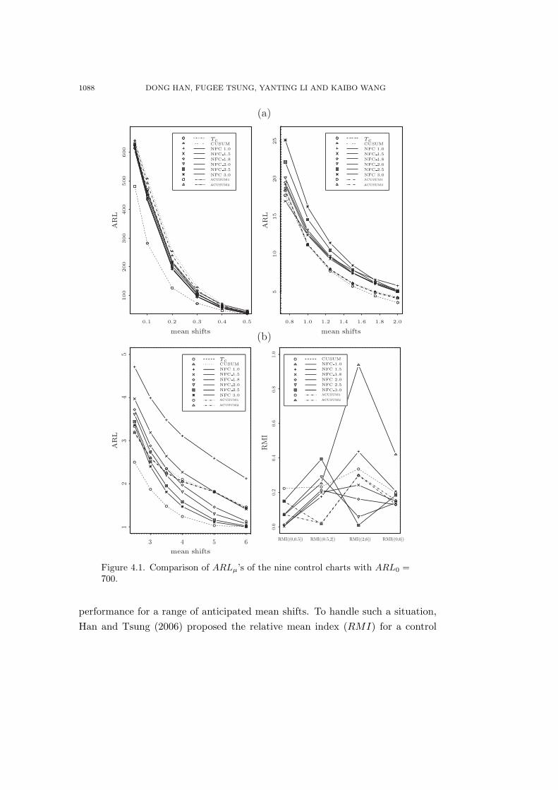
Figure 4.1. Comparison of ARLµ’s of the nine control charts with ARL0 =700.

performance for a range of anticipated mean shifts. To handle such a situation,Han and Tsung (2006) proposed the relative mean index (RMI) for a control


Figure 4.2. Comparison of ARLs of the nine control charts with ARL0 =700, pk = 3/4 + 1/4(1/2)k−1.

chart as

RMI(a, b] =1n

n∑i=1

[ARLµi(T ) − ARL∗

µi

ARL∗µi

], (4.1)


Figure 4.3. Comparison of ARLs of the nine control charts with ARL0 =700, pk = 5/4 − 1/4(1/2)k−1.

where µi and 1 ≤ i ≤ n are the mean shifts in the anticipated range (a, b](0 < a < b) within which the control chart performance is evaluated, ARLµi(T )


Figure 4.4. Comparison of ARLs of the nine control charts with ARL0 =700, pk = 1 + cos(kπ/4).

is the ARL of a control chart when the real mean shift is µi. Here ARL∗µi

denotesthe smallest value of ARL of all control charts in comparison when the mean shift,


Figure 4.5. Comparison of ARLs of the nine control charts with ARL0 =700, pk = 1 + (−1)k/2.

µi, occurs. Obviously, the smaller RMI(T ), the better the control chart is at


detecting mean shifts on the whole. Rather than using ARL at a specific shiftmagnitude as a criterion, the proposed RMI can take all the possible mean shiftswithin a range into consideration.

Figures 4.1−4.5 give the detailed numerical results of the out-of-control av-erage run length. Here, all control charts were two-sided, and their commonin-control ARL0 was fixed at 700. RMI((0, 0.5]), RMI((0.5, 2]), RMI((2, 6]),and RMI((0, 6]) are the relative mean index (RMI) of the small, medium andlarge mean shifts, respectively. The smallest RMI values for a specific meanshift are highlighted in boldface.

We first compare the results in Remark 2 with the Monte Carlo simulationresults of the NFC charts.

Remark 4. (1). In Figure 4.1, for step shifts in the process mean, we haveARLµ(T (f1)) < ARLµ(T (f2)) for 0.55 < µ < 1.36, and ARLµ(T (f1)) > ARLµ

(T (f2)) for 0 < µ < 0.55 and µ > 1.36.

(2). In the presence of step changes in the process mean, for δ = 1, α = 1, andα = 2, we have ARLµ(TC(1)) > ARLµ(T (f1)) for 0 < µ < 0.70, ARLµ(TC(1)) <

ARLµ(T (f1)) for µ > 0.70, ARLµ(TC(1)) > ARLµ(T (f2)) for 0 < µ < 0.64 andµ > 3.02, and ARLµ(TC(1)) < ARLµ(T (f2)) for 0.64 < µ < 3.02.

Compared with Remark 2, we conclude that the theoretical results for largecontrol limits are basically consistent with the simulation results for ARL0 = 700.

For step mean shifts, Bagshaw and Johnson (1975) showed that the optimalconventional CUSUM chart for detecting a mean shift µ is the CUSUM chart withδ = µ/2. Therefore, in Figure 4.1, besides the ARLs of the nine control charts,the ARLs of the conventional two-sided CUSUM control chart with stoppingtime TC , with a reference value of µi/2 when the real mean shift is µi, are alsoshown. Obviously, the NFC charts with α = 1.8 and α = 3, respectively, performthe best in detecting small and large mean shifts. The adaptive CUSUM chart,ACUSUM2, has higher capability in detecting medium mean shifts. However,with regard to RMI((0, 6]), the NFC chart with α = 2.0 has better overallperformance than the CUSUM chart and the adaptive CUSUM charts.

In Figures 4.2−4.5, we show the performance of six NFC charts, one conven-tional CUSUM chart, and two adaptive CUSUM charts in the presence of fourtypes of dynamic changes. Figures 4.2 and 4.3 show the effects of two types ofdamping mean shifts, (3/4 + 1/4(1/2)k−1)µi and (5/4 − 1/4(1/2)k−1)µi. Obvi-ously, these mean shifts increase and decrease, and finally stabilize at µi/4 and5µi/4. In Figure 4.4, a cyclic mean shift, (1+ cos(kπ/4))µi is considered. Figure4.5 shows how the control charts can detect “zigzag” mean shifts.

In Figure 4.2, the NFC chart with α = 1.8 and the NFC chart with α = 3.0,respectively, had the best performances in detecting small and large mean shifts.


With regard to medium mean shifts, the conventional CUSUM chart beats allother charts with its smallest RMI values. However, judging from RMI((0, 6]),the NFC chart with α = 2.0 enjoyed the best overall performance. Similarconclusions can be drawn from Figure 4.3. The NFC charts still outperformedthe other two types of control charts in detecting small, large and overall meanshifts.

In Figure 4.4, the advantage of the NFC control charts still remains. Forsmall and medium mean shifts, nearly all of the NFC charts performed betterthan the competing control charts. The NFC chart with α = 1.8 had the highestcapability in detecting small and medium mean shifts. As to large mean shifts,the conventional CUSUM chart had the best performance. However, with respectto the overall performance, the NFC chart with α = 2.5 was the best. Therefore,in detecting cyclic mean shifts, NFC charts appear preferable to the conventionalCUSUM chart and the adaptive CUSUM charts.

With regard to “zigzag” mean shifts, Figure 4.5 shows that NFC charts candetect small and large mean shifts. The NFC chart with α = 3.0 was the bestfor detecting large mean shifts, while the NFC chart with α = 1.8 performedthe best in the presence of small mean shifts. Although the conventional controlchart was most suitable for detecting medium mean shifts, the NFC chart withα = 2.0 was the best for detecting a mean shift over the range (0, 6].

In summary, we found NFC charts more capable of detecting constant ordynamic shifts in process mean. In particular, for step mean changes, the NFCchart with α = 2.0 had better overall detection capability than either CUSUMor adaptive CUSUM charts. For damping mean shifts, we recommend using theNFC control chart with α = 2.0. For cyclic mean shifts, (1 + cos(kπ/4))µi, twoNFC control charts with α = 1.8 and α = 2.5 were better choices.

Acknowledgement

We thank the Editors and the referees for their valuable comments and sug-gestions that have improved both the content and presentation of this work.This research was supported by RGC Competitive Earmarked Research Grants620606 and 620707.

Appendix I.

The control statistics of the two-sided adaptive CUSUM chart proposed bySparks (2000) are

δ̂Ut = max(αxt−1 + (1 − α)δ̂U

t−1, δUmin),

ZUt = max

(0, ZU

t−1 +[xt − δ̂U

t /2]h(δ̂U

t )

),


δ̂Lt = min(αxt−1 + (1 − α)δ̂L

t−1, δLmax),

ZLt = min

(0, ZL

t−1 +[xt − δ̂L

t /2]

h(−δ̂Lt )

),

where xt is the original observation of the process, δ̂Lt and δ̂U

t are the one-step-ahead forecast of the mean shift at time t, δL

max and δUmin, respectively, denote the

smallest downside and upside mean shifts that are of interest, h(δ) is the controllimit of the conventional CUSUM chart when its reference value is k = δ/2, andthe in-control ARL is a pre-specified value, here it is 700. ZL

t and ZUt are the

plotted statistics. The control chart signals whenever ZLt < −hz or ZL

U > hz.The value of hz is chosen to achieve a specified in-control ARL of the adaptiveCUSUM chart.

Sparks (2000) recommended using α = 0.1, δLmax = −0.5, δU

min = 0.5, δ̂L1 =

−1, δ̂U1 = 1 for detecting smaller shifts, and α = 0.1, δL

max = −0.75, δUmin =

0.75, δ̂L1 = −1, δ̂U

1 = 1 for detecting larger shifts. We denote them, respectively,as ACUSUM1 and ACUSUM2.

References

Apley, D. W. and Shi, J. (1994). A statistical process control method for autocorrelated data

using a GLRT. In Proceeding of the International Symposiumon Manufacturing Science

and Technology for 21st Century, 165-170. Tsinghua Press, Beijing.

Apley, D. W. and Shi, J. (1999). The GLRT for statistical process control of autocorrelated

processes. IIE Trans. 31, 1123-1134.

Bagshaw, M. and Johnson, R. A. (1975). The influence of reference values and estimated variance

on the ARL of CUSUM tests. J. Roy. Statist. Soc. Ser. B 37, 413-420.

Basseville, B. and Nikiforov, I. V. (1993). Detection of Abrupt Changes: Theory and Application.

Prentice-Hall, Englewood Cliffs, NJ.

Capizzi, G. and Masarotto, G. (2003). An adaptive exponentially weighted moving average

control chart. Technometrics 45, 199-207.

Chin, C. and Apley, D. W. (2007). An optimal filter design approach to statistical process

control. J. Quality Tech. 39, 93-117.

Durrett, R. (1991). Probability Theory and Examples. Wadsworth, California.

Han, D. and Tsung, F. (2004). A generalized EWMA control chart and its comparison with the

optimal EWMA, CUSUM and GLR schemes. Ann. Statist. 32, 316-339.

Han, D. and Tsung, F. (2006). A reference-Free Cuscore chart for dynamic mean change de-

tection and a unified framework for charting performance comparison. J. Amer. Statist.

Assoc. 101, 368-386.

Hawkins, D. M. and Olwell, D. H. (1998). Cumulative Sum Charts and Charting for Quality

Improvement. Springer. New York.

Jiang, W., Tsui, K. L. and Woodall, W. H. (2000). A new SPC monitoring method: the ARMA

chart. Technometrics 42, 399-410.


Jiang, W., Wu, H., Tsung, F., Nair, V. and Tsui, K. L. (2002). Proportional integral derivative

charts for process monitoring. Technometrics 44, 205-214.

Lucas, J. M. (1982). Combined Shewhart-CUSUM quality control scheme. J. Quality Tech. 14,

51-59.

Montgomery, D. C. (2001). Introduction to Statistical Quality Control. Wiley, New York.

Moustakides, G. V. (1986). Optimal stopping times for detecting changes in distribution. Ann.

Statist. 14, 1379-1387.

Page, E. S. (1954). Continuous inspection schemes. Biometrika 41, 100-115.

Ritov, Y. (1990). Decision theoretic optimality of the cusum procedure. Ann. Statist. 18, 1464-

1469.

Roberts, S. W. (1959). Control charts based on geometric moving averages. Technometrics 1,

239-250.

Siegmund, D. (1985). Sequential Analysis: Tests and Confidence Intervals. Springer-Verlag, New

York.

Siegmund, D. and Venkatraman, E. S. (1995). Using the generalized likelihood ratio statistic

for sequential detection of a change-point. Ann. Statist. 23, 255-271.

Sparks, R. S. (2000). CUSUM charts for signalling varying location shifts. J. Quality Tech. 32,

157-171.

Srivastava, M. S. and Wu, Y. H. (1993). Comparison of EWMA, CUSUM and Shiryayev-

Roberts procedures for detecting a shift in the mean. Ann. Statist. 21, 645-670.

Srivastava, M. S. and Wu, Y. H. (1997). Evaluation of optimum weights and average run

lengths in EWMA control schemes. Comm. Statist. Theory Methods 26, 1253-1267.

Wu, Y. H. (1994). Design of control charts for detecting the change. In Change-point Problems

(Edited by E. Carlstein, H. G. Muller and D. Siegmund), 330-345. IMS, Hayward, CA.

Department of Mathematics, Shanghai Jiao Tong University, Shanghai, China.

E-mail: [email protected]

Department of Industrial Engineering and Logistics Management, Hong Kong University of

Science and Technology, Kowloon, Hong Kong.


Department of Industrial Engineering and Management, School of Mechanical Engineering,

Shanghai Jiao Tong University, Shanghai, China.


Department of Industrial Engineering, Tsinghua University, Beijing, China.


(Received March 2008; accepted April 2009)

Documents

A NONLINEAR FILTER CONTROL CHART FOR DETECTING DYNAMIC CHANGES Nonlinear... · A NONLINEAR FILTER CONTROL CHART FOR DETECTING DYNAMIC CHANGES ... a linear ﬁlter for statistical