A non-supersymmetric model withunification of electro-weak and strong

interactions

R. Frezzottia) M. Garofalob) G.C. Rossia)c)

a) Dipartimento di Fisica, Universita di Roma “Tor Vergata”

INFN, Sezione di Roma 2

Via della Ricerca Scientifica - 00133 Roma, Italy

b) Higgs Centre for Theoretical Physics, School of Physics and Astronomy,

The University of Edinburgh, Edinburgh EH9 3JZ, Scotland, UK

c) Centro Fermi - Museo Storico della Fisica

Piazza del Viminale 1 - 00184 Roma, Italy

Abstract

In this note we present an example of an extension of the StandardModel where unification of strong and electroweak interactions occursat a level comparable to that of the minimal supersymmetric standardmodel.

1

arX

iv:1

602.

0368

4v1

[he

p-ph

] 1

1 Fe

b 20

16

1 Introduction

A desirable feature of a beyond-the-Standard-Model model (BSMM) is uni-fication of gauge couplings. As is well known, unification fails in the SMbut it can be achieved, for instance, if the model is extended to incorporatesupersymmetry [1]. In fig. 1 the 2-loop running of electro-weak and strongcouplings in the SM (black dotted lines) is compared to the running in theminimal supersymmetric Standard Model (MSSM) with blue and red contin-uous lines referring to different supersymmetry thresholds (namely 0.5 TeVblue curve and 1.5 TeV red curve) [2]. It is undeniable that inclusion of

Figure 1: The running of electro-weak and strong couplings in the SM (blackdotted lines) and in the MSSM. The visible displacement of the blue and red curvesat small scales is associated with the opening of the supersymmetry threshold takento be either 0.5 TeV (blue curve) or 1.5 TeV (red curve) with initial conditionsαs(mZ) = 0.117 and αs(mZ) = 0.121, respectively.

supersymmetric partners substantially improves unification.In this short note we want to provide an example of a model without

supersymmetry where unification occurs to a similar accuracy level. The keyfeature of this model is that, besides the elementary particles of the SM, a newset of superstrongly interacting particles with suitably chosen hyperchargequantum numbers [3] living at a scale ΛT ∼ O(few TeV), much larger thanΛQCD, is present.

The details of the model relevant for the considerations of this work(which we label BSMM for brevity) are specified in the Lagrangian

LBSMM =1

4

(FBFB + FWFW + FAFA + FGFG

)+

1

+ng∑f=1

[qfL 6DBWAqfL + qf uR 6DBAqf uR + qf dR 6DBAqf dR +

+¯fL 6DBW `fL + ¯f u

R 6DB`f uR + ¯f dR 6DB`f dR

]+

+νQ∑s=1

[QsL 6DBWAGQs

L + Qs uR 6DBAGQs u

R + Qs dR 6DBAGQs d

R

]+

+νL∑t=1

[LtL 6DBWGLtL + Lt uR 6DBGLt uR + Lt dR 6DBGLt dR

]+

+1

2Tr[DBWµ Φ†DBW

µ Φ]

+µ20

2Tr[Φ†Φ

]+λ04

(Tr[Φ†Φ

])2, (1)

where the new set of superstrongly interacting particles (SIPs), includingQ, L, and superstrong gauge bosons, G, is gauge invariantly coupled to SMgauge bosons (B,W,A) and fermions (q, `).

We have indicated with DXµ the covariant derivative with respect to the

group transformations of which {X} are the associated gauge bosons. Themost general expression of the covariant derivative is

DBWAGµ = ∂µ − iY gYBµ − igwτ rW r

µ − igsλa

2Aaµ − igT

λαT2Gαµ , (2)

where Y, τ r(r = 1, 2, 3), λa(a = 1, 2, . . . , N2c −1) and λαT (α = 1, 2, . . . , N2

T −1)are, respectively, the UY (1) hypercharge and the generators of the SUL(2),SU(Nc = 3), SU(NT = 3) group with gY , gw, gs, gT denoting the correspond-ing gauge couplings 1. We notice that Q are subjected to electro-weak, strongand superstrong interactions, while L to electro-weak and superstrong inter-actions only.

For the SUL(2) SM matter doublets we use the notation qL = (uL, dL)T

and `L = (νL, eL)T . Right-handed components are SUL(2) singlets and aredenoted by quR, qdR and `uR, `dR. A similar notation is used for Q and Lfermions. Some of the formulae below will be given for the general case ofng SM families and νQ, νL generations of SIPs.

The scalar field, Φ, is a 2 × 2 matrix with Φ = (φ,−iτ 2φ∗) and φ aniso-doublet of complex scalar fields, that feels UY (1) and SUL(2), but notSU(Nc = 3) and SU(NT = 3), gauge interactions.

Concerning mass terms, for the β-function calculation of interest in thispaper we only need to say that SIPs have masses O(ΛT � ΛQCD) with ΛT ascale in the few TeV range.

The motivation for considering the model (1) [4] (see also ref. [5]) isoutlined in sect. 5.

1We use the notation gw for the SUL(2) gauge coupling. This can be a little confusingas the latter is usually denoted by g in standard textbooks [3].

2

2 1-loop β-functions

In this section we present the relevant formulae for the evaluation of the1-loop running of the four gauge couplings, gY , gw, gs, gT associated to theUY (1), SUL(2), SU(Nc = 3) and SU(NT = 3) gauge groups, respectively.

As we shall see, a special role in achieving unification is played by thehypercharge assignment of SIPs. Indeed, as worked out in the Weinbergbook [3], there exist two possible solutions to the anomaly cancellation equa-tions as far as hypercharge assignment is concerned. Besides the standardassignment (that we recall in Table 1) in which U(1) anomalies are cancelledbetween quarks and leptons, there is another solution in which anomalies arecancelled within quark and lepton sectors separately. They are reported inTable 2 where we display the simplest choice consistent with the assumptionthat right-handed particles are SUL(2) singlets and Q = T3 + Y . Table 2corresponds to taking |QQ| = |QL| = 1/2.

q `

yuL = 23− 1

2= 1

6yνL = 0− 1

2= −1

2

yuR = 23− 0 = 2

3yνR = 0

ydL = −13

+ 12

= 16

yelL = −1 + 12

= −12

ydR = −13− 0 = −1

3yelR = −1− 0 = −1∑

y2q = 2236

∑y2` = 3

2

Table 1: Hypercharges of SM fermions

Q L

yUL= 1

2− 1

2= 0 yNL

= 12− 1

2= 0

yUR= 1

2− 0 = 1

2yNR

= 12− 0 = 1

2

yDL= −1

2+ 1

2= 0 yLL

= −12

+ 12

= 0

yDR= −1

2− 0 = −1

2yLR

= −12− 0 = −1

2∑y2Q = 1

2

∑y2L = 1

2

Table 2: Non standard hypercharge assignments.

3

2.1 1-loop β-functions of the BSMM (1)

With the standard definitions

βx(gx) = µdgxdµ

, x = T, s, w, Y (3)

and taking the assignment of Table 2 for the SIP hypercharges, one gets

βBSMMT = −

[11

3NT −

4

3(NcνQ + νL)

]g3T

(4π)2,

βBSMMs = −

[11

3Nc −

4

3(NTνQ + ng)

]g3s

(4π)2,

βBSMMw = −

[2

11

3− 1

3ng(Nc + 1)− 1

3NT (NcνQ + νL)− 1

6

]g3w

(4π)2,

βBSMMY =

{2

3

[(22

36Nc +

3

2

)ng +

1

2NT (NcνQ + νL)

]+

1

6

}g3Y

(4π)2, (4)

where for generality we have left unspecified the rank of the strong andsuperstrong gauge groups (Nc and NT ), the number of SM families (ng) andthe number of SIPs generations (νQ and νL).

If, instead, also for SIPs the standard hypercharge assignment is taken,only βY is modified and becomes

βBSMMY st =

{2

3

[(22

36Nc +

3

2

)ng +

(22

36NcνQ +

3

2νL

)NT

]+

1

6

}g3Y

(4π)2. (5)

2.2 1-loop SM β function

For comparison we report the 1-loop β-functions of the SM [12] that read

βSMs = −(

11

3Nc −

4

3ng

)g3s

(4π)2,

βSMw = −[2

11

3− 1

3ng(Nc + 1)− 1

6

]g3w

(4π)2,

βSMY =[2

3

(22

36Nc +

3

2

)ng +

1

6

]g3Y

(4π)2. (6)

3 GUT normalization

In order to check whether or not on the basis of the running implied bythe above equations there is (an even approximate) unification, one has to

4

determine the normalization of the couplings that should unify by requiringthat the generators of the UY (1), SUL(2), SU(Nc = 3) and SU(NT = 3)groups are among the generators of the allegedly existing simple compactunification group, GGUT .

3.1 BSMM

For the BSMM of eq. (1) the GUT normalization condition reads

Tr[(gY Y )2

]= Tr

[(1

2gwτ

3)2]

= Tr[(1

2gsλ

3)2]

= Tr[(1

2gTλ

3T )2

], (7)

where the sum in the trace is extended over all the fermions building up theputative irreducible representation of the GUT group and it is normalizedso that each Weyl component contributes one unit. With the alternativehypercharge assignment of Table 2 one gets in this way

Tr[(gY Y )2

]=

=[2ng

(1

2

)2

+ ng(−1)2+ 2ngNc

(−1

6

)2

+ ngNc

(2

3

)2

+ ngNc

(−1

3

)2

+

+NT

(1

4+

1

4

)(νL + νQNc)

]g2Y =

=[ng

(3

2+Nc

22

36

)+NT

2(νL + νQNc)

]g2Y ,

Tr[(1

2gwτ

3)2]

=[ng[

1

2(Nc + 1)] +NT [

1

2(νQNc + νL)]

]g2w ,

Tr[(1

2gsλ

3)2]

= 2(ng +NTνQ)g2s ,

Tr

[(1

2gTλ

3T

)2]

= 2(νL + νQNc)g2T . (8)

Setting Nc = NT = ng = 3 and νL = νQ = 1 in eqs. (8), one concludes that,up to an (irrelevant) overall constant, the couplings that we need to considerin order to study unification are

g21 :=4

3g2Y , g22 := g2w , g23 := g2s , g24 :=

2

3g2T . (9)

For the BSMM with the standard hypercharge assignment of Table 1 onefinds

Tr[(gY Y st)

2]

=

5

=[2ng

(1

2

)2

+ ng(−1)2 + 2Ncng

(−1

6

)2

+Ncng

(2

3

)2

+Ncng

(−1

3

)2

+

+2NTνL

(1

2

)2

+ νLNT (−1)2+ 2NcνQNT

(−1

6

)2

+NcνQNT

(2

3

)2

+

+NcνQNT

(−1

3

)2 ]g2Y , (10)

so that with Nc = NT = ng = 3 and νL = νQ = 1 the set of couplingsspecified in (9) should be replaced by

g21 :=5

3g2Y , g22 := g2w , g23 := g2s , g24 :=

2

3g2T . (11)

3.2 SM

The analogous normalization formulae for the SM gauge couplings unification(for Nc = 3) read

Tr[(gY Y )2

]= Tr

[(1

2gwτ

3)2]

= Tr[(1

2gsλ

3)2], (12)

with

Tr[(gY Y )2

]=

[2ng

(1

2

)2

+ng(−1)2+6ng

(−1

6

)2

+3ng

(2

3

)2

+3ng

(−1

3

)2]g2Y =

=10

3ngg

2Y ,

Tr[(1

2gwτ

3)2]

= (3ng + ng)

[(1

2

)2

+(

1

2

)2]g2w = 2ngg

2w ,

Tr[(1

2gsλ

3)2]

=

[4ng

(1

2

)2

+ 4ng

(−1

2

)2]g2s = 2ngg

2s , (13)

from which for ng = 3 one gets

g21 :=5

3g2Y , g22 := g2w , g23 := g2s . (14)

3.3 Results for Nc = 3, ng = 3, NT = 3, νQ = 1, νL = 1

Putting together the formulae for the 1-loop beta functions (eqs. (4), (5)and (6)) with the corresponding normalizations (eqs. (9), (11) and (14)), onegets the RG equations

dgid log µ

= βgi , i = 1, 2, 3, 4 . (15)

The βgi appropriate for the various cases we have considered are given in thenext subsections.

6

3.3.1 BSMM 1-loop β-functions with GUT normalization

βg1 =65

8

g31(4π)2

,

βg2 =5

6

g32(4π)2

,

βg3 = −3g33

(4π)2,

βg4 = −17

2

g34(4π)2

. (16)

If one were to use the standard choice of hypercharges for Q and L particlesof Table 1, βg1 must be replaced by

βY stg1=

81

10

g31(4π)2

. (17)

3.3.2 SM 1-loop β-functions with GUT normalization

βg1 =41

10

g31(4π)2

,

βg2 = −19

6

g32(4π)2

,

βg3 = −7g33

(4π)2. (18)

One notices the change of sign of the βg2 coefficient in the BSMM (1) withrespect to the case of the SM.

4 Unification of couplings

In fig. 2 we plot the 1-loop running of the UY (1), SUL(2) and SU(Nc = 3)inverse square gauge coupling, α−1i = 4π/g2i , in the BSMM of eq. (1) withthe choice of the hypercharges reported in Table 2 (red curves), compared tothe running in the SM (black curves). The input values of the inverse gaugecouplings at low energy (i.e. at mZ ∼ 91 GeV) for the SM have been fixedby taking the recent PDG data [13]

α−11 (mZ) = 59.01± 0.02 ,

α−12 (mZ) = 29.57± 0.02 ,

α−13 (mZ) = 8.45± 0.05 . (19)

7

0

10

20

30

40

50

60

70

80

1e+02 1e+04 1e+06 1e+08 1e+10 1e+12 1e+14 1e+16 1e+18 1e+20

α-1

µ(GeV)

Figure 2: The 1-loop running of electro-weak and strong couplings in the BSMM(red curves) and in the SM (black curves). The visible change of slope of redcurves at “low” scales is associated with the opening of the superstrong thresholdthat we take to be 5 TeV.

Because of the different normalization of the UY (1) coupling (compare eqs. (9)and (11)), the α−11 input values of the red (BSMM) and black (SM) curveare different. For the BSMM the input value of α−11 must be taken to be

α−11 (mZ) = 73.76± 0.02 . (20)

The key result of the present investigation is the observation that in themodel (1) unification occurs to a much better level than in the SM. It is worthnoticing the non-negligible effect due to the opening of the superstronglyinteracting degrees of freedom threshold (that for definiteness we have set at5 TeV).

To appreciate the quality of unification one may compare the BSMMrunning with that of the MSSM controlled by the 1-loop β-functions [2].

βMSSMg1

=33

5

g31(4π)2

,

βMSSMg2

=g32

(4π)2,

βMSSMg3

= −3g33

(4π)2, (21)

where now g21 = 5/3 g2Y . The comparison in shown in fig. 3. The blue curvesrefer to the 1-loop running in the MSSM, employing the input values specified

8

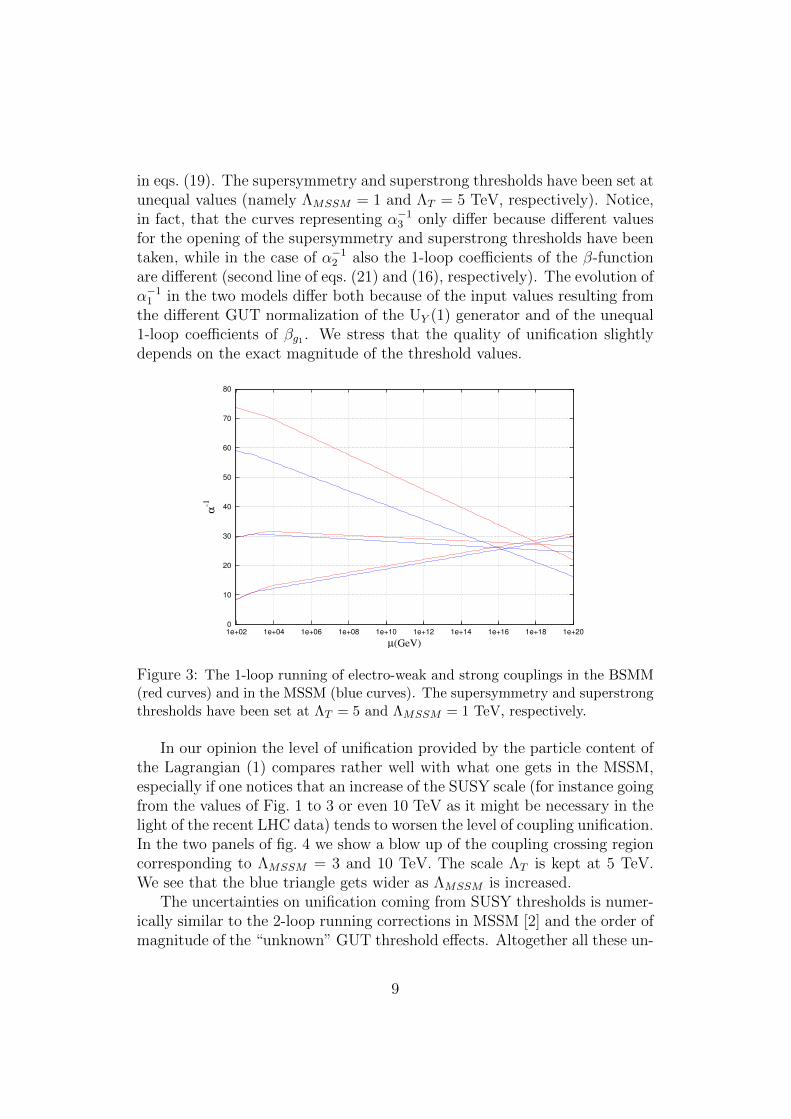
in eqs. (19). The supersymmetry and superstrong thresholds have been set atunequal values (namely ΛMSSM = 1 and ΛT = 5 TeV, respectively). Notice,in fact, that the curves representing α−13 only differ because different valuesfor the opening of the supersymmetry and superstrong thresholds have beentaken, while in the case of α−12 also the 1-loop coefficients of the β-functionare different (second line of eqs. (21) and (16), respectively). The evolution ofα−11 in the two models differ both because of the input values resulting fromthe different GUT normalization of the UY (1) generator and of the unequal1-loop coefficients of βg1 . We stress that the quality of unification slightlydepends on the exact magnitude of the threshold values.

0

10

20

30

40

50

60

70

80

1e+02 1e+04 1e+06 1e+08 1e+10 1e+12 1e+14 1e+16 1e+18 1e+20

α-1

µ(GeV)

Figure 3: The 1-loop running of electro-weak and strong couplings in the BSMM(red curves) and in the MSSM (blue curves). The supersymmetry and superstrongthresholds have been set at ΛT = 5 and ΛMSSM = 1 TeV, respectively.

In our opinion the level of unification provided by the particle content ofthe Lagrangian (1) compares rather well with what one gets in the MSSM,especially if one notices that an increase of the SUSY scale (for instance goingfrom the values of Fig. 1 to 3 or even 10 TeV as it might be necessary in thelight of the recent LHC data) tends to worsen the level of coupling unification.In the two panels of fig. 4 we show a blow up of the coupling crossing regioncorresponding to ΛMSSM = 3 and 10 TeV. The scale ΛT is kept at 5 TeV.We see that the blue triangle gets wider as ΛMSSM is increased.

The uncertainties on unification coming from SUSY thresholds is numer-ically similar to the 2-loop running corrections in MSSM [2] and the order ofmagnitude of the “unknown” GUT threshold effects. Altogether all these un-

9

certainties make difficult to predict the value of the unified inverse couplingwith an absolute accuracy better than one unit.

0

10

20

30

40

50

60

70

80

1e+02 1e+04 1e+06 1e+08 1e+10 1e+12 1e+14 1e+16 1e+18 1e+20

_-1

µ(GeV)

0

10

20

30

40

50

60

70

80

1e+02 1e+04 1e+06 1e+08 1e+10 1e+12 1e+14 1e+16 1e+18 1e+20

_-1

µ(GeV)Figure 4: The 1-loop running of electro-weak and strong couplings in the BSMM(red curves) and in the MSSM (blue curves). The supersymmetry thresholds havebeen set at ΛMSSM = 3 (left panel) and ΛMSSM = 10 TeV (right panel). Thescale ΛT relevant for the BSMM curves is kept at 5 TeV. The dashed grid is thesame as in fig. 3.

4.1 Observations

We conclude this section with a few observations.

4.1.1 Hypercharge assignments

The hypercharge assignment in Table 2 is the one for which Weinberg [3]writes that it “resembles nothing observed in nature”. The reason for taking

10

it for the hypercharges of SIPs is that with the more standard choice ofTable 1 one would not get a unification as good as the one visible in fig. 3.The difference is evident in fig. 5 where we compare the runnings that inthe BSMM are produced with the two types of hypercharge assignments.Clearly no unification can be achieved if the green curve, corresponding tothe Table 1 assignment, describes the one-loop running of α−11 .

It must be noticed that the hypercharge assignment of Table 2 yields Qand L elementary particles with electric charges ±e/2, hence superstronglyconfined “hadrons” have electrical charge quantized in units of e/2.

0

10

20

30

40

50

60

70

80

1e+02 1e+04 1e+06 1e+08 1e+10 1e+12 1e+14 1e+16 1e+18 1e+20

α-1

µ(GeV)

Figure 5: The 1-loop running of electro-weak and strong couplings in the BSMMwith the hyperchage assignment of Table 2 (red curves) and with the hyperchageassignment of Table 1 (green curve).

4.1.2 2-loop β-functions & threshold effects

We have extended the calculations of all the β-functions to 2-loops [14]. Wedo not report the corresponding (rather cumbersome) formulae here because2-loop terms do not modify in any essential way the previous plots, hence thequality of unification of gauge couplings visible in fig. 2. We recall that at2-loops the RG equations become much more involved as the RG evolutionof each coupling depends on all the others.

As we do not know what the full UV completion of the fundamentaltheory (1) could be, and consistently with our decision of (momentarily)neglecting 2-loop terms, we refrain from giving estimates of possible effectsdue threshold opening of GUT degrees of freedom around the GUT scale.

11

In any case 2-loop corrections and threshold effects tend to be of compa-rable numerical magnitude and may affect the values of the inverse couplingat (around) the unification scale at the level of about one unit.

4.1.3 Unification with superstrong interactions

A very indirect clue on the UV structure of the GUT theory can come fromthe interesting observation that unification of all the four gauge couplings[UY (1), SUL(2), SU(Nc = 3) and SU(NT = 3)] can be achieved if a certainnumber, NS, of purely SIPs are included in the model (1) with a Lagrangian

of the form∑NSh=1

(ψh 6DGψh +mhψ

hψh), where mh is an O(ΛGUT ) mass scale.

The presence of NS extra particles with purely superstrong vector inter-actions modifies the last formulae in eqs. (8) and (9) that become

Tr

[(1

2gTλ

3T

)2]

= [2(νL + νQNc) +NS]g2T , (22)

and (by setting Nc = NT = ng = 3 as well as νQ = νL = 1)

g24 =(

8 +NS

12

)g2T . (23)

This implies a modification of βg4 in eq. (16) that now reads

βg4 = −17

3

(12

8 +NS

)g34

(4π)2. (24)

It is remarkable that (approximate) unification of all the four couplings canbe achieved with reasonable values of NS (in the range between 4 and 6) andthe natural choice for the initial condition of α4

α−14 (µ = 5 TeV) = 1 . (25)

The situation is displayed in fig. 6 where the cases NS = 4 (blue line), NS = 5(black line) and NS = 6 (green line) are reported.

5 On the model of eq. (1)

The inspiration for the model (1) came from the work of ref. [4] (see alsoref. [5] for an earlier version of the investigation) where a non-perturbativeorigin for elementary particle masses, that does not rely on the Higgs mech-anism, was proposed. The complete Lagrangian of the model of ref. [4] (and

12

0

10

20

30

40

50

60

70

80

1e+02 1e+04 1e+06 1e+08 1e+10 1e+12 1e+14 1e+16 1e+18 1e+20

α-1

µ(GeV)

Figure 6: The 1-loop running of electro-weak strong and superstrong couplingsin the BSMM with the hyperchage assignment of Table 2 and NS = 4 (blue line)NS = 5 (black line), NS = 6 (green line).

its extension including electro-weak (EW) interactions [6]) involves a scalarSU(2) field coupled to fermions via chiral breaking Yukawa and Wilson-liketerms, the latter being “irrelevant” operators of dimension d = 6 appearingin the Lagrangian multiplied by two powers of the inverse UV cutoff. Thestructure of these terms is such that the whole Lagrangian (that is formallypower-counting renormalizable) enjoys an SUL(2)×UY (1) symmetry (underwhich all particles transform), crucial to forbid power divergent mass contri-butions in perturbation theory.

The complete model Lagrangian is not invariant, however, under chiralSUL(2)×UY (1) transformations of fermions and electroweak bosons only, butone can tune some parameters (the Yukawa coupling and the coefficientsof the Wilson-like terms) to critical values at which the symmetry of theLagrangian under these transformations is enforced up to UV cutoff effects,thus providing a solution of the naturalness problem in the way advocatedby ’t Hooft [7]. In the Nambu–Goldstone phase of the model elementaryparticle masses result from the non-perturbative spontaneous breaking ofthe restored chiral symmetry triggered by the (UV cutoff remnant of the)chiral symmetry breaking terms in the critical Lagrangian.

The elementary particle masses turn out to be proportional to the renor-malization group invariant (RGI) scale of the theory times powers of thecoupling constant of the strongest interactions which the particle is sub-

13

jected to. This means in particular that in order to get the right order ofmagnitude for the top mass the RGI scale of the whole theory must be muchlarger than ΛQCD. This is the reason why a new superstrongly interactingsector of particles (Q, L and gauge bosons), gauge invariantly coupled to SMmatter (q and `) as in eq. (1), is postulated to exist at a few TeV scale 2.

6 Conclusions

In this short note we have shown that it is possible to build non supersym-metric models (see, as an example, eq. (1)) where the unification of couplingsis realized to a level comparable to the one it is achieved in the MSSM andin any case much better that in the SM.

The salient feature of the BSMM described by the Lagrangian (1) is thepresence of a sector of superstrongly interacting (gluon-, quark- and lepton-like) particles with a ΛT � ΛQCD RGI scale set in the few TeV region.Superstrongly interacting fermions are endowed with a somewhat unusualhypercharge assignment implying that the confined states have the electriccharge quantized in units of e/2. Neutral bound states of SIPs with non-zerofermion number may provide candidates for cold dark matter along the linesdiscussed for techni-color, see e.g. in [15].

The motivation for studying the model (1) stems from the work of ref. [4]where it is conjectured that masses of elementary particles are generated in anon-perturbative way if a (small) chiral symmetry breaking seed is present inthe fundamental Lagrangian. The structure of the complete basic model ofrefs. [4, 6] is dictated by two key conceptual and phenomenological require-ments, namely a neat solution of the “naturalness” problem and the correctorder of magnitude of the dynamically generated top quark mass.

2We might suggestively call these new degrees of freedom “techni-particles” with aneye to well known techni-color models of refs. [8, 9]. We refrain from doing so as theframework underlying eq. (1) is very different from standard techni-color. One differenceis the absence of non-loop suppressed FCNC [6]. Another is that, unlike what happensin standard techni-color where techni-quarks are massless particles, our superstronglyinteracting particles (SIPs) have non-perturbatively generated masses of O(ΛT ) timesfactors of the superstrong coupling constant. In the model described by the Lagrangian (1)(with νQ = νL = 1) meson-like confined states will have masses that we can estimate, onthe basis of what happens in QCD, to be of the order of two or three times ΛT . Thisremark is important in the light of the existing bounds on the parameter S [10, 11] thattend to rule out standard techni-color with more than one doublet of techni-fermions. Thisis not so for the particle content of the model (1) because, as we have argued above, SIPconfined states have masses definitely “larger” than in standard techni-color, a fact thatsubstantially reduces their contributions to S.

14

References

[1] S. Dimopoulos, S. Raby and F. Wilczek, Phys. Rev. D 24 (1981) 1681.

[2] S. P. Martin, Adv. Ser. Direct. High Energy Phys. 21 (2010) 1 [Adv.Ser. Direct. High Energy Phys. 18 (1998) 1] [hep-ph/9709356].

[3] S. Weinberg, ”The Quantum Theory of Fields”, Vol. II, Cambridge Uni-versity Press (Cambridge, UK, 1995).

[4] R. Frezzotti and G. C. Rossi, Phys. Rev. D 92 (2015) 5, 054505.

[5] R. Frezzotti and G. C. Rossi, PoS LATTICE 2013 (2014) 354:

[6] R. Frezzotti and G. C. Rossi, in preparation.

[7] G. ’t Hooft, “Naturalness, Chiral Symmetry and Spontaneous ChiralSymmetry Breaking”, in “Recent Developments in Gauge Theories”(Plenum Press, 1980) - ISBN 978-0-306-40479-5.

[8] S. Weinberg, Phys. Rev. D 19 (1979) 1277-1280.

[9] L. Susskind, Phys. Rev. D 20 (1979) 2619-2625.

[10] M. E. Peskin and T. Takeuchi, Phys. Rev. Lett. 65 (1990) 964.

[11] M. E. Peskin and T. Takeuchi, Phys. Rev. D 46, 381 (1992).

[12] M. E. Machacek and M. T. Vaughn, Nucl. Phys. B 222 (1983) 83.

[13] K. A. Olive et al. (PDG), Chin. Phys. C 38 (2014) 090001.

[14] M. Garofalo, Master thesis, unpublished.

[15] J. Bagnasco, M. Dine and S. D. Thomas, Phys. Lett. B 320 (1994) 99.

15