Al '7 42 1 Vo 1 1O N OF NOW I IR WAVr fiOV " ONW 11IA WI VAR Y NG0 11F 1 U I I HN I NNi I'R R:";tl IA: oi,1A I A F A jI y c vI (; No RNI y F ;

Il( YiI 1 :AAP 8 ( 000

11251168 11.6

2.

AL1.4E

MICROCOPY~~ RESLUIO TES CAR

I IIIw LW '

ZVOLUMOII OF WOMLINKAR WAVZ CROUPS 01 WATER OF

SLOLY-VYARYDI DEPTH

Y. Frostig

Faculty of Civil Engineering

Technion - Israel Institute of Technology

CIO.,

Contract No. DAJA37-02-C-0300

Fourth Periodic Report, February 3983 - August 1983

The Research reported In this docummnt has bees madepossible through the support aad sponsorship of the U.S.Goverusnt through its European Research Office of theU.S. Army. This report is inteded only for the internal

asagement use of the contractor and the U.S. Governsent.

ITA

LA5 This docnatent hoem been approved FEB 1 184for public roleag. and sale; itsdistribution is unlimited.

__ _ 88 09 16 11r5

ti. ,

Work done during the regort Period

The Fourth periodical report concentrated on the

numerical solution of W.L.S. equation with varying coefficients.

The numerical treatment is based on the analytical

solution developed In the third periodical report. The solution

is valid using periodic boundaries end a very slow variation of

the bottom compared with the period's length. The solution was

compared with other numerical schemes and yield satisfactory

results.

All technical det ails are presented in the

following paper.

Dist Z,

-,, 1

YOLUTIGO 01 AN =STASI L I T WkV1 IUAIN X M 0M A SLWLY,

VARTEG BOTtO

(Part XI)

by t. lusts and . Froatig.

Introduction

--- The al of this paper is to present quantitative information

about the approximate solution of the nonlinear Schroedinger

i-4nAU.* quatlon with varying coefficients and periodic boundary

conditions d-sLe.J In M. -. (e ) compari g it

with merical solutions.

In section I ve present a brief review of the metbod developed -4

-is-42Yf-4" Nis based in t,, evaluation of an flnitial disturbec? "

at every poin aad local application of the analytical solution.,

gid--.mir-t u -(1-) In seet - os- qantitative

Information about the variation of the local initial disturbace A V1-

and As-swXLa-tt3~ w*e preseat the comparson of the solution

i fip GofbWt tmasritu solutions.

t. elviw of the Netbod te i the ItTdqiG %wort

The problem to be solved Is:

1* + #IT + ( 1)1 12 - 0 ( . )

vith the bom4ary condition

*0- 1 + 20eo(2 1 1) (1.2)

Name

-2-

Following Stiaalsi and Iroosynsky (1) we approximate ths solution

of (1.1), (1.2) by the truncated Fourier series:

S(T, 1 E D (X)e 2 IinT (1.3)

whore D n(X) io the complex Fourier coefficient of modulus Jj

and argument an:

- [Iin (.4)

The boundary condition at X - 0 implies that

JDo) - 1, %(o)- 0

(1.5)

ID1(o)D - a, -i(o) a a

From subetitution of (1.3) into the L.S. (1.1) the

following set of equation@ is obtained

IdD°

i 0 + (X) (Do1 2 + 41DI12)D0 + 2 ]" 0

(1.6)

i +(X) ((21Do12 + 31D112 - %i)Dl + DOD*,] - 0

where P bw2/M . The range of variation of P is I < P < 4. (see

Sticsnie, at al. (1)).

Assuming that the bottom varies so slowly that it may

be considered "locally constant". then the solution given by

Stiasmi et al. (1) for constant depth can be applied Locally.

This solution Is periodic In 2. Assmang that the bottom is "locally

constant" means that it is nearly constant in the period of the

solution.

Defining:

Z(X) - 21D 1(X)12 (1.7)

the exact solution of aystea (1.6) is given by the aet

Dol2 + Z - I + 2R3 (1.8)

coa2(so-) - i(P) +3/2 Z + [F-2(l+202)]Z (1.9)

ZZ(1+20--Z)

z(x) - Q (1.10)

s (-b) .. )c ) ((-d), adb r 11 a- ())" * -S)C - ) 2 da -(_ ) -b) a- c] (1.11)

(a-e(P))(b-d) (.-c)1

wbere cd M and sd represent the Jacobian elliptic functions

of argument

y- -J(7ab) 11X (1.12)

and modulus k given by

4 -1 k c-d)(.3(a-c) (b-d)O. )

a - 1 (l +C I + 21-(P)-P (1.14)

b -!4(1+2S2)-pJ 1 [1- 14I(P+)-

7 -P

C&, 11

-4-

4(1+2sz).P ]? } (1.16)

d - P (1- [I + 21(P)]1

if 1(P) > 0 or vice-versa, d given by (1.16) and c by (1.17) if

1(P) < 0.

The approximate solution depends on tvo parameters: I(P) and the

local Initial condition for Z: e(P). Given I(P) and C(P), Z(X) is

determined from (1.8) to (1.17). At the case of constant depth:

E(P) 3 coast - 262 (1.18)

and I(P) - conast - .2[ 202 + 4(1 + cos 2) - 2P] (1.19)

Under the asumption that the bottom is "locally constant"

In the some previously mentioned, we derived in (2) the folloving

approximate differential equation for I(P).

2 In( )

31(P) 47 T V 7P (1.20)

.n 1 -x~x 2

with the Initial condition (1.19).

-5-

Equation (1.20) can be easily solved aumerically.

In order to derive equation (1.20) we assumed in that the initial

condition of Z(X) for local disturbance satisfies the condition

c - a(P) - 1. we have chosen as the Local initial condition

E(P), the minimal positive value of the oxcilatory, function Z(X),

The minimal value of Z(X) Is found by equalling to zero its

derivative given by

az 3 2x - ,j~2Z(1+B-) 2 . iZ4P-2(1+202)]Z - 1(P)]2 (1.21)

(sea Stiassnie at &1. (1)).

If 1(P) 0 the minimal positive value of Z Is given by

C(P) - 4[4(1+202)_p] ( 1 141(P) c (1227 4(1+282)-p

and from (1.9) it can be seen that it correspond. to cos2(a0-a i =

If 1(P) < 0 the minimal positive value of Z is given by

C (P) P ( i - 1 I+ 21(P C (1.23)P2

and it corresponds to cos 2 (a o-a )-.

The approximate wave enveLope4' l(T,1Q is given by

1221*112 - (-21(P) + 2[4(1+202)-P]Z - 7Z2 +

+ CS (21(P) + 2PZ-Z 2 if + 4Zcos2irTJ2 1 /82. (1.24)

where 8 is the sign of cos(a1-o

-6-

11. The behavior of I(P)

The right hand side of equation (1.20) is alvays negative for the

range of values of P considerated 1 < P < 4, yieldlng that I(P) is a

decreasing function of P. On the other hand, it can be easily seen that

1(P) C.O is a solution of equation (1.20). That means that if the initial

condition I(P ) is positive, the solution remains positive, and

asinptotic to the horizontal axis. If the initial condition is

negative, the solution remains negative. The expected behavior of the solution

is given in figure. 1.

Figure 1

101

p¢

:J2

-7-

If I(P) - 0 then eqs. (1.16) and (1.17) yield c d 0 and

from (.13) we obtain k - 1. Then the period of the elliptic

functions in (1.11) is infinite (see (3)).

The solution Z(X) in this case is given by (1.10) where

1 a-b . tihV

Q -5 Y] (2.1)

+a-cb eh 2 y

where a and b are given by (1.14) and (1.15) respectively. From4. 10) and

(2.1) it can be seen that Z(X)-O(c). This solution is unstable to

disturbances in the parameter I(P), giving rise to the oscillatory

solution (l.lC),(l.ll) which grow.q from its minimal value Z = c - O(C),

to its maximal value z - b.

For this reason all the numerical calculations are unstable

near the value 1(P) - 0. On the other hand, when I(P) tends to zero,

the period of the oscillatory solution Z(X) tends to infinity, and

then our assumption that the bottom is nearly constant in a period

of the solution does not hold any more.

These reasons impose new restrictions in P. The permissible range

of variation of P must ensure the conditions II(P)l >> 1, but I(P)

not nearly zero.

From the numerical results we actually impose the condition

The solution of equation (1.20) is compared with the one

obtained by solving numerically the set (1.6) and using the

equality

1(P) - D12 [2jD112+4jD 0P2-2P4410 012cos2(c-4)A (2.2)

Equation (1.16) was solved by means of the second order RungeI

Kutta method, and by the trapezoidal rule, obtaining identical results.

System (1.6) was solved by the trapezoidal rule. In both cases

we considered the simple case wuhere P is linear on X:

P - P 0 + O.lx; P0 - 2 starting at X - 0. The results are presented

in figure 2. Full lines represent the solutions obtained

by (1.6) and (2.2), while dotted lines are the results from

numerical solutions of equation (1.20).x

I A

I-

.... - I -4 - J --V-- 0: 7... .. ... T , I

... ...... .....

H. I i ... ....Lo~~~~~~ ~ ~ ~ ~ I.....I ..I .. ::; ; .: . - ...I.......

1.0 t

s*

-10-

III. Comparison between the solution presented in section I

and numerical solutions

In order to appraise the validity of the behavior predicted

by equation (1.20) and the analytical solution (1.7) to (1.17), we

compare it with a reference solution obtained by means of numerical

schemes. In the first place we compare it with the numerical

solution of the set (1.6) obtained by means of the trapezoidal

rule. Figures 3 and 4 show the wave envelope 1*(OX) for the case

P - P + 0.lX, Po - 2, a - 0, 8 - 0.1.

These values correspond to the initial condition I(Po ) 0 0.0402.

Full lines represent the solutiun of the set (1.6) while dotted lines

are the results obtained by solving equation (1.20) and applying

(1.22), (1.11) to (1.17) and (1.24) at P - 2, P - 0.5 and P - 2.16.

Figures 5 and 6 represent the wave envelope I(O,T when a - %/2,

0 - 0.1 P P04.L, Po = 2, (I(po) - -0.0998). The full lines

represent the solution of set (1.6), and the dotted ones the

solution given by (1.20), (1.23), (1.10) to (1.17) and (1.24) at

P = 2 and P - 2.5. In boh cases a very satisfactory correspondence

of the wave envelop's shape is observed.

On the other hand, the solution of set (1.6) is compared

to the numerical solution of the N.L.S. equation when P - 2 + O.AX.

In order to solve the N.L.S. equation two independent alternative

numerical schemes were employed, obtaining identical results.

The first one is the Crank Nicholson scheme

. . .L

1' -11-J

n~~~l~ n- + ~2 e j +*.l + !L 2, O~

Ax (AT) 2 (AT) 2

+ V 4,1 on; -u Q (3.1)

where e -*(Tj,X n m' - 1(X), Tj - (J-I)LT, X = nAX, AT are

J-I equal segments that span the interval 0 < T < !i and AX are equal

intervals that span the X coordinate. The scheme is subject to then n

initial condition (1.2) and to the boundary conditions *o . n

n I n

J+ J J-1"

In the second approach wc seek an approximate solution of the

form

N

4P (T,X) - I D (X)e 2 snT (3.2)

Given the set #N(Tj,X) I -(N-),..,,,...N, the corresponding

Fourier coefficientsD(x,_l)...., DX) ,. .., DN(x) are found by means

of the Fast Fourier Transform, and conversely, given D(N-I) (x),...,

DO0,..,!N(x) the set ON(T X;=-(N-),..,O,1,..,N is found by means

of the Inverse Fourier Transform.

Substitution of (3.2) in the N.L.S. equation (1.1) yields:

idD+ i(2wn)2D - iVA 0 (3.3)

D - Dn (n -0,l,...,N)

where An - A (X), n - -(N-1),..,0,.,3 are the Fourier coefficients

of the set

IN(T X)12.*N(TJ,X), j -

A. ___,=2 .....- " " 22-z.. _ __

; -- 7

II ii i I lm I ll ii

iF

-12-

The solution of (3.1) i gives by

D+ (x) - ED {() + L A W(t)e (2wn)2tdt] 0-(2vi)2x (3.4)

which can be rewritten In the form

Djn(X+X) - D n(x) +tpe- l (2wn) 2x

IMAX

e L2vn)2tA(t)dt] a- Wn)X2 Aix

(3.7)

D n+A(z) + Afn (X) +AX e X (A +L(2wn) 2 (tXdt (3.6)x

Substitution of (3.6)into (3.5) leads to the numerical scheme

Do0(X+AX) - Do0 M + AXLu(Ao0 Wax) + Ao0(X*2

(3.7)

D*.(X+AX) - f.n (X) + (1-f.)(A n(X+AX)+A ft(X))/(P. 2)

n - 1,2,...,N

where f - •-i(2sn) 2AX

n

Starting with the known values of D at level X, we proceed

to compute A(X) by ases of the Fast Fourier Transform. We use this

valus " a first puess for A (X+X) and obtain an estimate for D (X+A1)

ftra (3.7). The Feet Fourier Transform and expression (3.7) are then

-13-

applied iteratively until no change between two successive estimates

are detected. The process is then advanced a further step in X. The first

step uses as starting values the initial condition (1.2).

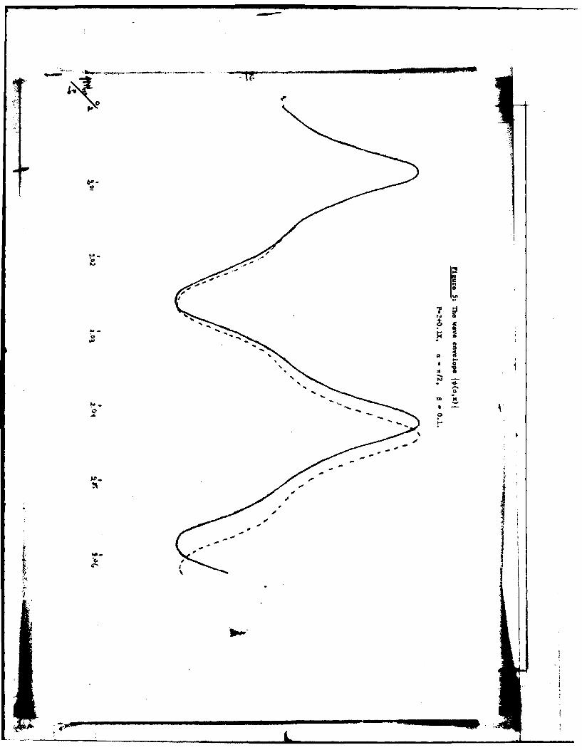
Figures 7 and 8 show the solution of the N.L.S. equation when

P - Po + 0.lX, Po - 2, for the initial conditions n- 0, B - 0.1

(UP )-0.0402) and a- 0, 0- 0.05 (I(Po ) - 0.01000125) respectively,0 0

while in figures 9 and 10 it can be seen the solution for the initial

conditions a - w/2, B - 0.1 (I(Po ) -0.0998), Full lines in these0Ifigures represent the solution of the N.L.S. equation, while dotted lines

represent the solution of system (1.6).

I,!

-vI-

0

p. I

9..a

*0V.

* 04* .I-. 4

4~ -S

05, - Uo N

I-.

o'I'

5-

- - - I

So - - -r-.

S.V

4.* .5

4.

I -

t~.

a

4~e-

6'

4a0

':3

4

a.9,

* -WY

*0 . w~. I,

0

aP.'

N

S

I-£ 0

Pd -

* 40

~ *4I.-0

'a-

1'

6~*

- -

I-

'-4

* 0

0 BI-

£ 0.4 *0

~ *

6 0

C N

4- -

'I

4.-. i

I- -

[4 I..

~50

34* 0~

'5.

* .-S

I

-

A'a.

I d.

'a 1* ..

---. I,jt 6

14 . .........

4-f

FlstaO 9: Tb* wave envelope

P - 240.11. ~ - 42. * - 0.1V

/ *

j

I

/

I/I/

II

I4 I

I I

C4 5

I

~ a

C -

I p j.olq

t

Figure 10: The vave envelope I*(a,x)jI

P.-2+0.11, a =W/2, 6-0.1

. - I

I p

ii

i//

p d

- " |alI

I

DATE

ILMED