Embed Size (px)
Citation preview
IS - New CFD methods for marine hydrodynamicsA new Volume-of-Fluid method in OpenFOAM
VII International Conference on Computational Methods in Marine EngineeringMARINE 2017
M. Visonneau, P. Queutey and D. Le Touze (Eds)
A NEW VOLUME-OF-FLUID METHOD IN OPENFOAM
Johan Roenby∗, Bjarke Eltard Larsen⋆, Henrik Bredmose† AND HrvojeJasak‡
∗DHI, Agern All 5, 2970 Hørsholm, Denmark, e-mail: [email protected]⋆DTU Mechanical Engineering, Richard Petersens Plads, 2800 Kgs. Lyngby, Denmark, e-mail:
[email protected]† DTU Wind Energy, Technical University of Denmark, Nils Koppels Alle, 2800 Lyngby,
Denmark‡Faculty of Mechanical Engineering and Naval Architecture, University of Zagreb, Ivana
Lucica 5, Zagreb, Croatia
Key words: CFD, Marine Engineering, Interfacial Flows, IsoAdvector, VOF Methods, SurfaceGravity Waves
Abstract. To realise the full potential of Computational Fluid Dynamics (CFD) within ma-rine science and engineering, there is a need for continuous maturing as well as verificationand validation of the numerical methods used for free surface and interfacial flows. One of thedistinguishing features here is the existence of a water surface undergoing large deformationsand topological changes during transient simulations e.g. of a breaking wave hitting an off-shore structure. To date, the most successful method for advecting the water surface in marineapplications is the Volume-of-Fluid (VOF) method. While VOF methods have become quiteadvanced and accurate on structured meshes, there is still room for improvement when it comesto unstructured meshes of the type needed to simulate flows in and around complex geometricstructures. We have recently developed a new geometric VOF algorithm called isoAdvector forgeneral meshes and implemented it in the OpenFOAM interfacial flow solver called interFoam.We have previously shown the advantages of isoAdvector for simple pure advection test caseson various mesh types. Here we test the effect of replacing the existing interface advectionmethod in interFoam, based on MULES limited interface compression, with the new isoAd-vector method. Our test case is a steady 2D stream function wave propagating in a periodicdomain. Based on a series of simulations with different numerical settings, we conclude that theintroduction of isoAdvector has a significant effect on wave propagation with interFoam. Thereare several criteria of success: Preservation of water volume, of interface sharpness and shape,of crest kinematics and celerity, not to mention computational efficiency. We demonstrate howisoAdvector can improve on many of these parameters, but also that the success depends on thesolver setup. Thus, we cautiously conclude that isoAdvector is a viable alternative to MULESwhen set up correctly, especially when interface sharpness, interface smoothness and calcula-tion times are important. There is, however, still potential for improvement in the coupling ofisoAdvector with interFoam’s PISO based pressure-velocity solution algorithm.
1
266
Johan Roenby, Bjarke Eltard Larsen, Henrik Bredmose and Hrvoje Jasak
1 INTRODUCTION
Computational Fluid Dynamics (CFD) is quickly gaining popularity as a tool for testing andoptimising marine structural designs and interaction with the surrounding water environment.A concrete example is the assessment of extreme wave loads on offshore wind turbine founda-tions of various types and shapes. From a numerical perspective, one of the great challengeswithin marine CFD is accurate description and advection of a complex free surface, or air-waterinterface. Various solution strategies have been developed to cope with this challenge[1]. Themost widely used within practical interfacial CFD is the Volume-of-Fluid (VOF) method. InVOF, the interface is indirectly represented by a numerical field describing the volume fractionof water within each computational cell. The game of VOF is then about “guessing” how muchwater is floating across the faces between adjacent cells within a time step. VOF methods comein two variants: 1) geometric VOF methods, using geometric operations to reconstruct the fluidinterface inside a cell and to approximate the water fluxes across faces, and 2) algebraic VOFmethods, relying on the limiter concept to blend first and higher order schemes in order toretain sharpness and boundedness of the time advanced VOF field. Geometric VOF schemes aretypically much more accurate, but also computationally more expensive, complex to implement,and restricted to certain types of computational meshes, such as hexahedral meshes. AlgebraicVOF schemes, on the other hand, are less accurate, but often faster, easier to implement, anddeveloped for general mesh types[2].
In marine applications, we often encounter complex geometries that are impossible, or atleast very difficult, to represent properly with a structured mesh. Hence, most free surface CFDwithin marine engineering is based on algebraic VOF methods. Therefore, such simulationsoften require excessive mesh resolution and therefore long calculation times to obtain the desiredsolution quality.
To address the need for an improved computational interface advection method, we havedeveloped a new VOF approach called IsoAdvector[3]. It is geometric of nature both in theinterface reconstruction and advection step, but is applicable on general meshes consisting ofarbitrary polyhedral cells. In the interface reconstruction, we take a novel approach usingisosurface calculations to find the interface position and orientation in the intersected cells. Inthe advection step, we rely on calculation of the face-interface intersection line sweeping a meshface during a time step. This avoids expensive calculations of intersections between cells andflux polyhedra[4]. For a thorough description of the isoAdvector concept the reader is referredto [3].
We have previously demonstrated using pure advection test cases that our new approachleads to accurate interface advection on both structured and unstructured meshes without com-promising calculation times[3]. In OpenFOAM’s interfacial flow solver, interFoam, each timestep starts by a MULES based update of the interface, followed by an update of the pressureand velocity, using a variant of the PISO algorithm[2]. In this segregated solution approachwe can simply remove the MULES code snippet and replace it by a corresponding isoAdvectorbased snippet. To complete the replacement of MULES with isoAdvector, we must also calculatethe mass flux across the faces – the quantity called rhoPhi in the interFoam code – based onisoAdvector, since this is needed in the convection term for the velocity field in construction andsolution of the discretised momentum equations. In [5], we show how to derive a simple expres-
2
267

Johan Roenby, Bjarke Eltard Larsen, Henrik Bredmose and Hrvoje Jasak
sion for rhoPhi from the mass fluxes provided by isoAdvector. The resulting solver is calledinterFlow and is provided as open source together with the isoAdvector library and various testcases at github.com/isoadvector.
In the following, we investigate the ability of interFlow and interFoam to propagate a streamfunction wave for 10 wave periods across a computational domain, which is exactly one wavelength long and has periodic boundary conditions on the sides.
Figure 1: The initial wave shape. The defining wave parameters are the water depth: D = 20m, wave height: H = 10 m, wave period: T = 14 s and mass transport velocity: u2 = 0 m/s.Some derived quantities are the wave length: L = 193.23 m, steepness: H/L = 0.052, celerity:c = 13.80 m/s, crest height: hcrest = 7.25 m, crest particle speed: ucrest = 5.95 m/s, troughheight: htrough = -2.75 m, trough particle speed: utrough = -2.25 m/s.
2 PHYSICAL SETUP
A stream function wave is a periodic steady wave calculated from potential flow theory usinga truncated Fourier expansion of the surface and stream function describing the wave. TheFourier coefficients are calculated using a numerical root finding method in parameter spaceand by growing the wave height in steps so the solution procedure can be seeded with an Airywave. For details on the solution procedure the reader is referred to [6]. Here we adopt thewave used in [7] and shown in Fig. 1, which also gives the wave parameters in the caption. Theadvantage of using stream function wave theory as opposed to Stokes N’th order theory for theinput wave is that the former does not rely on the smallness of the wave amplitude, which isthe Taylor expansion parameter of Stokes wave theory.
One thing to keep in mind, when attempting to reproduce potential theory waves in CFD isthat these waves are calculated under the assumption of a free surface, i.e. zero pressure andno air phase on top of the water surface. In our simulation we have a second phase above thewater and we are free to set the densities of the two phases. The water density will be set to1000 kg/m3. Ideally, we would like to set the air density to zero for our stream function testcase, but numerical stability issues limit how low we can set the air density. We choose an airdensity of 1 kg/m3, which is close to the real physical value. This is a good compromise, on onehand high enough to limit high density ratio related instabilities at the interface, and on theother hand low enough to make the air behaving like a “slave fluid” moving passively out of theway in response to motion of the much heavier water surface.
The viscosities in both phases is set to zero in accordance with potential flow theory and wehave deactivated the turbulence model. This amounts to running the solver in “Euler equation
3
268
Johan Roenby, Bjarke Eltard Larsen, Henrik Bredmose and Hrvoje Jasak
mode”, albeit the numerics will to some extend introduce an effective dissipation leading to alack of strict energy conservation.
For waves on the space and time scales considered here surface tension is irrelevant and weset it to zero in our simulations.
3 NUMERICAL SETUP
The interFoam and interFlow solvers used in this study are based on the OpenFOAM-v1612+version provided by ESI-OpenCFD. The details of the PISO algorithm implementation aredescribed in [2] and can be studied by inspecting the OpenFOAM code library, which is freelyavailable at openfoam.com.
For all simulations in the following the sides have periodic boundary conditions for both theVOF-field, α, the velocity field, U , and the pressure, p. On the top and bottom we have zeronormal gradient for α and p, and a slip boundary condition for U .
The mesh type with square cells and two refinement zones covering the interface region isshow in Fig. 1. This is the finest mesh used in this study with 20 cells per wave height and384 cells per wavelength in the interface region. Two coarser meshes with square cells were alsoused: One with the finest refinement removed, yielding 10 cells per wave height, and a verycoarse mesh with no refinement at all and only 5 cells per wave height.
In all simulations we use adaptive time stepping based on a maximum allowed CFL number.We show results with CFL = 0.1, 0.2 and 0.4. It should be noted that in water wave simulationswith interFoam the velocities in the air phase above the water surface are often higher thanthe maximum velocities in the water volume. The air behaviour depends a lot on the choicesof numerical schemes and settings, but for our density ratio of 1:1000, it is not uncommon tosee air velocities that are 2-3 times higher than the velocity of the water particles in the wavecrests. Thus, in a simulation with a maximum allowed CLF number of 0.1 the actual maximumCFL number in the water volume may in fact stay below 0.05. It might be fruitful to introducein the time stepping algorithm a separate CFL limit for each of the two phases.
Besides mesh and time resolution, the accuracy of wave propagation simulations dependson the choices of schemes for the different terms in the momentum equations. In particularthe results are sensitive to the choice of time integration scheme. Therefore, in what follows,we show results for both pure Euler time integration and a 50% mixture of Euler and Crank-Nicolson. Another influential scheme is the momentum convection scheme. The convective termis linearized and treated implicitly, so we use the face mass fluxes from a previous time step oriteration to advect the updated velocity field through the face. For the cell-to-face interpolationinvolved in the discretisation of the convective term we use a TVD method specialised for vectorfields, called limitedLinearV in OpenFOAM terminology. This scheme requires specification ofa coefficient in the range ψ ∈ [0, 1], where 0 gives best accuracy and 1 gives best convergence[8].In the following we use ψ = 1.
All discretisation schemes and solver settings used in the presented simulations are listed inAppendix A and B to allow the reader to verify our results.
4
269
270
Johan Roenby, Bjarke Eltard Larsen, Henrik Bredmose and Hrvoje Jasak
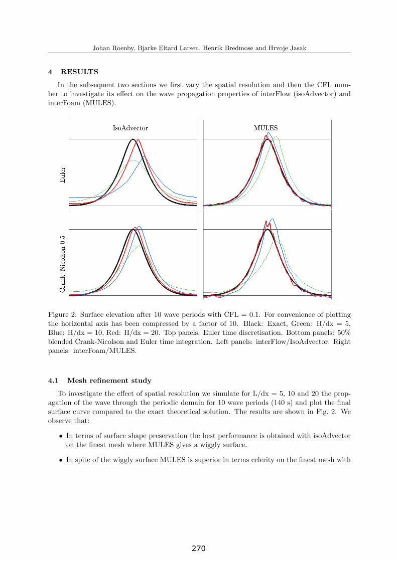
almost no visible phase shift.
• Using isoAdvector on the coarsest mesh leads to excessive decay in wave height.
• On the intermediate mesh isoAdvector also has excessive wave height decay with Eulerbut not with Crank-Nicolson.
• MULES with Euler looks surprisingly good on the coarsest mesh. Inspection of the timeseries reveals that this is a “lucky” snapshot right after the wave has broken due to excessivesteepening. In general it can not be recommended to use meshes with only 5 cells per waveheight with the numerical setup used here.
In Table 1 we show the time it took for the simulation of the 10 periods to finish on a singlecore for the different combinations of schemes and resolutions. IsoAdvector is significantly fasterthan MULES for all combinations except for the H/dx = 10 with Euler. For the best settings,H/dx=20 and Crank-Nicolson, isoAdvector is 32% faster than MULES and slightly faster thanthe MULES-Euler combination.
H/dx isoAdvector MULES
5 314 335
10 1892 1228
20 4356 5741
(a) Euler
H/dx isoAdvector MULES
5 304 435
10 918 1669
20 5624 8151
(b) Crank-Nicolson 0.5
Table 1: Simulation times in seconds on a single core for 10 periods.
4.2 Time refinement study
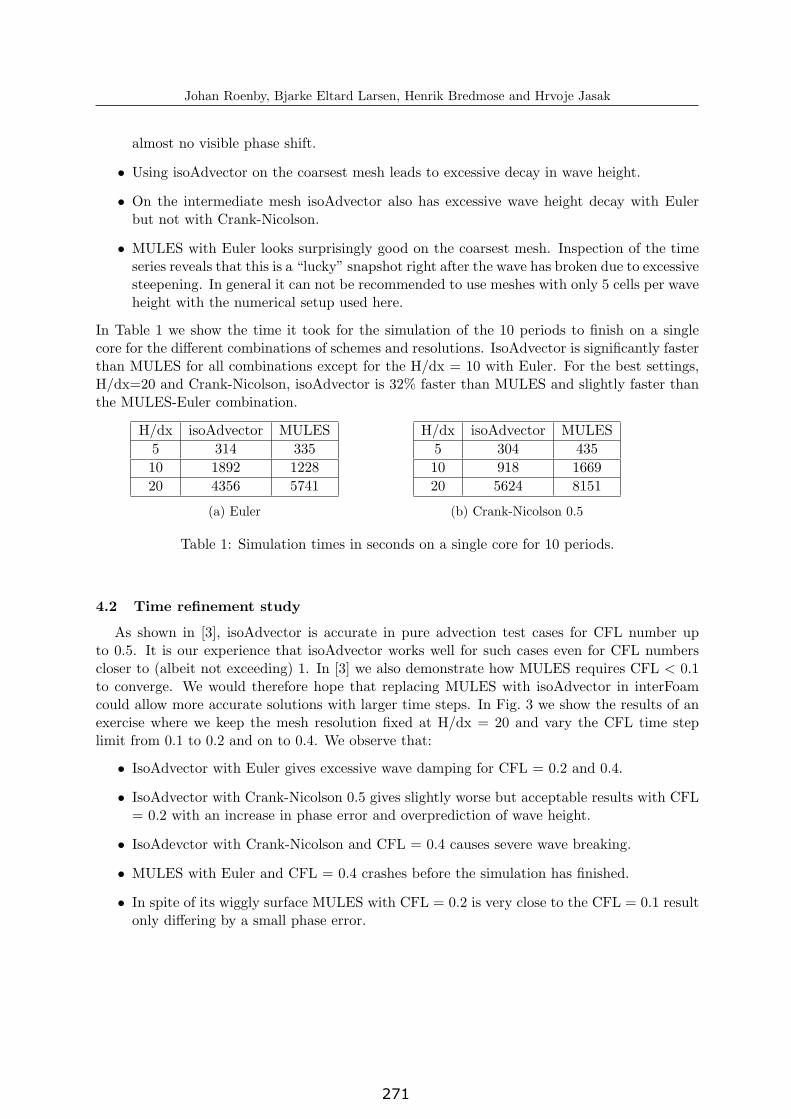
As shown in [3], isoAdvector is accurate in pure advection test cases for CFL number upto 0.5. It is our experience that isoAdvector works well for such cases even for CFL numberscloser to (albeit not exceeding) 1. In [3] we also demonstrate how MULES requires CFL < 0.1to converge. We would therefore hope that replacing MULES with isoAdvector in interFoamcould allow more accurate solutions with larger time steps. In Fig. 3 we show the results of anexercise where we keep the mesh resolution fixed at H/dx = 20 and vary the CFL time steplimit from 0.1 to 0.2 and on to 0.4. We observe that:
• IsoAdvector with Euler gives excessive wave damping for CFL = 0.2 and 0.4.
• IsoAdvector with Crank-Nicolson 0.5 gives slightly worse but acceptable results with CFL= 0.2 with an increase in phase error and overprediction of wave height.
• IsoAdevctor with Crank-Nicolson and CFL = 0.4 causes severe wave breaking.
• MULES with Euler and CFL = 0.4 crashes before the simulation has finished.
• In spite of its wiggly surface MULES with CFL = 0.2 is very close to the CFL = 0.1 resultonly differing by a small phase error.
6
271
272
Johan Roenby, Bjarke Eltard Larsen, Henrik Bredmose and Hrvoje Jasak
IsoAdvector
Euler
MULES
Crank–Nicolson0.5
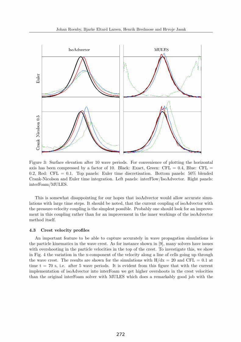
Figure 4: Horizontal velocity in cell centres at wave crest after 5 wave periods of the simulationwith H/dx = 20 and CFL = 0.1. Red: Exact, Green: Simulation result. The α-field is shownin a black-white colour map and the α = 0.001, 0.5 and 0.999 contours are plotted in blue. Toppanels: Euler time discretisation. Bottom panels: 50% blended Crank-Nicolson and Euler timeintegration. Left panels: interFlow/IsoAdvector. Right panels: interFoam/MULES.
Crank-Nicolson 0.5 time integration. Since the surface is advected passively in the velocity field,one should think that there was a strong correlation between a solver’s ability to represent thesevelocities accurately near the surface and its ability to accurately propagate the surface andpreserve its shape. This does not seem to be the case here where isoAdvector, in spite of itserrors in crest kinematics, produces a better surface, and MULES, in spite of its accurate crestkinematics, produces a wrinkled surface.
In Fig. 4, we show the interface width by plotting the α = 0.001, 0.5 and 0.999 contours in bluecolour. Careful inspection reveals that the distance between the 0.001 and 0.999 contours withisoAdvector is 3 which is essentially the theoretical minimal interface width for a VOF method.The corresponding distance with MULES is approximately twice as large, i.e. approximately 6cells. This moves the stagnation point, where the air velocity above the crest changes direction,
8
273
274
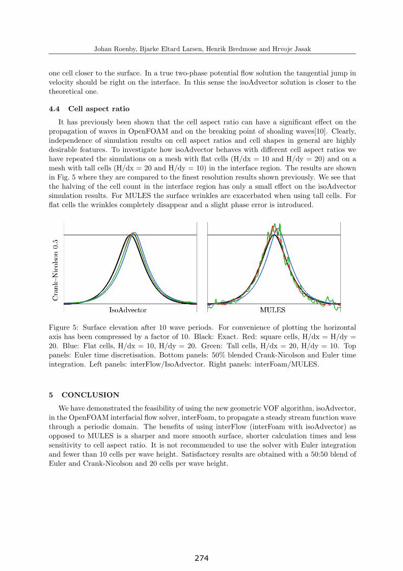
Johan Roenby, Bjarke Eltard Larsen, Henrik Bredmose and Hrvoje Jasak
In spite of problems with a wrinkly surface the original interFoam solver with MULES per-forms better than interFlow when it comes to phase error (celerity) on the finest mesh andreproduction of the theoretical crest kinematics profile. Also, at this stage interFlow does notproduce satisfactory results when running with CFL number > 0.2 as one might otherwise hopedue to its ability to advect interfaces accurately at CFL numbers close to 1. We expect thathigher accuracy at larger CFL numbers can be obtained by improving the way isoAdvector iscoupled with the PISO loop in the interFoam solver.
Finally a word of caution regarding this kind of numerical comparisons. Choosing schemesand solver settings is a delicate procedure which requires some degree of informed guessing. Itmay well be that one combination of schemes produces accurate results for a particular testcase because the energy that, say, the chosen time integration scheme erroneously injects intothe system is by pure luck equal to the energy erroneously taken out of the system due to thecoarseness of the mesh. Results may then look reasonable even though the numerical calculationdoes not in reality represent the simulated physics properly. A professional CFD engineer shouldalways stress test her setup with an attitude of trying to prove it wrong, rather than trying toprove it right.
Acknowledgements
This work was funded by JR’s Sapere Aude: DFF-Research Talent grant from The DanishCouncil for Independent Research | Technology and Production Sciences (Grant DFF-1337-00118) and by DHI’s GTS grant from the Danish Agency for Science, Technology and Innovation.
A Solver settings
PIMPLE isoAdvector
{ {
momentumPredictor yes; interfaceMethod isoAdvector;
nCorrectors 3; isoFaceTol 1e-8;
nOuterCorrectors 1; surfCellTol 1e-8;
nNonOrthogonalCorrectors 0; snapAlpha 1e-12;
nAlphaCorr 1; nAlphaBounds 3;
nAlphaSubCycles 1; clip true;
cAlpha 1; }
pRefPoint (1 0 16);
pRefValue 0;
}
"alpha.water.*" p_rgh
{ {
nAlphaCorr 2; solver GAMG;
nAlphaSubCycles 1; tolerance 1e-8;
cAlpha 1; relTol 0.01;
smoother DIC;
10
275
Johan Roenby, Bjarke Eltard Larsen, Henrik Bredmose and Hrvoje Jasak
MULESCorr no; nPreSweeps 0;
nLimiterIter 3; nPostSweeps 2;
nFinestSweeps 2;
solver smoothSolver; cacheAgglomeration true;
smoother symGaussSeidel; nCellsInCoarsestLevel 10;
tolerance 1e-8; agglomerator faceAreaPair;
relTol 0; mergeLevels 1;
} }
pcorr p_rghFinal
{ {
solver PCG; solver PCG;
preconditioner preconditioner
{ {
preconditioner GAMG; preconditioner GAMG;
tolerance 1e-5; tolerance 1e-8;
relTol 0; relTol 0;
smoother DICGaussSeidel; nVcycles 2;
nPreSweeps 0; smoother DICGaussSeidel;
nPostSweeps 2; nPreSweeps 2;
nFinestSweeps 2; nPostSweeps 2;
cacheAgglomeration false; nFinestSweeps 2;
nCellsInCoarsestLevel 10; cacheAgglomeration true;
agglomerator faceAreaPair; nCellsInCoarsestLevel 10;
mergeLevels 1; agglomerator faceAreaPair;
} mergeLevels 1;
tolerance 1e-06; }
relTol 0;
maxIter 100; tolerance 1e-9;
} relTol 0;
maxIter 20;
}
U UFinal
{ {
solver smoothSolver; solver smoothSolver;
smoother GaussSeidel; smoother GaussSeidel;
tolerance 1e-7; tolerance 1e-8;
relTol 0.05; relTol 0;
nSweeps 2; nSweeps 2;
} }
B Discretisation schemes
ddtSchemes{default CrankNicolson 0.5;} //Euler
11
276

Johan Roenby, Bjarke Eltard Larsen, Henrik Bredmose and Hrvoje Jasak
gradSchemes{default Gauss linear;}
divSchemes
{
div(rhoPhi,U) Gauss limitedLinearV 1;
div(phi,alpha) Gauss vanLeer;
div(phirb,alpha) Gauss interfaceCompression;
div(((rho*nuEff)*dev2(T(grad(U))))) Gauss linear;
}
laplacianSchemes{default Gauss linear corrected;}
interpolationSchemes{default linear;}
snGradSchemes{default corrected;}
REFERENCES
[1] G. Tryggvason, R. Scardovelli, and S. Zaleski, Direct numerical simulations of gas–liquid
multiphase flows. Cambridge University Press, 2011.
[2] S. S. Deshpande, L. Anumolu, and M. F. Trujillo, “Evaluating the performance of the two-phase flow solver interFoam,” Computational Science & Discovery, vol. 5, no. 1, p. 014016,2012.
[3] J. Roenby, H. Bredmose, and H. Jasak, “A computational method for sharp interface ad-vection,” Royal Society Open Science, vol. 3, no. 11, p. 160405, 2016.
[4] J. Hernandez, J. Lopez, P. Gomez, C. Zanzi, and F. Faura, “A new volume of fluid methodin three dimensions-part I: Multidimensional advection method with face-matched fluxpolyhedra,” International Journal for Numerical Methods in Fluids, vol. 58, no. 8, pp. 897–921, 2008.
[5] J. Roenby, H. Bredmose, and H. Jasak, “Isoadvector: Vof on general meshes,” in 11th Open-
FOAM Workshop (J. M. Nobrega and H. Jasak, eds.), Springer Nature, 2017. submitted.
[6] John D. Fenton, “Numerical methods for nonliner waves,” in Advances in Coastal and Ocean
Engineering, vol. 5, pp. 241–324, World Scientific, July 1999.
[7] B. T. Paulsen, H. Bredmose, H. Bingham, and N. Jacobsen, “Forcing of a bottom-mountedcircular cylinder by steep regular water waves at finite depth,” Journal of Fluid Mechanics,vol. 755, pp. 1–34, Sept. 2014.
[8] C. J. Greenshields, “Openfoam user guide,” OpenFOAM Foundation Ltd, version, vol. 3,no. 1, 2015.
[9] P. A. Wroniszewski, J. C. G. Verschaeve, and G. K. Pedersen, “Benchmarking of Navier-Stokes codes for free surface simulations by means of a solitary wave,” Coastal Engineering,vol. 91, pp. 1–17, Sept. 2014.
[10] N. G. Jacobsen, D. R. Fuhrman, and J. Fredsøe, “A wave generation toolbox for the open-source CFD library: OpenFoam,” International Journal for Numerical Methods in Fluids,vol. 70, no. 9, pp. 1073–1088, 2012.
12
277


![[302.044] Numerical Methods in Fluid Dynamics …info.tuwien.ac.at/ViennaOpenFOAMUserGroup/9thb... · OpenFOAM Tutorial Finite Volume Method, Dictionary ... francesco.romano@tuwien.ac.at](https://img.dokumen.tips/doc/110x75/5af822c97f8b9aff288b76a5/302044-numerical-methods-in-fluid-dynamics-info-tutorial-finite-volume-method.jpg)