Embed Size (px)
Citation preview

Hindawi Publishing CorporationJournal of Applied MathematicsVolume 2012, Article ID 542401, 19 pagesdoi:10.1155/2012/542401
Research ArticleWavelet Collocation Method for Solving MultiorderFractional Differential Equations
M. H. Heydari, M. R. Hooshmandasl, F. M. Maalek Ghaini,and F. Mohammadi
Faculty of Mathematics, Yazd University, Yazd, Iran
Correspondence should be addressed to M. R. Hooshmandasl, [email protected]
Received 15 July 2011; Accepted 27 October 2011
Academic Editor: Md. Sazzad Chowdhury
Copyright q 2012 M. H. Heydari et al. This is an open access article distributed under the CreativeCommons Attribution License, which permits unrestricted use, distribution, and reproduction inany medium, provided the original work is properly cited.
The operational matrices of fractional-order integration for the Legendre and Chebyshev waveletsare derived. Block pulse functions and collocation method are employed to derive a generalprocedure for forming these matrices for both the Legendre and the Chebyshev wavelets. Thennumerical methods based on wavelet expansion and these operational matrices are proposed. Inthis proposed method, by a change of variables, the multiorder fractional differential equations(MOFDEs) with nonhomogeneous initial conditions are transformed to the MOFDEs withhomogeneous initial conditions to obtain suitable numerical solution of these problems. Numericalexamples are provided to demonstrate the applicability and simplicity of the numerical schemebased on the Legendre and Chebyshev wavelets.
1. Introduction
Fractional-order differential equations (FODEs), as generalizations of classical integer-orderdifferential equations, are increasingly used tomodel some problems in fluid flow,mechanics,viscoelasticity, biology, physics, engineering, and other applications. Fractional derivativesprovide an excellent instrument for the description of memory and hereditary properties ofvarious materials and processes [1–6]. Fractional differentiation and integration operators arealso used for extensions of the diffusion and wave equations [7]. The solutions of FODEs aremuch involved, because in general, there exists no method that yields an exact solution forFODEs, and only approximate solutions can be derived using linearization or perturbationmethods. Several methods have been suggested to solve fractional differential equations(see [8] and references therein). Also there are different methods for solving MOFDEs asa special kind of FODEs [9–17]. However, few papers have reported applications of waveletsin solving fractional differential equations [8, 18–21]. In view of successful application of

2 Journal of Applied Mathematics
wavelet operational matrices in numerical solution of integral and differential equations [22–27], together with the characteristics of wavelet functions, we believe that they should beapplicable in solving MOFDEs.
In this paper, the operational matrices of fractional-order integrations are derived anda general procedure based on collocation method and block pulse functions for formingthese matrices is presented. Then, by application of these matrices, a numerical method forsolving MOFDEs with nonhomogeneous conditions is presented. In the proposed methodby a change of variables the MOFDEs with nonhomogeneous conditions transforms to theMOFDEs with homogeneous conditions. This way, we are able to obtain the exact solutionsfor such problems. In the proposedmethod, the Legendre andChebyshevwavelet expansionsalong with operational matrices of fractional-order integrations are employed to reducethe MOFDE to systems of nonlinear algebraic equations. Illustrative examples of nonlineartypes are given to demonstrate the efficiency and applicability of the proposed method. Asnumerical results show, the proposed method is efficient and simple in implementation forboth the Legendre and the Chebyshev wavelets. Moreover, for both these kinds of wavelets,numerical results have a good agreement with the exact solutions and the numerical resultspresented in other works.
The paper is organized as follows. In Section 2, we review some necessary definitionsand mathematical preliminaries of fractional calculus and wavelets that are required forestablishing our results. In Section 3 the Legendre and Chebyshev operational matricesof integration are derived. In Section 4 an application of the Legendre and Chebyshevoperational matrices for solving the MOFDEs is presented. In Section 5 the proposed methodis applied to several numerical examples. Finally, a conclusion is given in Section 6.
2. Basic Definitions
2.1. Fractional Calculus
We give some basic definitions and properties of the fractional calculus theory which are usedfurther in this paper.
Definition 2.1. A real function f(t), t > 0, is said to be in the space Cμ, μ ∈ R if there exists areal number p(> μ) such that f(t) = tpf1(t), where f1(t) ∈ C[0,∞], and it is said to be in thespace Cn
μ if f(n) ∈ Cμ, n ∈ N.
Definition 2.2. The Riemann-Liouville fractional integration operator of order α ≥ 0, of afunction f ∈ Cμ, μ ≥ −1, is defined as follows [4]:
Iαf(t) =1
Γ(α)
∫ t0(t − τ)α−1f(τ)dτ,
I0f(t) = f(t),(2.1)
and according to [4], we haveIαIβf(t) = Iα+βf(t),
IαIβf(t) = IβIαf(t),
Iαtϑ =Γ(ϑ + 1)
Γ(α + ϑ + 1)tα+ϑ,
(2.2)
where α, β ≥ 0, t > 0 and ϑ > −1.

Journal of Applied Mathematics 3
Definition 2.3. The fractional derivative of order α > 0 in the Riemann-Liouville sense isdefined as [4]
Dαf(t) =(d
dt
)nIn−αf(t), (n − 1 < α ≤ n), (2.3)
where n is an integer and f ∈ Cn1 .
The Riemann-Liouville derivatives have certain disadvantages when trying to modelreal-world phenomena with fractional differential equations. Therefore, we will now intro-duce a modified fractional differential operator Dα
∗ proposed by Caputo [5].
Definition 2.4. The fractional derivative of order α > 0 in the Caputo sense is defined as [5]
Dα∗f(t) =
1Γ(n − α)
∫ t0(t − τ)n−α−1f (n)(τ)dτ, (n − 1 < α ≤ n), (2.4)
where n is an integer t > 0 and f ∈ Cn1 . Caputos integral operator has a useful property:
IαDα∗f(t) = f(t) −
n−1∑k=0
f (k)(0+)tk
k!, (n − 1 < α ≤ n), (2.5)
where n is an integer t > 0 and f ∈ Cn1 .
2.2. Wavelets
Wavelets constitute a family of functions constructed from dilations and translations of asingle function called the mother wavelet ψ(t). When the dilation parameter a and thetranslation parameter b vary continuously, we have the following family of continuouswavelets [24]:
ψa,b(t) = |a|−1/2ψ(t − ba
), a, b ∈ R, a /= 0. (2.6)
If we restrict the parameters a and b to discrete values as a = a−k0 , b = nb0a−k0 , a0 > 1,
b0 > 0, for n and k positive integers, we have the following family of discrete wavelets:
ψk,n(t) = |a0|k/2ψ(ak0 t − nb0
), (2.7)
where ψk,n(t) forms a wavelet basis for L2(R). In particular, when a0 = 2 and b0 = 1, ψk,n(t)forms an orthonormal basis. That is (ψk,n(t), ψl,m(t)) = δklδnm.

4 Journal of Applied Mathematics
2.2.1. The Legendre Wavelets
The Legendre wavelets ψn,m(t) = ψ(k, n,m, t) have four arguments; k ∈ N, n = 1, 2, . . . , 2k−1,and n = 2n− 1; moreover,m is the order of the Legendre polynomials and t is the normalizedtime, and they are defined on the interval [0, 1) as
ψn,m(t) =
⎧⎪⎨⎪⎩
√m +
122k/2pm
(2kt − n), n − 1
2k≤ t < n
2k,
0, otherwise,(2.8)
where m = 0, 1, . . . ,M − 1 and M is a fixed positive integer. The coefficient√m + 1/2 in
(2.8) is for orthonormality, the dilation parameter is a = 2−k, and the translation parameteris b = n2−k. Here, Pm(t) are the well-known Legendre polynomials of order m which areorthogonal with respect to the weight functionw(t) = 1 on the interval [−1, 1] and satisfy thefollowing recursive formula:
p0(t) = 1, p1(t) = t, pm+1(t) =(2m + 1m + 1
)tpm(t) −
(m
m + 1
)pm−1(t), m = 1, 2, 3, . . . .
(2.9)
2.2.2. The Chebyshev Wavelets
The Chebyshev wavelets ψn,m(t) = ψ(k, n,m, t) have four arguments; k ∈ N, n = 1, 2, . . . , 2k−1,and n = 2n − 1; moreover,m is the order of the Chebyshev polynomials of the first kind and tis the normalized time, and they are defined on the interval [0, 1) as
ψn,m(t) =
⎧⎪⎨⎪⎩2k/2Tm
(2kt − n), n − 1
2k≤ t < n
2k,
0, otherwise,(2.10)
where
Tm(t) =
⎧⎪⎪⎪⎨⎪⎪⎪⎩
1√π, m = 0,
√2πTm(t), m > 0,
(2.11)
where m = 0, 1, . . . ,M − 1 and M is a fixed positive integer. The coefficients in (2.11) areused for orthonormality. Here, Tm(t) are the well-known Chebyshev polynomials of order mwhich are orthogonal with respect to the weight function w(t) = 1/
√1 − t2 on the interval
[−1, 1] and satisfy the following recursive formula:
T0(t) = 1, T1(t) = t, Tm+1(t) = 2tTm(t) − Tm−1, m = 1, 2, 3 . . . . (2.12)

Journal of Applied Mathematics 5
We should note that in dealing with the Chebyshev polynomials the weight function w =w(2t − 1) has to be dilated and translated as follows:
wn(t) = w(2kt − n
), (2.13)
to get orthogonal wavelets.
2.2.3. Function Approximation
A function f(t) defined over [0, 1) may be expanded as follows:
f(t) =∞∑n=1
∞∑m=0
cn,mψn,m(t), (2.14)
by the Legendre or Chebyshev wavelets, where cn,m = (f(t), ψn,m(t)) in which (, ) denotes theinner product.
If the infinite series in (2.14) is truncated, then (2.14) can be written as
f(t) ≈2k−1∑n=1
M−1∑m=0
cn,mψn,m(t) = CTΨ(t), (2.15)
where C and Ψ(t) are 2k−1M × 1 matrices given by
C = [c10, c11, . . . , c1M−1, c20, . . . , c2M−1, . . . , c2k−10, . . . , c2k−1M−1]T ,
Ψ =[ψ10(t), ψ11(t), . . . , ψ1M−1(t), ψ20(t), . . . , ψ2M−1(t), . . . , ψ2k−10(t), . . . , ψ2k−1M−1(t)
]T.
(2.16)
Taking the collocation points
ti =(2i − 1)2kM
, i = 1, 2, . . . , m, (2.17)
wherem = 2k−1M, we define the wavelet matrix Φm×m as
Φm×m =[Ψ(
12m
),Ψ(
32m
), . . . ,Ψ
(2m − 12m
)]. (2.18)
Indeed Φm×m has the following form:
Φm×m =
⎡⎢⎢⎢⎢⎢⎢⎣
A 0 · · · 0 00 A 0 · · · 00 0 A · · · 0...
.... . . . . .
...0 0 · · · 0 A
⎤⎥⎥⎥⎥⎥⎥⎦, (2.19)

6 Journal of Applied Mathematics
where A is aM ×M matrix given by
A =
⎡⎢⎢⎢⎢⎢⎢⎢⎢⎢⎢⎢⎣
ψ10
(12m
)ψ10
(32m
)· · · ψ10
(2M − 12m
)
ψ11
(12m
)ψ11
(32m
)· · · ψ11
(2M − 12m
)
......
......
ψ1M−1
(12m
)ψ1M−1
(32m
)· · · ψ1M−1
(2M − 12m
)
⎤⎥⎥⎥⎥⎥⎥⎥⎥⎥⎥⎥⎦
. (2.20)
For example, for M = 4 and k = 2, the Legendre and Chebyshev matrices can beexpressed as
Φ8 × 8 =[A 00 A
], (2.21)
where for the Legendre matrix we have
A =
⎡⎢⎢⎣
1.41421 1.41421 1.41421 1.41421−1.83712 −.612372 0.612372 1.837121.08703 −1.28468 −1.28468 1.087030.263085 1.25697 −1.25697 −.263085
⎤⎥⎥⎦, (2.22)
and for the Chebyshev matrix we have
A =
⎡⎢⎢⎣
1.12838 1.12838 1.12838 1.12838−1.19683 −.398942 −.398942 1.196830.199471 −1.39630 −1.39630 0.1994710.897621 1.09709 −1.09709 −.897621
⎤⎥⎥⎦. (2.23)
3. Operational Matrix of Fractional Integration
The integration of the vector Ψ(t) defined in (2.16) can be obtained by
∫ t0Ψ(τ)dτ ≈ PΨ(t), (3.1)
where P is them ×m operational matrix for integration [24].Now, we derive the wavelet operational matrix of fractional integration. For this
purpose, we rewrite the Riemann-Liouville fractional integration as
(Iαf)(t) =
1Γ(α)
∫ t0(t − τ)α−1f(τ)dτ =
1Γ(α)
tα−1 ∗ f(t), (3.2)

Journal of Applied Mathematics 7
where α ∈ R is the order of the integration and tα−1 ∗ f(t) denotes the convolution product oftα−1 and f(t). Now if f(t) is expanded by the Legendre and Chebyshev wavelets, as shownin (2.15), the Riemann-Liouville fractional integration becomes
(Iαf)(t) =
1Γ(α)
tα−1 ∗ f(t) ≈ CT 1Γ(α)
{tα−1 ∗Ψ(t)
}. (3.3)
So that, if tα−1 ∗ f(t) can be integrated, then by expanding f(t) in the Legendre andChebyshev wavelets, the Riemann-Liouville fractional integration can be solved via theLegendre and Chebyshev wavelets.
Also, we define anm-set of block pulse functions (BPFs) as
bi(t) =
⎧⎪⎨⎪⎩1,
i
m≤ t < (i + 1)
m,
0, otherwise,(3.4)
where i = 0, 1, 2, . . . , (m − 1).The functions bi(t) are disjoint and orthogonal, that is,
bi(t)bl(t) =
{0, i /= l,bi(t), i = l,
∫10bi(τ)bl(τ)dτ =
⎧⎪⎨⎪⎩0, i /= l,1m, i = l.
(3.5)
Similarly, the Legendre and Chebyshev wavelets may be expanded intom-term blockpulse functions (BPFs) as follows:
Ψm(t) = Φm×mBm(t), (3.6)
where Bm(t) = [b0(t), b1(t), . . . , bi(t), . . . , bm−1(t)]T .
In [28], Kilicman and Al Zhour have given the block pulse operational matrix of thefractional integration Fα as follows:
(IαBm)(t) ≈ FαBm(t), (3.7)
where
Fα =1mα
1Γ(α + 2)
⎡⎢⎢⎢⎢⎢⎢⎢⎢⎢⎣
1 ξ1 ξ2 · · · ξm−1
0 1 ξ1 · · · ξm−2
0 0 1 · · · ξm−3
0 0 0. . .
...
0 0 0 0 1
⎤⎥⎥⎥⎥⎥⎥⎥⎥⎥⎦, (3.8)

8 Journal of Applied Mathematics
and ξi = (i + 1)α+1 − 2iα+1 + (i − 1)α+1. Next, we derive the Legendre and Chebyshev waveletoperational matrices of the fractional integration. Let
(IαΨm)(t) ≈ Pαm×mΨm(t), (3.9)
where the matrix Pαm×m is called the wavelet operational matrix of the fractional integration.Using (3.6) and (3.7), we have
(IαΨm)(t) ≈ (IαΦm×mBm×m)(t) = Φm×m(IαBm)(t) ≈ Φm×mFαBm(t), (3.10)
and from (3.9) and (3.10), we get
Pαm×mΨm(t) ≈ Pαm×mΦm×mBm(t) ≈ Φm×mFαBm(t). (3.11)
Thus, the Legendre and Chebyshev wavelet operational matrices of the fractional inte-gration Pαm×m can be approximately expressed by
Pαm×m = Φm×mFαΦ−1m×m. (3.12)
Also, from (3.3) and (3.12), we obtain
(Iαf)(t) ≈ CTΦm×mFαBm(t). (3.13)
Here, for the Legendre and Chebyshev wavelets, we can obtain Φm×mFα as follows:
Φm×mFα =
⎡⎢⎢⎢⎢⎢⎢⎣
B1 B2 B3 · · · Bk0 B1 B2 · · · Bk−10 0 B1 · · · Bk−20 0 0
. . ....
0 0 0 0 B1
⎤⎥⎥⎥⎥⎥⎥⎦, (3.14)
where Br , r = 1, 2, . . . , k(k = 2k−1), areM ×Mmatrices given by
Br =(b(r)ij
)M×M
, (3.15)
such that for r = 1,
b(1)ij =
j∑l=1
ailξ′j−l, ξ′0 = 1, (3.16)

Journal of Applied Mathematics 9
and for r = 2, 3, . . . ,M,
Br =(b(r)ij
)M×M
, l = 2, 3, . . . , k,
b(r)ij =
M∑l=1
ailξ′(r−1)M−l+j ,
(3.17)
where
aij = Ψ1(i−1)
(2j − 12m
), (3.18)
and ξ′j = (1/mαΓ(α + 2))ξj , j = 0, 1, . . . m − 1.Now from (3.12) and (3.14), we have
Pαm×m =
⎡⎢⎢⎢⎢⎢⎢⎢⎢⎢⎣
D1 D2 D3 · · · Dk
0 D1 D2 · · · Dk−10 0 D1 · · · Dk−2
0 0 0. . .
...
0 0 0 0 D1
⎤⎥⎥⎥⎥⎥⎥⎥⎥⎥⎦, (3.19)
where Di = BiA−1, i = 1, 2, . . . k.
4. Applications and Results
In this section, the Legendre and Chebyshev wavelet expansions together with theiroperational matrices of fractional-order integration are used to obtain numerical solution ofMOFDEs.
Consider the following nonlinear MOFDE:
β0(t)Dα∗y(t) +
s1∑i=1
βi(t)Dαi∗ y(t) +
s2∑i=1
γi(t)yi(t) = f(t), y(j)(0) = cj , j = 0, 1, . . . n − 1,
(4.1)
where 0 ≤ t < 1, n − 1 < α ≤ n, 0 < α1 < α2 < · · · < αs1 < α, n, s1 and s2 are fixed positiveintegers, Dα
∗ denotes the Caputo fractional derivative of order α, f is a known function of t,cj , j = 0, 1, . . . , n − 1, are arbitrary constants, and y is an unknown function to be determinedlater. To solve this problem, we apply the following scheme.
Suppose
y(t) =n−1∑j=0
cjtj
j!+ Y (t). (4.2)

10 Journal of Applied Mathematics
Under this change of variable, we have
yi(t) =
⎛⎝n−1∑
j=0
cjtj
j!+ Y (t)
⎞⎠
i
=i∑
s=0
(is
)⎛⎝n−1∑j=0
cjtj
j!
⎞⎠
s
Y (t)i−s,
Dα∗y(t) = D
α∗Y (t),
Dαi∗ y(t) = Dαi∗ Y (t), n − 1 < αi < α,
Dαi∗ y(t) = Dαi∗ Y (t) + hi(t), αi ≤ n − 1,
(4.3)
where
hi(t) = Dαi∗
⎛⎝n−1∑
j=0
cjtj
j!
⎞⎠. (4.4)
Now, by substituting (4.3) into (4.1), we transform the nonlinear MOFDE (4.1) withnonhomogeneous conditions to a nonlinear MOFDE with homogeneous conditions as fol-lows:
β0(t)Dα∗Y (t)+
s1∑i=1
βi(t)Dαi∗ Y (t)+
s2∑i=1
i∑s=0
γi,s(t)Y i−s(t) = f(t), Y (j)(0) = 0, j = 0, 1, . . . n − 1,
(4.5)
where
β0(t) = β0(t),
βi(t) = βi(t), n − 1 < αi < α,
βi(t) = βi(t)hi(t), αi ≤ n − 1,
γi,s(t) = γi(t)(is
)⎛⎝n−1∑j=0
cjtj
j!
⎞⎠
s
,
(4.6)
and f(t) is a known function.We assume that Dα
∗Y (t) is given by
Dα∗Y (t) = K
TmΨm(t), (4.7)
where KTm is an unknown vector and Ψm(t) is the vector which is defined in (3.6). By using
initial conditions and (2.4), we have
Dαi∗ Y (t) = KTmP
α−αim×mΨm(t), i = 1, 2, . . . , s1, (4.8)
Y (t) = KTmP
αm×mΨm(t). (4.9)

Journal of Applied Mathematics 11
Since Ψm = Φm×mBm(t), (4.9) can be rewritten as follows:
Y (t) = KTmP
αm×mΦm×mBm(t) = [a1, a2, . . . , am]Bm(t). (4.10)
Now by using (3.4), we obtain
[Y (t)]i−s =[ai−s1 , ai−s2 , . . . , ai−sm
]Bm(t), i = 1, 2, . . . , s2, s = 0, 1, . . . , i. (4.11)
Moreover, we expand functions βi(t), γi,s(t), and f(t) by wavelets as follows:
βi(t) = Ψm(t)T βi,m, i = 0, 1, . . . , s1,
γi,s(t) = Ψm(t)T γi,s,m, i = 1, 2, . . . , s2, s = 0, 1, . . . , i,
f(t) = fTmΨm(t),
(4.12)
where βi,m, γi,m, and fTm are known vectors. By substituting (4.7), (4.8), and (4.11)-(4.12) into(4.5), we obtain
Ψm(t)T β0,mKTmΨm(t)+
s1∑i=1
Ψm(t)T βi,mKTmP
α−αim×mΨm(t)+
s2∑i=1
i∑s=0
Ψm(t)T γi,s,m[ai−s1 , ai−s2 , . . . , ai−sm
]Bm(t)
= Bm(t)T [1, 1, . . . , 1]TfTmΨm(t).(4.13)
Now, from (3.12), (4.10), and (4.13), we have
Bm(t)T[ΦTm×mβ0,m[a1, a2, . . . , am]F
α−1 +s1∑i=1
ΦTm×mβi,m[a1, a2, . . . , am]F
α−1Fαα−αi
+s2∑i=1
i∑s=0
ΦTm×mγi,s,m
[ai−s1 , ai−s2 , . . . , ai−sm
]]Bm(t) = Bm(t)T [1, 1, . . . , 1]TfTmΦm×mBm(t).
(4.14)
This is a nonlinear algebraic equation for unknown vector [a1, a2, . . . , am]. Here, bytaking collocation points, expressed in (2.17), we transform (4.14) into a nonlinear system ofalgebraic equations. This nonlinear system can be solved by the Newton iteration method forunknown vector [a1, a2, . . . , am]. Therefore, Y (t) as the solution of (4.5) is
Y (t) = [a1, a2, . . . , am]Bm(t), (4.15)
and finally, y(t) as the solution of (4.1)will be
y(t) =n−1∑j=0
cjtj
j!+ [a1, a2, . . . , am]Bm(t). (4.16)

12 Journal of Applied Mathematics
In cases where all of coefficients βi(t) and γi,s(t), are constants, that is, βi(t) = βi andγi,s(t) = γi,s we can reduce (4.13) and (4.14), respectively, as follows:
β0KTmΨm(t) +
s1∑i=1
βiKTmP
α−αim×mΨm(t) +
s2∑i=1
i∑s=0
γi,s[ai−s1 , ai−s2 , . . . , ai−sm
]Bm(t) = fTmΨm(t),
[[a1, a2, . . . , am]
[β0F
α−1+Fα−1
s1∑i=1
βiFα−αi]+
s2∑i=1
i∑s=0
γi,s[ai−s1 , ai−s2 , . . . , ai−sm
]]Bm(t) = fTmΦm×mBm(t).
(4.17)
This is a nonlinear system of algebraic equations for unknown vector [a1, a2, . . . , am]and can be solved directly without use of collocation points by the Newton iteration method.Here, as before we obtain
Y (t) = [a1, a2, . . . , am]Bm(t), (4.18)
as the solution of (4.5), and finally, y(t) as the solution of (4.1) will be
y(t) =n−1∑j=0
cjtj
j!+ [a1, a2, . . . , am]Bm(t). (4.19)
5. Numerical Examples
In this section we demonstrate the efficiency of the proposed wavelet collocation methodfor the numerical solution of MOFDEs. These examples are considered because either closedform solutions are available for them, or they have also been solved using other numericalschemes, by other authors.
Example 5.1. Consider the homogeneous Bagley-Torvik equation [13, 16]:
D2∗y(t) +D
0.5∗ y(t) + y(t) = 0, (5.1)
subject to the following initial conditions:
y(0) = 1, y′(0) = 0. (5.2)
Here, we apply the method of Section 4 for solving this problem. By setting
y(t) = 1 + Y (t). (5.3)
Equation (5.1) can be rewritten as
D2∗Y (t) +D
0.5∗ Y (t) + Y (t) + 1 = 0, (5.4)

Journal of Applied Mathematics 13
subject to the initial condition
Y (0) = Y ′(0) = 0. (5.5)
By using the proposed method, we get a system of algebraic equations for both the Legendreand the Chebyshev wavelets for (5.4) as follows:
[a1, a2, . . . , am][F2−1 + F2−1F1.5
]+ [a1, a2, . . . , am] + [1, 1, . . . , 1] = 0. (5.6)
Since the linear system of algebraic equations (5.6) is the same for both kinds of wavelets, wehave the same numerical solution for the Legendre and Chebyshev wavelets. By solving thislinear system, we get numerical solutions for (5.4) as follows:
Y (t) = [a1, a2, . . . , am]Bm(t). (5.7)
Finally the solution of the original problem (5.1) is
y(t) = 1 + [a1, a2, . . . , am]Bm(t). (5.8)
Figure 1 shows the behavior of the numerical solution form = 160 (M = 5, k = 6). As Figure 1shows, this method is very efficient for numerical solution of this problem and the solutioncan be derived in a large interval [0, 40].
Example 5.2. Consider the nonhomogeneous Bagley-Torvik equation [10, 13–15, 17, 20]:
aD2∗y(t) + bD
1.5∗ y(t) + cy(t) = f(t), (5.9)
where
f(t) = c(1 + t), (5.10)
subject to the initial condition
y(0) = y′(0) = 1, (5.11)
which has the exact solution
y(t) = 1 + t. (5.12)
Here, we solve this problem by applying the method of Section 4. By setting
y(t) = 1 + t + Y (t). (5.13)

14 Journal of Applied Mathematics
0 10 20 30 40
t
1
0.9
0.8
0.7
0.6
0.5
0.4
0.3
0.2
0.1
0
y(t)
Figure 1: Numerical solution by the Legendre and Chebyshev wavelets.
Equation (5.9) can be rewritten as
aD2∗Y (t) + bD
1.5∗ Y (t) + cY (t) = 0, (5.14)
subject to the following initial conditions:
Y (0) = Y ′(0) = 0. (5.15)
The system of algebraic equations for both the Legendre and the Chebyshev wavelets for(5.14) has the following form:
[a1, a2, . . . , am][aF2−1 + bF2−1F0.5 + cIm×m
]= 0. (5.16)
Here, the linear system of algebraic equations (5.16) is nonsingular and so has only the trivialsolution, that is, Y (t) = 0. Then the solution of the original problem (5.9) is
y(t) = 1 + t, (5.17)
which is the exact solution. It is mentionable that this equation has been solved by Diethelmand Luchko [10] (for a = b = c = 1) with error 1.60E − 4, Diethelm and Ford [17] (for a = 1,b = c = 0.5) with error 5.62E − 3, while in [20] Li and Zhao obtained approximation solutionby the Haar wavelet.
Example 5.3. Consider the following nonhomogenous MOFDE [13]:
aDα∗y(t) + bD
α2∗ y(t) + cDα1∗ y(t) + ey(t) = f(t), 0 < α1 ≤ 1, 1 < α2 ≤ 2, 3 < α < 4, (5.18)

Journal of Applied Mathematics 15
where
f(t) =2b
Γ(3 − α2) t2−α2 +
2cΓ(3 − α1) t
2−α1 + e(t2 − t), (5.19)
subject to the following initial conditions:
y(0) = 0, y′(0) = −1, y′′(0) = 2, y′′′(0) = 0, (5.20)
which has the exact solution
y(t) = t2 − t. (5.21)
Here, we apply the method of Section 4 for solving this problem. By setting
y(t) = −t + t2 + Y (t). (5.22)
Equation (5.18)can be rewritten as follows:
aDα∗Y (t) + bD
α2∗ Y (t) + cDα1∗ Y (t) + eY (t) = 0, 0 < α1 ≤ 1, 1 < α2 ≤ 2, 3 < α < 4, (5.23)
subject to the initial conditions
Y (0) = 0, Y ′(0) = 0, Y ′′(0) = 0, Y ′′′(0) = 0. (5.24)
The system of algebraic equations corresponding to the Legendre and Chebyshev waveletsfor (5.23) has the following form:
[a1, a2, . . . , am][aFα
−1+ bFα
−1Fα−α2 + cFα
−1Fα−α1 + eIm×m
]= 0. (5.25)
Here, the linear system of algebraic (5.25) is nonsingular and so has only the trivial solution,that is, Y (t) = 0. Then the solution of the original problem (5.18) is
y(t) = t2 − t, (5.26)
which is the exact solution. This equation has been solved by El-Sayed et al. [13] (for a = b =c = e = 1, α1 = 0.77, α2 = 1.44, and α = 0.91) with error 9.53E − 4.
Example 5.4. Consider the following nonlinear MOFDE [15]:
D3∗y(t) +D
2.5∗ y(t) +
[y(t)]2 = t4, (5.27)
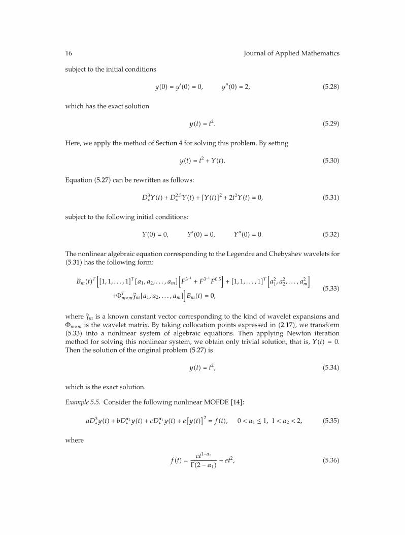
16 Journal of Applied Mathematics
subject to the initial conditions
y(0) = y′(0) = 0, y′′(0) = 2, (5.28)
which has the exact solution
y(t) = t2. (5.29)
Here, we apply the method of Section 4 for solving this problem. By setting
y(t) = t2 + Y (t). (5.30)
Equation (5.27) can be rewritten as follows:
D3∗Y (t) +D
2.5∗ Y (t) + [Y (t)]2 + 2t2Y (t) = 0, (5.31)
subject to the following initial conditions:
Y (0) = 0, Y ′(0) = 0, Y ′′(0) = 0. (5.32)
The nonlinear algebraic equation corresponding to the Legendre and Chebyshev wavelets for(5.31) has the following form:
Bm(t)T[[1, 1, . . . , 1]T [a1, a2, . . . , am]
[F3−1 + F3−1F0.5
]+ [1, 1, . . . , 1]T
[a21, a
22, . . . , a
2m
]
+ΦTm×mγm[a1, a2, . . . , am]
]Bm(t) = 0,
(5.33)
where γm is a known constant vector corresponding to the kind of wavelet expansions andΦm×m is the wavelet matrix. By taking collocation points expressed in (2.17), we transform(5.33) into a nonlinear system of algebraic equations. Then applying Newton iterationmethod for solving this nonlinear system, we obtain only trivial solution, that is, Y (t) = 0.Then the solution of the original problem (5.27) is
y(t) = t2, (5.34)
which is the exact solution.
Example 5.5. Consider the following nonlinear MOFDE [14]:
aD3∗y(t) + bD
α2∗ y(t) + cDα1∗ y(t) + e
[y(t)]2 = f(t), 0 < α1 ≤ 1, 1 < α2 < 2, (5.35)
where
f(t) =ct1−α1
Γ(2 − α1) + et2, (5.36)

Journal of Applied Mathematics 17
subject to the initial conditions
y(0) = 0, y′(0) = 1, y′′(0) = 0, (5.37)
which has the exact solution
y(t) = t. (5.38)
Here, we apply the method of Section 4 for solving this problem. By setting
y(t) = t + Y (t). (5.39)
Equation (5.35) can be rewritten as follows:
aD3∗Y (t) + bD
α2∗ Y (t) + cDα1∗ Y (t) + e[Y (t)]
2 + 2etY (t) = 0, (5.40)
subject to the initial conditions
Y (0) = 0, Y ′(0) = 0, Y ′′(0) = 0. (5.41)
The nonlinear algebraic equation corresponding to the Legendre and Chebyshev wavelets for(5.40) has the following form:
Bm(t)T[[1, 1, . . . , 1]T [a1, a2, . . . , am]
[aF3−1 + bF3−1F3−α2 + cF3−1F3−α1
]
+[1, 1, . . . , 1]T[a21, a
22, . . . , a
2m
]+ ΦT
m×mγm[a1, a2, . . . , am]]Bm(t) = 0,
(5.42)
where γm is a known constant vector corresponding to the kind of wavelet expansion andΦm×m is the wavelet matrix. By taking collocation points expressed in (2.17), we transform(5.42) into a nonlinear system of algebraic equations. By applying the Newton iterationmethod for solving this nonlinear system, we obtain only trivial solution, that is, Y (t) = 0.Then the solution of the original problem (5.35) is
y(t) = t, (5.43)
which is the exact solution.
6. Conclusion
In this paper a general formulation for the Legendre and Chebyshev wavelet operationalmatrices of fractional-order integration has been derived. Then a numerical method based onLegendre and Chebyshev wavelets expansions together with these matrices are proposedto obtain the numerical solutions of MOFDEs. In this proposed method, by a change ofvariables, the MOFDEs with nonhomogeneous conditions are transformed to the MOFDEs

18 Journal of Applied Mathematics
with homogeneous conditions. The exact solutions for some MOFDEs are obtained by ourmethod. The proposed method is very simple in implementation for both the Legendre andthe Chebyshev wavelets. As the numerical results show, the method is very efficient forthe numerical solution of MOFDEs and only a few number of wavelet expansion terms areneeded to obtain a good approximate solution for these problems.
References
[1] A. Carpinteri and F. Mainardi, Fractals and Fractional Calculus in Continuum Mechanics, Springer, NewYork, NY, USA, 1997.
[2] K. S. Miller and B. Ross, An Introduction to the Fractional Calculus and Fractional Differential Equations,John Wiley & Sons, New York, NY, USA, 1993.
[3] K. B. Oldham and J. Spanier, The Fractional Calculus, Academic Press, New York, NY, USA, 1974.[4] I. Podlubny, Fractional Differential Equations, vol. 198, Academic Press, San Diego, Calif, USA, 1999.[5] I. Podlubny, “Fractional-order systems and fractional-order controllers,” Report UEF-03-94, Slovak
Academy of Sciences, Institute of Experimental Physics, Kosice, Slovakia, 1994.[6] R. Gorenflo and F. Mainardi, “Fractional calculus: integral and differential equations of fractional
order,” in Fractals and Fractional Calculus in Continuum Mechanics, vol. 378, pp. 223–276, Springer,Vienna, Austria, 1997.
[7] W. R. Schneider and W. Wyss, “Fractional diffusion and wave equations,” Journal of MathematicalPhysics, vol. 30, no. 1, pp. 134–144, 1989.
[8] Y. Li, “Solving a nonlinear fractional differential equation using Chebyshev wavelets,” Communica-tions in Nonlinear Science and Numerical Simulation, vol. 15, no. 9, pp. 2284–2292, 2010.
[9] K. Diethelm and N. J. Ford, “Multi-order fractional differential equations and their numericalsolution,” Applied Mathematics and Computation, vol. 154, no. 3, pp. 621–640, 2004.
[10] K. Diethelm and Y. Luchko, “Numerical solution of linear multi-term initial value problems offractional order,” Journal of Computational Analysis and Applications, vol. 6, no. 3, pp. 243–263, 2004.
[11] K. Diethelm, “Multi-term fractional differential equations multi-order fractional differential systemsand their numerical solution,” Journal Europeen des Systemes Automatises, vol. 42, pp. 665–676, 2008.
[12] A. M. A. El-Sayed, A. E. M. El-Mesiry, and H. A. A. El-Saka, “Numerical solution for multi-termfractional (arbitrary) orders differential equations,” Computational & Applied Mathematics, vol. 23, no.1, pp. 33–54, 2004.
[13] A. M. A. El-Sayed, A. E. M. El-Mesiry, and H. A. A. El-Saka, “Numerical methods for multi-termfractional (arbitrary) orders differential equations,” Applied Mathematics and Computation, vol. 160,no. 3, pp. 683–699, 2005.
[14] A. M. A. El-Sayed, I. L. El-Kalla, and E. A. A. Ziada, “Analytical and numerical solutions of multi-term nonlinear fractional orders differential equations,” Applied Numerical Mathematics, vol. 60, no. 8,pp. 788–797, 2010.
[15] V. Daftardar-Gejji andH. Jafari, “Solving amulti-order fractional differential equation using Adomiandecomposition,” Applied Mathematics and Computation, vol. 189, no. 1, pp. 541–548, 2007.
[16] J. T. Edwards, N. J. Ford, and A. C. Simpson, “The numerical solution of linear multitermfractional differential equations: systems of equations,”Manchester Center for Numerical ComputationalMathematics, 2002.
[17] K. Diethelm and N. J. Ford, “Numerical solution of the Bagley-Torvik equation,” BIT. NumericalMathematics, vol. 42, no. 3, pp. 490–507, 2002.
[18] J. L. Wu, “A wavelet operational method for solving fractional partial differential equations numeri-cally,” Applied Mathematics and Computation, vol. 214, no. 1, pp. 31–40, 2009.
[19] U. Lepik, “Solving fractional integral equations by the Haar wavelet method,” Applied Mathematicsand Computation, vol. 214, no. 2, pp. 468–478, 2009.
[20] Y. Li and W. Zhao, “Haar wavelet operational matrix of fractional order integration andits applications in solving the fractional order differential equations,” Applied Mathematics andComputation, vol. 216, no. 8, pp. 2276–2285, 2010.
[21] M. U. Rehman and R. A. Khan, “The legendre wavelet method for solving fractional differentialequations,” Communication in Nonlinear Science and Numerical Simulation, vol. 227, no. 2, pp. 234–244,2009.

Journal of Applied Mathematics 19
[22] N. M. Bujurke, S. C. Shiralashetti, and C. S. Salimath, “An application of single-term Haarwavelet series in the solution of nonlinear oscillator equations,” Journal of Computational and AppliedMathematics, vol. 227, no. 2, pp. 234–244, 2009.
[23] E. Babolian, Z. Masouri, and S. Hatamzadeh-Varmazyar, “Numerical solution of nonlinear Volterra-Fredholm integro-differential equations via direct method using triangular functions,” Computers &Mathematics with Applications, vol. 58, no. 2, pp. 239–247, 2009.
[24] M. Tavassoli Kajani, A. Hadi Vencheh, andM. Ghasemi, “The Chebyshev wavelets operational matrixof integration and product operationmatrix,” International Journal of ComputerMathematics, vol. 86, no.7, pp. 1118–1125, 2009.
[25] M. H. Reihani and Z. Abadi, “Rationalized Haar functions method for solving Fredholm and Volterraintegral equations,” Journal of Computational and Applied Mathematics, vol. 200, no. 1, pp. 12–20, 2007.
[26] F. Khellat and S. A. Yousefi, “The linear Legendre mother wavelets operational matrix of integrationand its application,” Journal of the Franklin Institute, vol. 343, no. 2, pp. 181–190, 2006.
[27] M. Razzaghi and S. Yousefi, “The Legendre wavelets operational matrix of integration,” InternationalJournal of Systems Science, vol. 32, no. 4, pp. 495–502, 2001.
[28] A. Kilicman and Z. A. Al Zhour, “Kronecker operational matrices for fractional calculus and someapplications,” Applied Mathematics and Computation, vol. 187, no. 1, pp. 250–265, 2007.

Submit your manuscripts athttp://www.hindawi.com
Hindawi Publishing Corporationhttp://www.hindawi.com Volume 2014
MathematicsJournal of
Hindawi Publishing Corporationhttp://www.hindawi.com Volume 2014
Mathematical Problems in Engineering
Hindawi Publishing Corporationhttp://www.hindawi.com
Differential EquationsInternational Journal of
Volume 2014
Applied MathematicsJournal of
Hindawi Publishing Corporationhttp://www.hindawi.com Volume 2014
Probability and StatisticsHindawi Publishing Corporationhttp://www.hindawi.com Volume 2014
Journal of
Hindawi Publishing Corporationhttp://www.hindawi.com Volume 2014
Mathematical PhysicsAdvances in
Complex AnalysisJournal of
Hindawi Publishing Corporationhttp://www.hindawi.com Volume 2014
OptimizationJournal of
Hindawi Publishing Corporationhttp://www.hindawi.com Volume 2014
CombinatoricsHindawi Publishing Corporationhttp://www.hindawi.com Volume 2014
International Journal of
Hindawi Publishing Corporationhttp://www.hindawi.com Volume 2014
Operations ResearchAdvances in
Journal of
Hindawi Publishing Corporationhttp://www.hindawi.com Volume 2014
Function Spaces
Abstract and Applied AnalysisHindawi Publishing Corporationhttp://www.hindawi.com Volume 2014
International Journal of Mathematics and Mathematical Sciences
Hindawi Publishing Corporationhttp://www.hindawi.com Volume 2014
The Scientific World JournalHindawi Publishing Corporation http://www.hindawi.com Volume 2014
Hindawi Publishing Corporationhttp://www.hindawi.com Volume 2014
Algebra
Discrete Dynamics in Nature and Society
Hindawi Publishing Corporationhttp://www.hindawi.com Volume 2014
Hindawi Publishing Corporationhttp://www.hindawi.com Volume 2014
Decision SciencesAdvances in
Discrete MathematicsJournal of
Hindawi Publishing Corporationhttp://www.hindawi.com
Volume 2014 Hindawi Publishing Corporationhttp://www.hindawi.com Volume 2014
Stochastic AnalysisInternational Journal of