Embed Size (px)
Citation preview

1
A New Solution Adaption Capability for the OVERFLOW CFD Code
Pieter G. Buning NASA Langley Research Center, Hampton, VA
10th Symposium on Overset Composite Grid and Solution Technology
September 20-23, 2010, Moffett Field, CA

2
Goals
• Add a solution-adaptive grid capability for off-body (Cartesian) grids
• Make it an integral part of the OVERFLOW off-body grid generation
• Based on adaptive grid capability in OVERFLOW-D*, but able to create finer grid levels than “Level 1”
• Efficient enough for time-accurate moving grids!
* see Meakin, AIAA-95-1722 and AIAA-97-1858

3
Outline
• (Goals) • Approach • Sensor function and marking
• Grid generation and connectivity
• Interpolation onto new grid system • Sample results • Conclusions, issues, and future work

4
Approach
• Use as much of the current off-body grid generation mechanics as possible • Where we have refinement grids, either
– Blank out coarser-level grids, or
– Make all grids abutting (with added overset boundaries) • Use feature-based adaption for now
– Easier to implement than adjoint, certainly for unsteady problems – Appropriate for vortex-dominated problems like rotorcraft

5
Approach
Terminology: • Grids are either “near-body” (user-supplied) or “off-body” (Cartesian,
automatically generated) • “Level 1” off-body grids are the finest off-body grids (before
adaption), with a user-specified grid spacing • Level 2, 3, etc., are coarser by factors of 2 • Refinement grids are labelled Level -1, -2, etc., and are finer by
factors of 2 Further, • Near-body grids are always surrounded by Level 1 grids • Geometry cuts holes in Level 1 and finer off-body grids • Neighboring off-body grids differ by only one level

6
Approach
Controls: • NREFINE – maximum number of refinement levels • ETYPE – sensor function (undivided 2nd difference, vorticity,
undivided vorticity...) • EREFINE – sensor value above which we mark for refinement • ECOARSEN – sensor value below which we mark for coarsening
We would prefer to control: • Accuracy (via error estimate) • Cost (number of grid points)

7
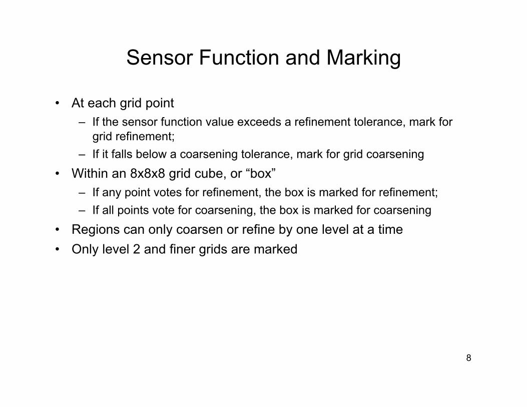
Sensor Function and Marking
• Undivided 2nd difference of (elements of) Q=(ρ, ρu, ρv, ρw, ρe0) – 2nd difference of q times Δx2; or – Difference between qi and average of (qi-1, qi+1); or – Interpolation error between current grid and 2x coarser grid; or – Truncation error estimate
• Actually computed as (normalized and squared; take max over Q variables)
• This function – Is non-dimensional – Is independent of grid units – Gets smaller as the grid is refined (where Q is smooth)
8
Sensor Function and Marking
• At each grid point – If the sensor function value exceeds a refinement tolerance, mark for
grid refinement; – If it falls below a coarsening tolerance, mark for grid coarsening
• Within an 8x8x8 grid cube, or “box” – If any point votes for refinement, the box is marked for refinement; – If all points vote for coarsening, the box is marked for coarsening
• Regions can only coarsen or refine by one level at a time • Only level 2 and finer grids are marked

9
Sensor Function and Marking
Sensor function (blue-10-10; magenta-10-3)
Marker function (blue-coarsen; green-maintain; magenta-refine)

10
Grid Generation
• Start from finest level • For each grid level (up through level 1):
1. Mark regions from previous adapt cycle refinement boxes 2. Unmark regions from current adapt cycle coarsen boxes 3. Mark regions from current adapt cycle refinement boxes 4. Mark near-body grid proximity boxes (level 1 only) 5. Mark regions from user-specified boxes
• For grid level 2 and up: 1. Fill buffer around clusters of previous-level grids 2. Clusters become rectangular 3. Merge neighboring clusters

11
Grid Connectivity
• Hole cutting – All refinement grids get cut by geometry
(just like level 1) • Blanking for refinement
– Next-finer grid level explicitly blanks out regions in current level
• Connectivity – Refinement grids can have
• Hole boundary points from geometry cuts • Hole boundary points from finer
refinement grids • Outer boundary points
Sample level (-1) grid blanking and interpolation stencils

12
Solution Interpolation onto Adapted Grids
Goals: • Process must be MPI-parallel, and include (re)load-balancing • Near-body grids (and auto splitting) do not change, so involve no
interpolation (but may move to different MPI groups) • Interpolation must be performed in-core Process: • Create new off-body grid system • Create a new distribution of near-body and off-body grids • MPI groups exchange near-body grids and solutions (no new splitting)
– This is parallelized to the extent that independent groups can exchange grids independently
• Off-body grid solution interpolation: – All MPI groups loop through old off-body grids, coarse-to-fine – Use bounding box to find which new grids touch this old grid – Owner uses non-blocking MPI sends to relevant new group(s) – New groups use blocking MPI receives, then interpolate onto new grid(s)

13
Solution Interpolation onto Adapted Grids
Original OVERFLOW-D method wrote old solutions to disk, read back in to interpolate onto new grids
+ Avoided the need for having old and new solutions in memory at the same time + Not a limitation for steady-state (adapting less than 10 times) + Not as much of a limit for “regular” problems, where less than 30% of the total grid points are in the off-body grids
– Big problem for rotorcraft problems, where more than 90% of the points are in the off-body grids, and problem is unsteady – For a sample UH-60 test case, adaption took 50% of the total time when using disk, compared to 3% when using memory

14
Sample Results – Supersonic Airfoil
• Steady flow, easy adaption • Converge first, then adapt every 10 steps for 100 steps • Nice adaption behavior, though lift chatters and residual hangs up
(even after adaption is turned off)

15
Sample Results – 2D Jet in Supersonic Cross-Flow
Sonic H2 jet (pressure ratio 100) into Mach 4 N2 free-stream • Developing shock structure and contact surface • Again, lots to adapt to • Wall grid has small normal extent, stream-wise spacing to match finest expected off-body adaption

16
Sample Results – 2D Jet in Supersonic Cross-Flow
Two different levels of refinement: • NREFINE=0 or 2 (minimum spacing of Djet/5 or Djet/20) • Results look fairly similar, but added detail with finer adaption
136 grids, 245K points 944 grids, 1269K points

17
Sample Results – Helicopter Rotor
• Coarse-grid UH-60 test case from Mark Potsdam (Army AFDD) – Main blade grid is 125x82x33 (101 points on airfoil, 33 points in surface-
normal direction, 82 span-wise stations) – Finest (level 1) off-body spacing is 20% of blade chord

18
Sample Results – Helicopter Rotor
• Adapted grid system after one revolution – Two levels of refinement – Adaption performed every 10 steps (2 deg rotation) – Much better resolution of tip vortices – Grid size increases from 5M points to 67M points

19
Sample Results – Helicopter Rotor
• Development of level (-2) grids at 90, 180, 270, 360 deg rotation

20
Sample Results – Helicopter Rotor
• Ending with 1871 grids, 67M points • Average 68 sec/step (20 sub-iterations/step), using 128 processors
– 81% flow solver – 9% idle – 6% Chimera communication – 2% overset grid connectivity – 2% grid adaption
• Breakdown of adaption process – 80% off-body solution interpolation – 15% off-body grid generation – 0.5% sensor function calculation

21
Grid Statistics
• 2D jet in supersonic cross-flow
• UH-60 rotor
Grid type # grids % points % blanked Near-body 1 5 0 Level (-2) 162 50 1 Level (-1) 86 26 10 Level 1 33 12 11 Level 2 40 6 0 … … … … total 342 100 4
Grid type # grids % points % blanked Near-body 12 3 0 Level (-2) 1153 66 2 Level (-1) 505 23 24 Level 1 79 6 28 Level 2 99 2 0 … … … … total 1871 100 9

22
Conclusions
• Solution adaption process has been implemented in OVERFLOW – Allows off-body refinement grids that are finer than Level 1 – Grid adaption is an integral part of the code – Adaption is efficient enough for time-accurate solutions – Grid blanking for refinement grids is significant but not overwhelming – Adaption process is both MPI- and OpenMP-parallel

23
Issues
• How to control the number of grid points? – Limit for run time and memory usage
• How often to adapt? – Make sure adapted region covers moving features
• Picking near-body grid resolution – Very fine means lots of points – Too coarse means we lose the benefit of adaption – We need adaption here too!

24
Issues
• Physics or numerical artifacts? – Effect of time-step and sub-
iteration count on time accuracy when refining grids

25
Future Work
• Near-body grid adaption – Needed to maintain similar resolution of features, and similar spacing in overlap
regions – One issue is maintaining smooth geometry definition
• Methods to control number of points – c.f. M.J. Aftosmis and M.J. Berger, “Multilevel Error Estimation and Adaptive h-
Refinement for Cartesian Meshes with Embedded Boundaries,” AIAA-2002-0863, Jan. 2002
• Look at other sensor functions (e.g., vorticity, adjoint, …) – c.f. S.J. Kamkar, A.M. Wissink, A. Jameson, and V. Sankaran, “Feature-Driven
Cartesian Adaptive Mesh Refinement in the Helios Code,” AIAA-2010-0171, Jan. 2010
– c.f. M. Nemec and M.J. Aftosmis, “Adjoint-Based Adaptive Mesh Refinement for Complex Geometries,” AIAA-2008-0725, Jan. 2008