Embed Size (px)
Citation preview

1
A New Seafloor Gravimeter
Glenn Sasagawa1, Wayne Crawford1,2, Ola Eiken3, Scott Nooner1 Torkjell Stenvold3,
and Mark Zumberge1
Geophysics manuscript # 01177, Accepted September 9, 2002.
Abstract: A new reservoir management application uses precise time lapse gravitymeasurements on the seafloor for the detection of seawater infiltration in offshore natural gasfields during production. Reservoir models for the North Sea Troll field predict gravitychanges as large as 0.060 mGal within a 3-5 year period. We have constructed and deployeda new instrument: the ROVDOG (Remotely Operated Vehicle deployed Deep OceanGravimeter) system for this application. Because the measurements must be accurately re-located (within 3 cm), we required a gravimeter which could be handled by an ROV andplaced atop seafloor benchmarks. We have built an instrument based around the ScintrexCG-3M land gravimeter. Motorized gimbals level the gravimeter sensor within a watertightpressure case. Precision quartz pressure gauges provide depth information. A shipboardoperator remotely controls the instrument and monitors the data. The system error budgetconsiders both instrumental and field measurement uncertainties. The instrument prototypewas deployed in the North Sea during June 1998; a total of 75 observations were made at 32stations. The standard deviation of repeated gravity measurements is 0.026 mGal; thestandard deviation of pressure derived heights, for repeated measurements, is 1.4 cm. Arefined instrument was deployed in August 2000, in a three-sensor configuration. Multiplesensors improve the precision by averaging more samples without incurring additional surveytime. A total of 159 measurements were made at 68 stations. The standard deviation ofrepeated measurements is 0.019 mGal; the standard deviation of pressure derived heights is0.78 cm. A ROVDOG pressure case rated to 4500 m depth has also been constructed. Thissystem was deployed with the manned submersible ALVIN in November 2000, to a depth of2700 m.
INTRODUCTION
In an offshore natural gas field, water slowly replaces the gas during production. The
liquid infiltration has implications for the production rates and total recoverable reserves.
Monitoring wells can observe this process but are expensive. Gravity measurements can serve
as a non-invasive, lower cost monitoring method. Water has much higher density than that of
gas and the infiltration process generates a time varying gravity signal over the gas field.
Seafloor subsidence during production, as well as the changing density distribution, also
contribute to the gravity signal. The Troll field (60º 40' N, 3º 40' E) contains an estimated 1.3
x 1012 m3 of recoverable gas reserves and is expected to be productive for decades. Models of
the water infiltration rate predicted gravity rates of change of order 0.010-0.030 mGal per
year at the sea floor. Statoil and the Troll field production partners have initiated a project to
monitor the reservoir using gravity.
1 Scripps Institution of Oceanography, University of California, San Diego, La Jolla, California 92093,USA. E-Mail: [email protected] , [email protected] , [email protected] Now at Institut de Physique du Globe de Paris, Paris, 75252, France. E-mail:[email protected] Statoil Research and Development Centre, Trondheim, NO-7005, Norway. E-mail: [email protected]

2
Gravity measurements for reservoir monitoring have been employed previously for
hydrothermal energy fields (e.g. Allis and Hunt, 1986, and San Andres and Pedersen, 1993).
Hare et al. (1999) report on the baseline gravity survey over Prudhoe Bay, in which deliberate
water injection is being used to enhance future production rates. These gravity surveys all
took place at the surface.
Seafloor gravimeter systems are commonly lowered from ships (e.g. LaCoste, 1967;
Hildebrand et al., 1990). However, precise repositioning is required for time dependent work.
Until now, no one has devised an adequate solution to this problem with sea floor gravity
surveys. A gravity survey on the seafloor has a number of advantages for providing the high
precision data required for reservoir monitoring and other geophysical studies. Stationary
seafloor measurements require no vehicle motion corrections. If used with a remotely
operated vehicle (ROV) and seafloor benchmarks, the instrument can be precisely and
repeatedly positioned. Also, a seafloor instrument is much closer to the source bodies than a
sea surface gravimeter, improving the signal-to-noise ratio. For applications involving
offshore reservoir monitoring, stationary seafloor gravimeters have the potential to collect
data of higher precision and resolution than other existing gravimeters.
Gravimeters have also been operated inside manned submersibles resting on the
seafloor (e.g. Holmes and Johnson, 1993; Cochran et al., 1994; Evans, 1996; and Ballu et al.,
1998), but vehicle motion during the measurements has been problematic. Because no
existing seafloor gravimeter system could meet all of our requirements for resolution, speed,
cost, and precise instrument relocation, we elected to build a new instrument, based around
deployment with an ROV or a manned submersible. We have also developed a methodology
for performing such surveys. This new system was named ROVDOG, for ROV deployed
Deep Ocean Gravimeter.
This paper will describe the instrument, including capabilities, performance tests and
an instrumental error budget. We will also describe our experiences in three different
seafloor surveys and compare the observed measurement repeatability with those estimated by
the error budget. We will also show that is now possible to apply this technology for offshore
reservoir monitoring applications.
INSTRUMENTATION
The ROVDOG instrument is essentially a land gravimeter modified for remote
operation on the seafloor. We extracted the gravity sensor core from a Scintrex CG-3M and
mounted it in a compact leveling mechanism. A microcontroller oversees the leveling
platform and controls data collection. Other circuitry provides power, pressure
measurements, signal conditioning, and system monitoring. The instrument assembly is
mounted in a watertight pressure case, which can be transported and deployed by a number
of different vehicles. The ROVDOG is linked to the vehicle by a flexible cable so that it can

3
be placed on the seafloor during measurements, thus decoupling it from vehicle vibrations. A
remote operator controls the instrument and can review and record the data in real time.
Multiple sensors can be deployed simultaneously on the same frame; this improves the
precision by averaging, without incurring additional survey time. Figure 1 is a cross section
view of the instrument; Table 1 lists the system specifications.
Leveling system
The CG-3M sensor resides in a double-gimbal frame driven by a pair of orthogonal
linear actuators. Each actuator has a DC motor-driven lead screw whose position is monitored
by a linear potentiometer. The actuators are controlled by the onboard microcontroller.
Once the ROVDOG sensor is deployed, the operator initiates the leveling operation. The
leveling servo first uses readings from a wide-range, low-resolution tiltmeter to coarsely level
the sensor, then it uses the CG-3M sensor's tiltmeters, which can resolve ±0.001 mrad over a
±1 mrad range. The leveling system can align the gravity sensor with the gravitational vertical
axis to within ±0.020 mrad within 30 seconds. The leveling system precision, including
calibration uncertainties, corresponds to a gravity precision of ±0.003 mGal. The range of
the leveling system is ±10° on each axis. During a measurement, the CG-3M tiltmeters are
continuously recorded in order to correct the gravity readings for instrument tilts (introduced
by the instrument settling into the seafloor sediments). The operator may also re-level the
sensor if the tilt exceeds survey criteria.
Frequency counter
The fundamental signal produced by the CG-3M gravity sensor is the electrostatic
voltage required to balance the force of gravity on the quartz spring-mass suspension. This
analog voltage (inside the temperature controlled housing) is converted by a voltage-
controlled oscillator to a pulse train whose frequency is proportional to gravity; a frequency
range of 1.5 kHz to 10 kHz corresponds to the world-wide gravity range of 7000 mGal. The
data system must measure the output frequency to 0.1 ppm to resolve a 0.001 mGal signal.
Because the standard Scintrex processing electronics are too large to fit in a small pressure
case, we developed a compact substitute. Our frequency counter obtains the required 0.1ppm
resolution in 1 second with a 20 MHz oven controlled crystal oscillator; oscillations from the
crystal are counted during an integer number of gravity signal cycles. There are no lost
cycles between samples, and the system can acquire samples at either 1 or 10 Hz.
The electronics that generate the gravity pulse train tends to drift with time, and thus
the output is periodically calibrated against an internal reference signal. A standard CG-3M
collects 12 s of gravity data followed by 1 s of calibration data, and then repeats this cycle.
During this brief calibration period the gravity signal is unsampled. As the period between
calibrations lengthens, the uncertainty from averaging uninterrupted gravity samples

4
improves but the uncertainty due to calibration drift worsens. We have characterized the
noise in each sensor's electronics and individually optimized the calibration duty cycles. In
two of the sensors, the optimum duty cycle was a 600 second interval of continuous gravity
observation followed by a 10 second calibration period. In the third sensor, the optimum was
a 130 second gravity observation interval followed by a 1 second calibration. Estimated
errors from the calibration cycles are 0.001 to 0.004 mGal.
Microcontroller
The ROVDOG is controlled by a single-board microcontroller-computer (Z-World
model BL1700). This device incorporates ten 12-bit A/D converters, 64 digital I/O lines and
four serial ports. The microcontroller software governs the leveling gimbals, monitors various
system functions, interfaces with the frequency counter and a pressure gauge, and provides
communications with a remote operator via the ROV data system. An interface board
provides power and signal distribution. Figure 2 diagrams the system signal flow.
The microcontroller, frequency counter, and interface board are mounted on top of
the gimbal frame. An input power DC-DC converter and a battery backup are also part of the
electrical subsystem. Power (20 watts on average) and a serial data link to the ROV are
provided via a 4-conductor cable to an underwater connector in the pressure case. The ROV
data system links the ROVDOG to a computer and operator aboard the support vessel. The
operator controls the instrument operation and data logging, using a graphical user interface.
Pressure gauges
The vertical position of the instrument is an essential measurement for several reasons.
First of all, the reservoir field is predicted to undergo subsidence during gas production and is
an important observable in reservoir models. Secondly, any changes in gravity must be
corrected for the contribution due to height changes, related by the free-water gradient of
order 0.223 mGal/m. For underwater applications, pressure gauges can be used to measure
the instrument depth and thus the measurement height.
The instrument depth during gravity observations is measured with a Paroscientific
quartz pressure gauge (a model 31K for depths to 700 m or a model 410K for depths to
7000 m). The gauge is housed within the ROVDOG pressure case and is coupled to seawater
through a high-pressure port. The manufacturer specifies an accuracy of 0.01% of full scale.
By averaging the results of several gauges, the precision can be improved; like the gravity
data, we require relative precision only (to obtain relative benchmark heights), and we observe
repeatability approaching 10-5 of the water depth. During a survey, seawater temperature
profiles can be collected to improve the seawater density model needed to convert pressure to
depth. However, the corrections from actual survey temperature profiles proved too small to
affect the depth accuracy.

5
Pressure case and external frame
The instrument is housed in a cylindrical watertight pressure case, which is mounted
on an external deployment frame. Currently, we have two pressure case models, rated to
depths of 700 m and 4500 m. Three of the shallow water versions can be mounted on the
same frame and still be handled by a typical ROV. A set of braces and a T-handle for ROV
manipulators completes the mechanical assembly. A four-conductor cable between the ROV
and ROVDOG provides the power and the data link. The ROVDOG power and data
requirements are supported by a number of different vehicles; little more than a cable with
the correct mating electrical connector is required for interfacing ROVDOG with a new
vehicle.
INSTRUMENT TESTS AND PERFORMANCE
After construction, a number of tests were performed to characterize the instruments.
We investigated the data system performance and its interface to the CG-3M, sensor
characteristics such as drift and tiltmeter response, and the instrument's dynamic response to
vertical acceleration. Our tests are described below.
Repeatability, drift, calibration and tilt
The repeatability, drift rate and scale factor of the CG-3M sensor were not expected to
change when installed in the ROVDOG system. The manufacturer's specified repeatability
for the CG-3M is 0.005 mGal. Eleven laboratory tests demonstrated ROVDOG repeatability
ranging between 0.003 to 0.015 mGal with a median value of 0.007 mGal. Instrument drift
(0.3-0.8 mGal/day) is routinely monitored and is consistent with the drift behavior of
unmodified CG-3M sensors (Bonvalot et al., 1998). The instrument calibration for one
instrument has been measured along our absolute gravity calibration line (Sasagawa et al.,
1989) and agrees with the manufacturer’s calibration to (8 ± 2) x 10-6. The manufacturer also
uses an absolute gravity calibration line, but with a different gravimetric range (≈948 mGal
higher). This agreement is a good indication of the linearity of the sensor.
The tilt response of the CG-3M sensor is also not expected to change, but the
ROVDOG uses an automatic leveling system. Calibration is performed by tilting the sensor
and observing the apparent gravity reading decrease as a function of the cosine of the tilt
angle. ROVDOG tilt-induced uncertainties are ±0.003 mGal. The calibration is routinely
performed before and after a survey, and also serves as a useful diagnostic test of most of the
system functions.

6
Vertical acceleration and shock
Because the Scintrex sensor was initially intended for use on land, we tested its
dynamic response to signals more typical of the seafloor environment. Seafloor seismic noise
is substantially greater than that of land sites (Collins et al., 2001). For this reason, we tested
the ROVDOG system on a seismometer vertical calibration or "shake" table. In a series of
tests, sinusoidal motions of known amplitudes and periods were applied to the ROVDOG.
Peak-to-peak amplitudes ranged up to 10 µm, and frequencies varied from 62.5 mHz (16 s
period) to 333 mHz (3 s period); these resulted in peak-to-peak acceleration signals up to 8
mGal. Control data sets with no drive signal were also collected. The difference in the mean
values between the control and the oscillating data sets in 7 trials (usually averaged for 20
minutes) ranged from -0.003 to 0.012 mGal with median value of 0.001 mGal.
Figure 3 shows an example of the power spectral density from one of these
experiments. In this one, the table oscillated with a 3 second period and a 10 µm amplitude
(two or three times larger than what can be encountered normally on the seafloor in the Troll
field). Note that while many harmonics are present in the spectrum, the noise at periods
longer than the applied signal is unaffected by the imposed oscillation.
The manufacturer's test for mechanical shocks consists of placing a block under one
of three legs of the instrument and pulling it out suddenly, causing a repeatable shock. After
collecting a control data set, we tried this with a 12.7 mm aluminum block and observed a
change of -0.014 ± 0.014 mGal. We plan to perform further tests with larger shocks,
however, as this test does not adequately reproduce the size of shock that can be encountered
in an ROV survey.
Temperature
The CG-3M fused silica spring is housed inside a temperature-controlled oven.
Because it is not possible to maintain an absolutely stable temperature, a precision thermistor
monitors temperature fluctuations of the quartz spring. The gravity values are corrected
accordingly with the manufacturer-determined coefficient (0.1316 mGal/mK for two of the
sensors and 0.1206 mGal/mK for the third). The fractional uncertainty in these values is
estimated to be no more than 0.4%. The manufacturer’s acceptable operating range is ±1
mK, but in practice the temperature fluctuations seldom exceed ±0.2 mK.
The thermal environment and insulation of the gravity sensor differs between the CG-
3M and ROVDOG. In order to determine any differences in temperature response, we placed
the instrument inside a cold vault, and the air temperature was repeatedly cycled between 14ºC
and 5ºC. The correlation between the observed gravity and ambient temperature is less than
0.001 mGal/ºC.

7
The ROVDOG CG-3M oven is powered on most of the time; one exception is during
shipment for a field survey. The oven is turned on 10 or more days prior to a measurement
(the manufacturer specifies a minimum warm-up period of 48 hours). A battery backup
system can maintain the oven temperature for up to 40 minutes, if external power is
inadvertently interrupted.
Pressure gauge calibration
The pressure gauges were calibrated against a dead-weight pressure calibrator (Ruska
model 2400-700). The gauges were placed overnight in a temperature-controlled water bath
and calibrated in situ. The scale factors provided by the vendor were in good agreement with
our calibration. However, significant offsets of order 6-10 kPa were observed. No significant
variations in the scale factor or offset were detected for a temperature range between 20° C
and 7° C.
The calibrations also show that the precision is somewhat better than that quoted by
the manufacturer. For the model 31K pressure gauges, equivalent depth precision of order 5
cm over the full range of the sensor is possible. Tests of the model 410K, to a pressure
corresponding to 2700 m, have demonstrated precision equivalent to 5 cm as well. For
surveys over a narrow depth range, the depth repeatability inferred from pressure
measurements is even better (see the next section).
SEAFLOOR MEASUREMENTS
To date, three field surveys have been conducted with the ROVDOG instruments.
Two of the surveys were in the North Sea Troll gas field, at depths averaging 300 m. The
third survey was on the Mid-Atlantic ridge, at depths of 1700 to 2700 m. Table 2 provides
additional survey details.
Seafloor benchmarks
Models predicting the gravity change over the Troll field were used to select survey
sites on the seafloor. The 1998 design consisted of 41 locations distributed over the field,
with a fairly uniform coverage having about 4 km spacing over the main gas reservoir. Six of
the stations were placed outside the field to serve as gravity reference stations, presumably
unaffected by production induced changes. A total of 49 benchmarks were deployed during
August 1997, and an additional 30 benchmarks were deployed in April 2000.
Seafloor benchmarks serve as mounting foundations to place the instruments in exact
registration on the seafloor and are an important part of accurate subsidence studies.
Seafloor benchmarks may also be more stable than those on land, due to greater temperature
stability and the lack of water table changes, since the underlying sediments and rocks are
completely saturated by seawater.

8
The benchmarks are constructed with concrete; Figure 4 presents a schematic view of
the benchmarks used (Segawa and Fujimoto [1988] have installed similar benchmarks in
sedimented areas). The cylindrical benchmark type was installed initially. The conical
benchmark type was used subsequently because of concern over disturbance from trawl
fishing. During the 2000 survey, we covered the older benchmarks with trawl protection
skirts, which are similar in shape to that of the newer benchmarks.
Based on an analysis of sediment stability (private comm., Eiliv Skomedal, 1997), we
anticipate some of the benchmarks will sink less than a few cm into the sediment during the
30 year life of the experiment. Most of the benchmark settling will occur within the first few
months after installation. The benchmark weights in water are approximately 600 kg for the
older benchmarks and 350 kg for new ones. During deployment, the ship's position was
located with a differential GPS while the benchmarks were lowered to the seafloor by a crane
and released. Short baseline acoustic navigation of the ROV usually found the benchmarks
within 5 to 10 m of their expected locations.
Shallow water operations in the North Sea
In the 1998 survey, we used a prototype system in a single gravity, triple pressure
sensor configuration; in the 2000 survey, we used the system described here in a three-sensor
configuration.
The survey procedure was straightforward. First, the vessel transited to the benchmark
location and established dynamic positioning with differential GPS. The ROV was then
launched with ROVDOG held in place by the manipulator arm and a mounting bracket. The
pilot guided the ROV to the benchmark, locating it with sonar and video cameras. The time
needed for launch, dive, and benchmark acquisition was typically 20 minutes.
Upon acquisition, the pilot maneuvered the ROV into position, placed the ROVDOG
on top of the benchmark, and released it from the manipulator. During the measurements,
the ROV sat still on the bottom 1-2 meters from the benchmark. The only link between the
sensors and the ROV during the observations was through a cable, which was weighted to lie
on the bottom, thereby mechanically decoupling the sensors from the ROV. The observer
remotely commanded the sensor to automatically level and began the measurement. Typical
observing sessions lasted 20-30 minutes, depending on the ambient noise conditions. At the
end of the session, data logging was terminated and the ROV pilot retrieved the ROVDOG
with the manipulator arm. Figure 4 illustrates the deployment process.
The ROV and instrument were recovered on deck, unless the next station was less than
2-4 km away. In that case, an underwater transit was made to the next site at 0.5-1 m/s (1-2
knots). An underwater transit over such a short distance required less time than a
recovery/launch cycle and a surface transit at 6 m/s (12 knots). During surface transits, the
instrument was kept in an ice water bath at a temperature near that of the deep water (≈7º C).

9
We made 77 observations in 5 days during the 1998 survey and 159 observations in 12 days
during the 2000 survey. Independent of the time required for benchmark deployments and
unrelated work, gravity measurements typically required 30-40 minutes at each station and 60
minutes for transits between stations.
Supporting data sets were also collected during the surveys. To aid with tide
corrections, pressure was continuously recorded with portable seafloor instruments located at
several of the benchmarks. Additional pressure measurements were also taken at the bottom
of the TROLL A production platform. Air pressure measurements were logged aboard the
survey vessel. Sea surface height observations were also made using a wave height radar on
TROLL A. Measurements of seawater density were obtained from CTD casts and CTD
measurements aboard the ROV. Gravity measurements for drift control were made on land at
the beginning and end of the surveys at an absolute gravity base station at Kollsnes, which is
45 km east of the field.
Deep water operations on the Mid-Atlantic Ridge
The 4500 m rated version of ROVDOG has been deployed in an investigation of the
extent and dip of a hypothesized detachment fault, which forms the Atlantis transform massif
at 30º 7' N, 42º 7' W (Blackman et al., 1998). Sea surface gravity measurements do not
provide the resolution needed to map the associated density contrast. We deployed a
ROVDOG instrument with the manned submersible ALVIN during November 2000. The
operation was quite similar to ROV operations, except that the operator was on board the
submersible. The survey was also limited by the submersible endurance (≈8 hours) and took
place over several days.
We occupied 17 stations along a 10 km profile over four different dives. Station
depths varied from 1760 m to 2950 m. The total gravity range was 171 mGal and observed
standard deviations of 1 s samples were markedly less than those in the North Sea surveys.
The experimental goals emphasized coverage over precision and thus only one station was
reoccupied to control drift. The drift rate calculated from the single reoccupation compared
favorably with that from control stations on land before and after the survey. The data
analysis and interpretation is currently ongoing.
DATA REDUCTION
Data files containing 1-second samples of gravity, pressure, and several instrument
parameters were created for each observation from each sensor. The normal occupation time
was 20 minutes. Noisy periods, typically encountered during leveling procedures or
biological disturbances (fish had colonized some of the seafloor benchmarks), were removed.
Corrections for tilt and instrument temperature were performed automatically. As part of the
10
quality control procedures, data subset agreement was calculated. Windowed averages of the
time series are used to generate a single gravity value for each observation.
After initial processing, we adjust the network gravity values for a best estimate of the
drift rate during the survey. We simultaneously fit for the gravity values at repeated stations
and a sensor drift rate. In the 2000 survey, the use of three sensors operating simultaneously
improved our ability to assess drift substantially. In the adjustment of the 1998 survey, we
found that the repeatability was improved by removing a single tare. Table 2 summarizes the
sampling and statistics of the three surveys.
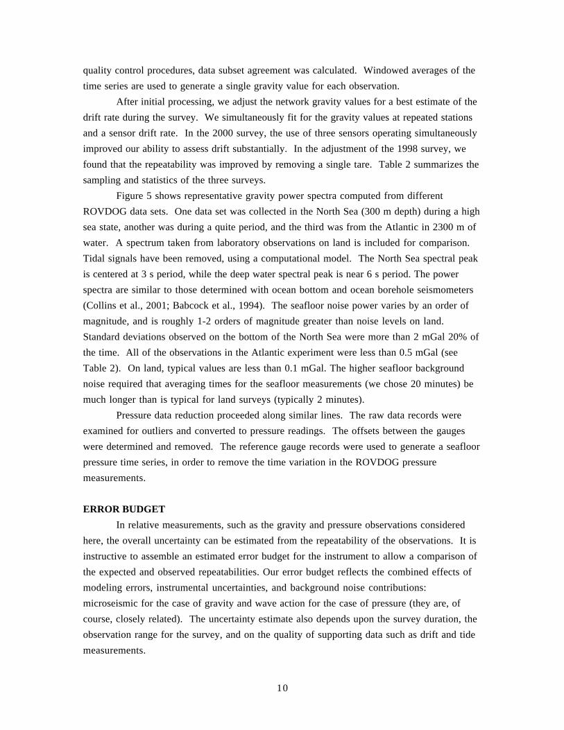
Figure 5 shows representative gravity power spectra computed from different
ROVDOG data sets. One data set was collected in the North Sea (300 m depth) during a high
sea state, another was during a quite period, and the third was from the Atlantic in 2300 m of
water. A spectrum taken from laboratory observations on land is included for comparison.
Tidal signals have been removed, using a computational model. The North Sea spectral peak
is centered at 3 s period, while the deep water spectral peak is near 6 s period. The power
spectra are similar to those determined with ocean bottom and ocean borehole seismometers
(Collins et al., 2001; Babcock et al., 1994). The seafloor noise power varies by an order of
magnitude, and is roughly 1-2 orders of magnitude greater than noise levels on land.
Standard deviations observed on the bottom of the North Sea were more than 2 mGal 20% of
the time. All of the observations in the Atlantic experiment were less than 0.5 mGal (see
Table 2). On land, typical values are less than 0.1 mGal. The higher seafloor background
noise required that averaging times for the seafloor measurements (we chose 20 minutes) be
much longer than is typical for land surveys (typically 2 minutes).
Pressure data reduction proceeded along similar lines. The raw data records were
examined for outliers and converted to pressure readings. The offsets between the gauges
were determined and removed. The reference gauge records were used to generate a seafloor
pressure time series, in order to remove the time variation in the ROVDOG pressure
measurements.
ERROR BUDGET
In relative measurements, such as the gravity and pressure observations considered
here, the overall uncertainty can be estimated from the repeatability of the observations. It is
instructive to assemble an estimated error budget for the instrument to allow a comparison of
the expected and observed repeatabilities. Our error budget reflects the combined effects of
modeling errors, instrumental uncertainties, and background noise contributions:
microseismic for the case of gravity and wave action for the case of pressure (they are, of
course, closely related). The uncertainty estimate also depends upon the survey duration, the
observation range for the survey, and on the quality of supporting data such as drift and tide
measurements.

11
The error sources for gravity and pressure are summarized in Table 3. The
”Inherent Precision” listed in each is the best possible resolution of the respective sensors.
The ”Total” uncertainty is the sum in quadrature of the inherent precision, the statistical
uncertainty, survey dependent noise terms, and modeling errors. The statistical uncertainty
incorporates background noise, and, in principle, can be reduced by longer averaging times.
To obtain representative values for the total uncertainty, we have used figures for survey
duration, survey range, and background noise levels that were typical of our surveys in the
North Sea.
Instrumental corrections
Instrumental corrections account for calibration, tilt and temperature effects. The
corrections and associated uncertainies for calibration and tilt are described in the section on
Instrument Tests and Performance. The temperature correction uncertainty for a specific
survey depends upon the precision of the temperature coefficient and the range of
temperature variations. The individual contributions are shown in Table 3.
Drift corrections
Gravimeter drift functions can be estimated through several methods. A drift
function can be fit for all repeated stations in a survey; this method samples the survey well
but is degraded by other survey noise sources. Drift functions can also be fit to repeated
observations at land base stations, which benefit from the reduced noise levels but is
infrequently sampled. Finally, the drift functions for extended observations (>24h) at
stationary land sites can be estimated, but may not be representative of the survey period.
The first method provides the best estimate of the drift function, but the variation between
different methods is a measure of the drift function uncertainty.
For a simple linear model, assume that observations take place at time t, equally
spaced from 0 to T, and that the drift rate error is Re. The drift correction errors for gravity
differences will be linear, of the form Re(t-T/2). It can be shown that the standard deviation of
the drift corrections is 12-1/2ReT
Tide correction
For both measurement types, the removal of tidal effects is important because they are
much larger than the sought after signals. For the pressure gauges, we used the records from
several recording gauges at fixed seafloor locations, allowing direct removal of the tides. The
associated uncertainty is the combined effect of noise in the reference gauges and correction
uncertainties from extrapolating the reference observations to the survey sites. Our estimates
are based on the coherence among the reference pressure gauges and their agreements with
tidal predictions.

12
For gravity we relied on a tidal prediction algorithm that models the solid earth tides
and ocean loading (Agnew, 1996) and the direct attraction of a changing water mass. The
uncertainty from tidal corrections for the gravity data is our best estimate based on our
having compared the predicted tides and observed tides at several land sites. For the seafloor
measurements, this is an area that needs further investigation.
Background noise
Both sensor types sample variations in the measured quantity once per second for the
duration of an observation (typically about 20 minutes). The uncertainty in the estimated
mean depends on the total duration and noise characteristics of the observation, which vary
with time and location. Table 3 includes a value for the statistical uncertainty that is
representative of a 20-minute observation under average noise conditions. The method of
estimating the statistical uncertainty is not simple. First, the noise spectrum is not white.
Second, for the case of the gravity sensors, the data samples are not continuous because the
sampling of gravity is interrupted every few minutes for several seconds to calibrate the
sensor's internal gravity-to-frequency conversion.
The traditional statistical uncertainty estimate is based on the assumption that the
random component of the signal is uncorrelated. However, the power spectrum of the time
series is far from flat; there is usually a fairly strong peak at about 0.3 Hz. This means the
noise process is not white, and therefore it is correlated in time. Consider the limiting case of
a periodic noise signal of period τ which averages to zero over one complete cycle. In a time
T that is not an exact integer number of cycles, the mean converges to zero as τ/T. The
standard error σ/N1/2 (typically 1 mGal / 12001/2 = 0.029 mGal) converges as T -1/2 and is an
overestimate of the statistical uncertainty in this case.
A method developed by R.L. Parker (private comm., 2000) improves on the ordinary
estimate of the mean and the standard error. The gravity time series g is convolved with a
digital filter h with the property that Σh = 1, so that constant signals are passed without
modification. If the filter is designed so that the new series h*g has a white power spectrum,
the standard theory is now applicable to it. Thus the mean and the standard deviation are
found from h*g. A suitable filter h can be obtained by taking the Fourier transform of
1/ ( )S f where S(f) is the power spectrum of the original time series. Instead of assuming
the noise is white, this approach merely requires that the signal be statistically stationary over
the period of observation. Application of this method to seafloor data reduced the standard
error estimate by a factor of 0.5 to a typical value of about 0.015 mGal
One more approach is to examine the repeatability of time-series subset averages as a
function of subset length. In doing this, we found that the uncertainty improved at a rate
between 1/N and 1/N1/2. Typically the standard deviation of the averages taken from 2-

13
minute-long subsets was below 0.01 mGal. Based on these collected analyses, we have listed
the typical contribution to uncertainty from background noise as 0.012 mGal in Table 3.
The total representative expected uncertainty for a 20 minute observation during a 12
day survey is 0.017 mGal for one gravity sensor and 0.013 kPa (1.3 cm in depth) for one
pressure sensor. The expected uncertainty of the average of three sensors is 0.010 mGal and
0.08 kPa. As can be seen in the following section, the pressure measurements met our
expectations, but the gravity measurements were less repeatable than we predicted.
SURVEY RESULTS
An important figure of merit is the measurement agreement for stations repeated
during each survey. No gravity changes are expected during the survey duration, and thus
the agreement is an estimate of the survey precision, which includes instrumental, modeling,
and acceleration noise components. The repeat station agreement also incorporates
unforeseen instrumental or survey problems. For the 1998 survey, the repeatability is 0.026
mGal; the observed repeatability for the 2000 survey is 0.019 mGal (this is the standard
deviation of the averages of three sensors). The pressure derived depth repeatability for the
1998 survey is 1.1 cm; for the 2000 survey the repeatability is 0.8 cm. Figure 6 plots the
observed agreement.
Note that the 2000 survey has improved repeatability, due to the simultaneous
measurements with multiple meters. The simultaneous data sets also allow one to detect
offsets in a single meter by a vote among all three systems. In this way, measurements with
poor agreement could be improved by rejecting at most 1/3 of the data set.
Changes in the gravity field over time provide another assessment of instrument
performance. Six stations are located outside the Troll field. The mean gravity change
between 1998 and 2000 with respect to land base station at Kollsnes is 0.002 ± 0.009 mGal.
The gravity measurements within the field are currently proprietary.
Our error budget accounts for roughly half of the observed repeatability. One
possible explanation for the 1998 repeatability is due to an electrical connector failure which
may have biased the tilt readings; the problem was not identified until after the survey.
Discussions with the manufacturer emphasized the role of shocks in degrading the
repeatability. The ROVDOG encounters greater mechanical shocks during a seafloor survey
than in a land survey. Although the sensor robustly withstands shocks of order 10 g, larger
shocks can produce gravity reading offsets. The sensor is also thought to suffer from
viscoelastic processes in the quartz suspension system, the magnitudes of which are affected
by the environment encountered between measurements (private comm., Ivo Brcic, January
2001). Such effects are difficult to detect with the infrequently repeated station
measurements in a seafloor survey. Experiments are planned to evaluate such behavior and
estimate the associated errors in the gravity readings.

14
CONCLUSIONS
Gravity measurements are useful in a number of geophysical applications, including
reservoir management and subsurface density mapping. Seafloor measurements with a
stationary, externally mounted gravimeter present a number of advantages. Compared to sea
surface gravimeters, a seafloor gravimeter is much closer to the source bodies, thus improving
the signal to noise ratio, and seafloor data requires no corrections for vehicle motion. A
seafloor gravimeter is also decoupled from vehicle vibrations. Finally, positional uncertainties
are negligible if the instrument is used with seafloor benchmarks
We have constructed, tested, and deployed a new system for precise seafloor gravity
measurement. The ROVDOG system is based upon the Scintrex CG-3M gravimeter. The
instrument can acquire a gravity time series at 1 and 10 Hz sampling rates; seawater pressure
and instrument status readings are also acquired. A number of tests have shown that the new
instrument's inherent performance is similar to that of an unmodified CG-3M; repeatability
under laboratory conditions is approximately 0.007 mGal. Multiple sensors can be deployed
simultaneously, thus improving the statistical sample size without requiring additional survey
time. The instrument is rated to depths of 700 m and 4500 m, depending upon the pressure
case used.
Actual seafloor surveys have demonstrated repeatability of 0.019 mGal with a three
sensor configuration. Simultaneous pressure measurements can resolve differences in depth
to 0.8 cm. The error budget depends upon the instrument precision and survey conditions,
such as seafloor acceleration noise and duration.
The observed repeatability is not as good as that of careful land surveys. We are
presently uncertain as to the cause of the degraded repeatability, but we suspect the primary
source is associated with the unavoidable shocks and vibrations encountered while handling
the instrument with an ROV. Additional research is being conducted to minimize these
effects, which should lead to further improvements in measurement resolution.
ACKNOWLEDGMENTS
Håvard Alnes, Valerie Ballu, and Robert L. Parker provided valuable contributions in
planning the experiment, conducting the measurements, and analyzing the data. Eric
Husmann, David Jabson, and Jacque Lemire participated in the design and fabrication of the
ROVDOG systems. The crew and pilots of the M/V Seaway Surveyor, M/V Normand Tonjer
and R/V Atlantis were crucial to the success of the program. Instrument development was
funded by Statoil and by the National Science Foundation (OCE-9819959). North Sea data
acquisition was funded by the Troll license partners: Statoil, Shell, Norsk Hydro, TotalElfFina,
and Conoco. The Mid-Atlantic expedition was funded by NSF (OCE-9712164).

15
REFERENCES
Agnew, D.C., 1997, NLOADF: a program for computing ocean-tide loading. J. Geophys.Res., 102, 5109-5110.
Allis, R.G., and Hunt, T.M., 1986, Analysis of exploitation-induced gravity changes atWairakei geothermal field, Geophysics, 51, 1647-1660.
Babcock, J. M., B. A. Kirkendall, and J. A. Orcutt, 1994, Relationships between ocean bottomnoise and the environment, Bulletin Seismo. Soc. Am., 84, 1991-2007.
Ballu, V., Dubois, J., Deplus, G.C., Diament, M., and Bonvalot, S., 1998, Crustal structure ofthe Mid-Atlantic Ridge south of the Kane fracture zone from seafloor and sea surfacegravity data, J. Geophys. Res., 103, 2615-2631.
Blackman, D.K., Cann, J.R., Janssen, B., and Smith, D.K., 1998, Origin of extensional corecomplexes: evidence from the Mid-Atlantic Ridge at Atlantis fracture zone, J. Geophys.Res., 103, 21315-21334.
Bonvalot, S., Diament, M., and Gabalda, G., 1998, Continuous gravity recording with ScintrexCG-3M meters: a promising tool for monitoring active zones, Geophys. J. Int., 135, 470-494.
Cochran, J. R., Coakley, B. J., Fornari, D. J., and Herr, R. E., 1994, Continuous underwaynear-bottom gravity measurements from a submersible, EOS, Trans. Am. Geophys. Un.,75, 579.
Collins, J.A., Vernon, F.L., Orcutt, J.A., Stephen, R.A., Peal, K.R., Wooding, F.B., Spiess, F.N.,Hildebrand, J.A., 2001, Broadband seismology in the oceans: lessons from the OceanSeismic Network Pilot Experiment, Geophys. Res. Lett., 28, 49-52.
Evans, R. L., 1996, A seafloor gravity profile across the TAG hydrothermal mound, Geophys.Res. Lett., 23, 3447-3450.
Hare, J.L., Ferguson, J.F., Aiken, C.L.V., and. Brady, J.L., 1999, The 4-D microgravitymethod for waterflood surveillance: A model study for the Prudhoe Bay reservoir, Alaska,Geophysics, 64, 78-87.
Hildebrand, J.A., Stevenson, J.M., Hammer, P.T.C., Zumberge, M.A., Parker, R.L., Fox, C.G.,and Meis, P.J., 1990, A seafloor and sea surface gravity survey of Axial Volcano, J.Geophys. Res., 95, 12751-12763.
Holmes, M.L., and Johnson, H.P., 1993, Upper crustal densities derived from sea floor gravitymeasurements; northern Juan de Fuca Ridge, Geophys. Res. Lett., 20, 1871-1874.
LaCoste, L., 1967, Measurement of gravity at sea and in the air, Rev. Geophys., 5, 477-526.
San Andres, R.B., Pedersen, J.R., 1993, Monitoring the Bulalo geothermal reservoir,Philippines, using precision gravity data, Geothermics, 22, 395-402.
Sasagawa, G.S., Zumberge, M.A., Stevenson, J.M., Lautzenhiser, T., Wirtz, J., Ander, M.E.,1989, The 1987 southeastern Alaska gravity calibration range: absolute and relativegravity, J. Geophys. Res., 94, 7661-7666.
Segawa, J., Fujimoto, H., 1988, Observation of an ocean bottom station installed in the SagamiBay and replacement of the acoustic transponder attached to it, JAMSTECTR Deep SeaResearch, 256.

16
Table 1
ROVDOG Specifications
Primary Sensors CommunicationsGravity Scintrex CG-3M Protocol RS-232Serial Numbers 9704391, 9808423, Transmission rate 9600 baud
9908435 Format ASCIIPrecision 0.005 mGal File size for 1Hz data 188 bytes/sampleRange 7000 mGal
Depth Ratings 700m and 4500mPressure ParoscientificModels 31k and 410K Dimensions 700m 4500mMaximum Rating 1000 and 10000 psi Diameter 25 cm 27 cmResolution 0.01 % of F.S. Height 57 cm 63 cm
Weight in air 25 kg 68 kgLeveling system Weight in water 2 kg 23kgPrecision ±0.020 mradLeveling Range ±10º on each axis Electrical PowerTime to level < 30 seconds Average 20W
Warm-up Peak 55 WFrequency Counter Backup time 20 minutesLeast Count 0.1 µs in 1 s Input Voltage 18-36 VDCOscillator accuracy 0.01 ppmSampling rate 10 Hz and 1 Hz
Table 1. Selected specifications for ROVDOG system. Modifications to the pressure gauge
range, input voltage range, and communications baud rate are also possible.

17
Table 2
ROVDOG Seafloor Survey Statistics and Results
June1998
August2000
November2000
Survey Duration, days 5 11 10Number of station occupations 77 159 17Number of repeated occupations 46 34 1Number of discrete stationssurveyed
38 68 17
Number of Sensors used 1 3 1σ for repeat measurements, mGal 0.027 0.021 N/Aσ for repeat pressure-derivedheights, cm
1.4 0.76 N/A
Minimum σ for 1s samples, mGal 0.6 0.4 0.1Maximum σ for 1s samples, mGal 2.8 3.8 0.5Unit 1 drift rate, mGal/day 1.196 0.893 -Unit 2 drift rate, mGal/day - 0.723 -Unit 3 drift rate, mGal/day - 0.392 0.265Support Vessel Seaway
SurveyorNormandTonjer
Atlantis
Underwater Vehicle SC-3 Hi-ROV 3000 DSV ALVIN
Table 2. A summary of performance results for three seafloor surveys with the ROVDOG
system. Standard deviation is denoted by σ.

18
Table 3
ROVDOG Error Budget – 2000 Troll Survey
1998 Survey 2000 Survey
Error Source GravityUncertainty(mGal)
PressureUncertainty(kPa)
GravityUncertainty(mGal)
PressureUncertainty(kPa)
Inherent precision 0.005 0.01 0.005 0.01Tide correction 0.003 0.22 0.003 0.10Temperature correction 0.001 0.05 0.002 0.05Drift correction 0.005 (6d) 0.05 0.010 (12d) 0.05Calibration uncertainty 0.001 0.05 0.001 0.05Tilt 0.003 0.003Background noise 0.012 0.01 0.012 0.01RMS sum 0.015 0.24 0.017 0.14Number of sensors 1 3 3 3Expected RepeatabilityFor N Sensors 0.015 0.14 0.010 0.08
Observed Repeatability 0.026 0.11 0.019 0.08
Table 3. The error budget estimate for gravity and pressure measurements, computed for the
North Sea field surveys. Expected repeatability is the quadrature sum of the terms listed.
The temperature correction uncertainty is the product of the temperature coefficient
uncertainty, the nominal temperature coefficient, and the instrument temperature variability
(±0.07 mK in 1998, ±0.35 mK in 2000) during the survey. The drift correction uncertainty
for gravity is estimated from (0.5/√3)(±0.003 mGal/day) × T, where T is the survey duration.
The calibration uncertainty for gravity is based on the scale factor uncertainty as determined
from measurements along a calibration line (±2x10⁻⁵) and the 35 mGal survey range in the
North Sea surveys. The calibration uncertainty for pressure is based on a depth range of 50
m and the manufacturer's calibration accuracy of 10-4 of full scale. Note that 0.1 kPa in
pressure corresponds to about 1 cm in depth.

19
49.5 cm
pressure case
electronics
translation stages
coarse tilt sensorshock mounts
insulation
CG-3M sensorgimbals
power supply
pressure gauge
15 degree max.rotation range
Figure 1. A cross-sectional view of a ROVDOG instrument; the 700m depth version
is shown here. The gravity sensor is taken from a Scintrex CG-3M land meter. Power
and data are provided through an umbilical cable (not shown). Mechanical
manipulators can grip the T-handle at the top of the instrument.

20
ScintrexCG-3MSensorCore Leveling
Motor
Coarse Tilt
Fine Tilt
Add
ition
alSe
nsor
s
Micro-Controller
Pressure Gauge
500 m Tether
ship-basedPC
10 mUmbilical
(Com,Power)
ROVDOG�(1 of 3)
ROV
FrequencyCounter
MotorDrivers
Com 1A/D
Digital I/OCom 2
Figure 2. A signal flow diagram of the ROVDOG system. The micro-controller
executes the detailed operation of the instrument, and exchanges pre-processed data
and commands with the operator. The operator uses a graphical user interface
(LABVIEW) to operate the instrument remotely and to view and log the data.

21
10-1
100
10-4
10-2
100
102
Frequency (Hz)
Pow
er s
pect
ral d
ensi
ty (
mG
al2 /H
z) shake table on shake table off
Figure 3
Figure 3. The power spectral density is shown for two times series. Each is derived
from the gravity sensor output sampled 10 times per second for about 15 minutes.
During one of the experiments, the sensor was on a seismometer calibration table
oscillating vertically with a 10 micron amplitude and 3 s period.

22
���������������������
1 meter
Figure 4. A sketch illustrating a ROVDOG deployment on the seafloor. The two
types of benchmarks used in the TROLL field survey are shown. The ROV,
ROVDOG, and the benchmarks are all shown in the same relative scale.

23
10−2
10−1
100
10−3
10−2
10−1
100
101
Gravity Power Spectral Density
Hz
mG
al2 /H
zTrollHigh Swell
TrollLow Swell
MAR2300m Depth
On Land
Figure 5. Power spectral density comparison for three seafloor sites and a land site. The
Troll spectra were collected at depths of 300 m on sediment, while the MAR (Mid-Atlantic
Ridge) spectra was collected on rock covered with calcium carbonate deposits. Significant
wave heights of 3-3.5 m were observed during the high swell state; wave heights of 0.5-1 m
were observed during the low swell state. The seafloor time series are approximately 20
minutes long with 1 second sample intervals; the frequency bin interval is 15.6 mHz. The
land spectra was collected in our coastal laboratory; the record is 21 hours long and the
frequency bin interval is 2 mHz.

24
0
1
2
3
4
5
6
7
8
9
10
11
-0.04 0.04-0.02-0.03-0.05 -0.01 0.01 0.02 0.03 0.050.00
Deviation from station mean (mGal)
Cou
nt
Figure 6a. Repeatability of gravity measurements for the August 2000 survey. Plotted is the
deviation from station means for 34 repeated sites over 14 stations. The standard deviation is
0.019 mGal.
6
4
2
0
8
10
12
0.00-0.50-1.00-1.50 0.50 1.00 1.50
Deviation from station mean (cm)
Cou
nt
Figure 6b. Repeatability of depth measurements derived from pressure for the August 2000
survey. Plotted is the histogram of station means for 53 repeated sites over 19 stations. The
standard deviation is 0.8 cm.