A new numerical approach for simulation of pattern ... · A new numerical approach for simulation of pattern formation models on stationary and growing surfaces ... 1 0 @ z 1 z 2

A new numerical approach for simulation ofpattern formation models on stationary and

growing surfaces

Mahdieh SattariJukka Tuomela

November 4, 2013

Outline

Motivation

Schnakenberg model

Triangulation and implementation

Examples on growing manifolds

Role of eigenfunction in pattern evolution

Conclusion

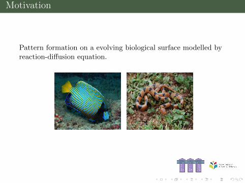
Motivation

Pattern formation on a evolving biological surface modelled byreaction-diffusion equation.

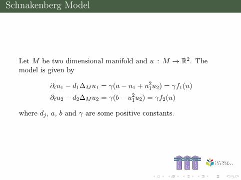
Schnakenberg Model

Let M be two dimensional manifold and u : M → R2. Themodel is given by

∂tu1 − d1∆Mu1 = γ(a− u1 + u21u2) = γf1(u)

∂tu2 − d2∆Mu2 = γ(b− u21u2) = γf2(u)

where dj , a, b and γ are some positive constants.

Schnakenberg Model

The stationary problem

− d1∆Mu1 = γ(a− u1 + u21u2)

− d2∆Mu2 = γ(b− u21u2)

The constant (positive) solution is

u =(a+ b,

b

(a+ b)2

)

Schnakenberg Model

To get diffusion-driven instability, choose a and b such that

(a+ b)3 + a− b > 0 and a < b

Schnakenberg Model

and diffusion parameters such that√d2d1

>(a+ b)

(a+ b+

√2b(a+ b)

)b− a

In particular d2 > d1.

Variational formulation

To solve model on the sphere S2 with metric g, let Vh be somefinite dimensional subspace of H1(S2) and let

Vh = span(ψ1, . . . , ψm

)The approximate solution u = (u1, u2) can be written as

uj(x, t) =

m∑i=1

cji (t)ψi(x)

Variational formulation

Find (u1, u2) such that

∂t

∫S2

u1ψjωS2 + d1

∫S2

g(grad(u1), grad(ψj))ωS2 = γ

∫S2

f1(u)ψjωS2

∂t

∫S2

u2ψjωS2 + d2

∫S2

g(grad(u2), grad(ψj))ωS2 = γ

∫S2

f2(u)ψjωS2

where ωS2 is the area form.

Discretization

Let δt be the time step and cj,ni = cji (nδt) and

unj =

m∑i=1

cj,ni ψi ≈ uj(x, nδt)

using implicit Euler method for time discretization((1 + δt γ)Mn+1 + δt d1R

n+1 − δt γ Mn)c1,n+1 = Mnc1,n + δt γ aFn+1(

Mn+1 + δt d2Rn+1 + δt γ Mn

)c2,n+1 = Mnc2,n + δt γ bFn+1

Discretization

where

Mnij =

∫S2

ψiψjωnS2 Rnij =

∫S2

g(grad(ψi), grad(ψj))ωnS2

Enijk` =

∫S2

ψiψjψkψ`ωnS2 Fni =

∫S2

ψiωnS2

Mnij =

∑k,`

En+1ijk` c

1,nk c2,n` Mn

ij =∑k,`

En+1ijk` c

1,nk c1,n`

Domain composition

The sphere S2 is covered with 6 patches Dj

D1 = (−1, 1)× (−1, 1) ϕ1(z) = γ− 1

21

z1z21

D2 = (1, 3)× (−1, 1) ϕ2(z) = γ

− 12

2

1z2

2− z1

D3 = (−1, 1)× (1, 3) ϕ3(z) = γ

− 12

3

z11

2− z2

Dj+3 = Dj ϕj+3 = −ϕj

where

γ1 = 1+|z|2 , γ2 = 1+(z1−2)2+z22 , γ3 = 1+z21+(z2−2)2

Hence ϕj : Dj → S2

Identification

Identification

Triangulation

Using Riemannian metric Gj = dϕTj dϕj in triangulation

Triangulation

Changing manifold

The growing manifold is topologically the sphere S2 withchanging Riemannian metric.To produce the growing manifold, define β : S2 → R3 andϕj = β ◦ ϕj then the Riemannian metric is

Gj = dϕTj dϕj = dϕTj dβTdβdϕj

Growing sphere (Isotropic grow)

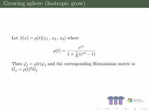
Let β(x) = ρ(t)(x1 , x2 , x3) where

ρ(t) =ert

1 + 1K (ert − 1)

Then ϕj = ρ(t)ϕj and the corresponding Riemannian metric isGj = ρ(t)2Gj


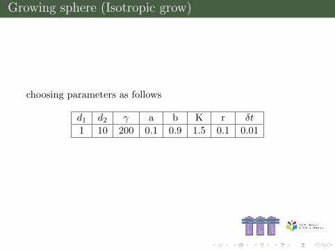
choosing parameters as follows

d1 d2 γ a b K r δt

1 10 200 0.1 0.9 1.5 0.1 0.01


The concentrations u1 and u2 at t = 5







Evolving sphere (Anisotropic grow)

Defineβ(x) =

(lx1 , lx2 , (lx3/h)1/2p

)such that

h(t) = l(t)q(t)2p

q(t) = q0β+(1−β)e−rt

l(t) = l0(1 + α(1− e−kt)

)


Choose parameters as

d1 d2 γ a b q0 l0 α β r k p

1 100 500 0.1 0.9 0.5 0.1 0.8 0.3 0.5 0.5 5



The concentrations u1 and u2 at t = 0.1 with δt = 0.0005







Eigenfunctions role in pattern formation

y1 and y2 are two positive roots of

p0(y) = d1d2(a+ b)y2 +(

(a+ b)3d1 + (a− b)d2)y + (a+ b)3

Then we call I = (y1, y2) critical interval.Let λ be an eigenvalue of −∆ and vλ be the correspondingeigenfunction.If λ/γ ∈ (y1, y2) then the linearized Schnackenberg problem hasa solution of form Cvλe

µγt where µ is the positive solution of

p1(µ, λ) = (a+b)µ2+(

(d1+d2)(a+b)λ+(a+b)3+a−b)µ+p0(λ)

Eigenfunction and pattern formation

Choosing parameters as follows

d1 d2 a b

1 10 0.1 0.9

The computed critical interval is I = [0.2, 0.5].


Let t = 1.6 be the ending time.

λ1 = 3.64 and λ2 = 14.76 are two first eigenvalues.

Set γ = 15 then just λ1/γ ∈ I = [0.2, 0.5].


The eigenfunction and concentration u1


Changing the parameter as follows

d1 d2 a b

1 20 0.2 1

The computed critical interval is I = [0.169, 0.425].


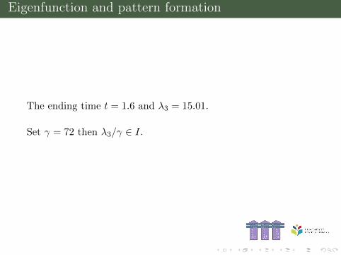
The ending time t = 1.6 and λ3 = 15.01.

Set γ = 72 then λ3/γ ∈ I.


The eigenfunction and concentration u1

Our approach can also readily be extended to morecomplicated surfaces.

Since all computations are done in two dimensionaldomains there is no error related to the approximation ofthe surface in three dimensional space.

In the case of restricting the parameters such that oneeigenvalue of Laplace operator belongs to the criticalinterval, we are able to predict sort of pattern formation.

The method benefits from simplicity in programming fordifferent kinds of curved surfaces.

Question?

Thanks for your attention

Documents

A new numerical approach for simulation of pattern ... · A new numerical approach for simulation of pattern formation models on stationary and growing surfaces ... 1 0 @ z 1 z 2