Vol.:(0123456789)1 3

GPS Solutions (2021) 25:71 https://doi.org/10.1007/s10291-021-01109-y

ORIGINAL ARTICLE

A new method to estimate GPS satellite and receiver differential code biases using a network of LEO satellites

Liangliang Yuan1,2,3  · Mainul Hoque1 · Shuanggen Jin2,3,4

Received: 8 November 2020 / Accepted: 17 February 2021 / Published online: 9 March 2021 © The Author(s) 2021

AbstractThe differential code biases (DCBs) of the global positioning system (GPS) receiver onboard low-Earth orbit (LEO) satel-lites are commonly estimated by a local spherical symmetry assumption together with the known GPS satellite DCBs from ground-based observations. Nowadays, more and more LEO satellites are equipped with GPS receivers for precise orbit determination, which provides a unique chance to estimate both satellite and receiver DCBs without any ground data. A new method to estimate the GPS satellite and receiver DCBs using a network of LEO receivers is proposed. A multi-layer mapping function (MF) is used to combine multi-LEO satellite data at varying orbit heights. First, model simulations are conducted to compare the vertical total electron content (VTEC) derived from the multi-layer MF and the reference VTEC obtained from the empirical ionosphere model International Reference Ionosphere and Global Core Plasmasphere Model. Second, GPS data are collected from five LEO missions, including ten receivers used to estimate both the satellite and receiver DCBs simultaneously with the multi-layer MF. The results show that the GPS satellite DCB solutions obtained from space-based data are consistent with ground-based solutions provided by the Centre for Orbit Determination in Europe. The proposed normalization procedure combining topside observations from different LEO missions has the potential to improve the accuracies of satellite DCBs of Global Navigation Satellite Systems as well as the receiver DCBs onboard LEO satellites, although the number of LEO missions and spatial–temporal coverage of topside observations are limited.

Keywords Global positioning system (GPS) · Differential code bias (DCB) · Normalization method · Mapping function (MF)

Introduction

Dual-frequency GNSS observations are commonly used to estimate ionospheric total electron content (TEC) as well as satellite and receiver differential code biases (DCBs), while the estimations of TECs and DCBs are closely correlated (Mannucci et al. 1998). When estimating the

satellite and receiver DCB, one of the significant error sources is the mapping error, which affects the accuracy of the vertical TEC (VTEC) parameterization, while the VTEC parameterization is also crucial in DCB estima-tions. The mapping function (MF) has been widely used to convert slant TEC to vertical TEC, such as the cosine MF and F&K MF (Foelsche and Kirchengast 2002). Many studies and evaluations have been conducted on these two MFs (Huang and Yuan 2013; Xiang and Gao 2019; Zhong et al. 2016a). The MF plays a significant role in iono-spheric VTEC modelling and DCB estimations due to the fact that the accuracy of the MF is highly correlated with the estimated VTEC and DCB. The factor that signifi-cantly impacts the accuracy in the single-layer MF is the effective ionospheric height. Lanyi and Roth (1988) found that the effective ionospheric height was between 350 and 400 km around the peak ionization height. Brunini (2011) investigated the impact of the effective height between 300 and 550 km on VTEC and DCB estimations. Three

* Shuanggen Jin sgjin@shao.ac.cn; sg.jin@yahoo.com

1 Institute of Solar-Terrestrial Physics, German Aerospace Center, Kalkhorstweg 53, 17235 Neustrelitz, Germany

2 University of Chinese Academy of Sciences, Beijing 100049, China

3 Shanghai Astronomical Observatory, Chinese Academy of Sciences, Shanghai 200030, China

4 School of Remote Sensing and Geomatics Engineering, Nanjing University of Information Science and Technology, Nanjing 210044, China

GPS Solutions (2021) 25:71

1 3

71 Page 2 of 12

different MFs, namely lear MF, cosine MF and F&K MF, were evaluated, and the effective height was analysed by Zhong et al. (2016a). For the simplicity of the ionospheric VTEC modelling, the effective height is usually fixed. For example, the effective height is set as 350 km in a wide area augmentation system like SBAS as 450 km in the global ionospheric maps (GIMs) provided by the Centre for Orbit Determination in Europe (CODE) (Lanyi and Roth 1988; Schaer et al. 1998; Hernández-Pajares et al. 2009). However, since the Earth’s ionosphere is not spheri-cally symmetric, the effective height varies with the func-tion of location, time and solar activity. Therefore, a vary-ing ionospheric height was used instead of a fixed height to reduce the mapping errors (Xiang and Gao 2019).

Various methods based on the single-layer MF were proposed in the past decade. For example, a zero method was proposed and tested using long-term CHAMP and GRACE observations by Zhong et al. (2016b). GPS P1-P2 DCBs and VTEC above JASON-2 orbit height were esti-mated with JASON-2 POD observations epoch by epoch by Wautelet et al. (2017). Li et al. (2017) estimated the GPS and BDS satellites DCB as well as receiver DCB onboard FY-3C using the same method as Wautelet. Lin et al. (2016) proposed an approach to estimate the GPS satellite DCB based on the ionospheric spherical sym-metry assumption for Challenging Minisatellite Payload (CHAMP) and Constellation Observing System for Mete-orology, Ionosphere, and Climate (COSMIC) observations. It was found that the GPS satellite DCB estimates based on CHAMP were much better than those based on COSMIC. Yuan et al. (2020) proposed an inequality constrained least squares method to estimate the COSMIC receiver DCBs. However, previous works mentioned above were based on one individual LEO mission and ionospheric single-layer assumption.

With the increasing number of LEO satellites, the advantage of combining multi-LEO observations needs to be realized. For example, we propose a new method to estimate the LEO receiver DCB as well as GPS sat-ellite DCB simultaneously for the first time by combin-ing topside observations from different LEO missions at different orbit heights with the multi-layer MF instead of single-layer MF. In addition, the performance of the multi-layer MF is evaluated through model simulations using the International Reference Ionosphere (IRI) (Blitza 2001) and Global Core Plasmasphere Model (GCPM) (Gallagher et al. 2000) and compared with the single-layer MF. The proposed normalization method is then described in detail. The evaluation of the proposed method and comparisons among different methods are presented later. Finally, the major findings are summarized, and discussions of the proposed method are reviewed along with some future challenges.

Mapping function evaluations

As is mentioned in the introductory section, the single-layer assumption is commonly used in the DCB estimation. In this section, two kinds of MFs, namely the F&K geometric MF and multi-layer MF, will be introduced. And the advantages and disadvantages of each MF are discussed through model simulation.

Single‑layer model

In the single-layer model (SLM), it is usually assumed that the ionospheric electrons are concentrated on a spherical shell of infinitesimal thickness at a fixed ionospheric effective height surrounding the Earth (Spilker 1991). For the cosine MF, the thickness of this single layer is assumed to be infinitesimal, which means all electrons are located in the position of the ionospheric pierce point (IPP). For the geometric MF, the thickness is assumed to be the altitude difference between the effective height and the receiver height, which means all elec-trons homogeneously lie in this belt. The ratio of the slant path through the pierce point and corresponding vertical path in this belt can be calculated as follows

where θ is the elevation angle, Re is the mean radius of the Earth, hLEO is the altitude of the LEO orbit and hion is the altitude of the ionospheric single layer.

Multi‑layer MF

In the multi-layer MF, the MF or obliquity factor is computed for each LEO-GPS ray path using Global Ionosphere Maps (GIM) and multi-layer ionosphere assumption. Since GIMs provide two-dimensional TEC maps, the common practice is to use the single-layer MF for vertical to slant conversions. Instead of collapsing the vertical structure of the ionosphere into a thin or thick shell, we consider that the ionosphere is composed of numerous thin shells between which the vertical structure is modeled by a Chapman profile (Garriott and Rish-beth 1969) and a superposed exponential decay function for describing the topside ionosphere and plasmasphere (Jakowski et al. 2002). Thus, the ionospheric and plasmaspheric electron densities are NI

e(h) and NP

e(h) modeled as a function of height

h by

(1)

�MFF&K =

sin �+√R−2−cos2�

1+R−1

R =�Re + hLEO

�∕�Re + hion

�

(2)Ne = NIe(h) + Np

e(h)

GPS Solutions (2021) 25:71

1 3

Page 3 of 12 71

where Nm is the peak electron density observed at the alti-tude hm , z = (h − hm)∕H and H is the atmospheric scale height. The quantity np is the plasmaspheric basic density of electrons and Hp is the mean scale height of the plasma den-sity. Note that the plasmaspheric profile NP

e below the elec-

tron density peak height hm is set as 0. Based on a simulation study, the values of np and Hp are optimized as Nm/250 and 4000 km for COSMIC and Polar Orbiting Meteorological Satellites (MetOp) satellites, and Nm/90 and 10,000 km for Gravity Recovery and Climate Experiment (GRACE) and TerraSAR-X satellites. These two parameters are listed in Table 1 as a function of the receiver height, and we can fur-ther derive np and Hp for any receiver height through inter-polation. In the multi-layer approach, the MF is defined by

where STECmodel is the slant TEC along the LEO-GPS path and VTECmodel is the corresponding VTEC. The VTEC is defined as the VTEC from the LEO orbit height up to the GPS orbit height for which the measurement point is con-sidered at the intersection point between the slant path and the effective height layer. Based on GCPM and IRI model simulations, the effective height is defined as 1400 km for COSMIC and METOP satellites and 1000 km for GRACE and TerraSAR-X satellites (Zhong et al. 2016a).

Since the ionosphere is considered to be composed of numerous thin shells, a slant path intersects each ionospheric shell characterized by shell heights of h1… hi (see right plot of Fig. 1 for illustration). The intersection points are projected

(3)

⎧⎪⎨⎪⎩

NIe(h) = Nm exp

�1

2(1 − z − exp (−z))

�

NPe(h) = np exp

�−

h

Hp

�

(4)MFmultilayer =STECmodel

VTECmodel

onto a 2D thin-shell surface, which in our case is 450 km (Mannucci et al. 1998), where corresponding VTECs are com-puted from a TEC map as VTECIPP1, VTECIPP2 … VTECIPPi. The incremental STEC, namely ΔSTEC1, ΔSTEC2 … ΔSTECi, can be computed along the ray path by multiplying the VTECIPP1, VTECIPP2 … VTECIPPi with the corresponding obliquity factors. For a Chapman layer, the obliquity factor Fi can be determined by (Hoque and Jakowski 2013)

(5)

Fi

�hi, �

�≈

1�1 −

�(hi+Re) cos (�i)

hmIPPi+Re

�2

⎡⎢⎢⎢⎣erf

⎛⎜⎜⎜⎝−exp

�−

hi−hmIPPi

HmIPPi

�√2

⎞⎟⎟⎟⎠

⎤⎥⎥⎥⎦

hi+1

hi

Table 1 Two parameters in (3), i.e. Nm∕np and Hp as a function of receiver height

ParameterReceiver height (km)

Nm∕np Hp(km)

0 125 10,000100 125 10,000200 125 10,000300 60 10,000400 60 10,000500 90 10,000600 150 8000700 200 6000800 250 4000900 250 30001000 300 2500

Fig. 1 Schematics of F&K MF (top) and multi-layer MF (bottom)

GPS Solutions (2021) 25:71

1 3

71 Page 4 of 12

where erf is the error function (Yuan et al. 2020), hi and hi+1 are the lower and upper shell heights of the ith layer along the ray path, respectively, and �i is the elevation angle at the lower shell height, hmi is the peak ionization height, Hi is the atmospheric scale height and Re is the Earth mean radius. The obliquity factor for the plasmaspheric layer can be determined by numerical integration.

Alternatively, ΔSTEC1, ΔSTEC2 … ΔSTECi can be computed along the ray path by multiplying the corre-sponding electron densities Ne1, Ne2 … Nei by the length of each segment (right panel of Fig. 1). Equations (2) and (3) indicate that the electron densities can be derived if Chapman layer parameters such as the peak ionization Nm1, Nm2, … Nmi, peak height hm1, hm2, … hmi, atmospheric scale height H1, H2, … Hi and plasmaspheric basic densities np1, np2, … npi are known. The Chapman layer approximation VTEC = 4.13HNm (Hoque and Jakowski 2007) is used for computing Nmi using VTECIPPi for fixed Hi = 70 km. The hmi (= 350 km) and Hi are kept constant for simplicity. Empiri-cal model values can be used as an alternative. The plas-maspheric basic density npi is determined dividing Nmi by a predefined factor as mentioned earlier. Finally, STEC (black bold line, right plot, Fig. 1) is computed by summing all the ΔSTEC values and represented by STECmodel in (4). Simi-larly, VTECmodel (blue broken line, right plot, Fig. 1) in (4) is computed by summing all the ΔVTEC values. The reference location of the VTEC is identified as the intersection point of the slant path and the effective height layer. As shown in Fig. 1, we used only one projected VTEC for the VTECmodel computation, namely VTECIPP2, and derived the correspond-ing Nm and np. This means that a single Chapman profile and a single plasmasphere profile are used for the VTECmodel computation between LEO and GNSS orbits. Thus, when both STECmodel and VTECmodel are computed, MFmulti-layer is finally computed by (4).

Comparison of MFs

To evaluate the performance of the multi-layer MF on the VTEC conversion, we conduct a model simulation using IRI for the ionospheric part and GCPM for the plasmaspheric part. To take different possible mapping cases into account, the simulations are conducted over the whole globe with an interval of 2.5° in both latitude and longitude and for all azi-muth angles with an interval of 6°. Here we divide the whole ionosphere into 57 layers, of which the 38 lower layers are divided by an interval of 50 km and the 19 upper layers are divided from approximately 2000 km to the GPS height by an interval of 1000 km. As it is different from the geometric mapping function, the multi-layer mapping function needs some apriori information, such as the global ionospheric map (GIM). The STEC and VTEC are obtained by integrat-ing the electron densities along each ray and neglecting the

bending effect. Furthermore, the global VTEC map calcu-lated directly from the empirical model in the simulation plays the same role as GIM does in the practical application of the multi-layer MF.

We choose March 2013 as the testing period when the F10.7 is approximately 130 sfu (solar flux unit) which rep-resents a medium solar activity. For convenience, here we adopt the optimal effective heights for the geometric MF derived through the integral and centroid definitions using the same model, i.e. GCPM, from Zhong et al. (2016a), which is expressed as follows

where hcentroid is the centroid definition of the effective height, hintegral is the integral definition of the effective height and hLEO is the orbit altitude of the LEO satellite. Since the integral effective height is not well defined for receivers at low heights, the effective ionospheric height for the receivers at the height of 0 km is kept constant as 450 km. For con-venience, the parameters such as peak ionization height hmi and atmospheric scale height Hi are kept constant as 350 km and 70 km, respectively, in the MF evaluations, since it is not convenient to calculate the peak ionization height or scale height for all simulation events from the electron density profile given by the empirical model. In practical applica-tions presented later in Sect. 3, results could be improved by knowing their actual values, for example, from supplemen-tary measurements. Alternatively, the peak height hm can be derived from the Neustrelitz Peak Height Model (Hoque and Jakowski 2012) and scale height H can be derived from NTCM (Jakowski et al. 2011) together with the Neustrelitz Peak Density Model (Hoque and Jakowski 2011) via slab thickness estimation and Chapman layer assumption.

Figures 2 and 3 show the comparison of mapping errors with respect to the receiver heights and elevation angles. The relative VTEC error with respect to the model value is defined as

where VTECactual is the actual model value and VTECmapping is the projected value from slant TEC values based on MFs. It can be seen that in case of integral definition of the effec-tive heights, the performance of the multi-layer MF is con-siderably better than the F&K MF. Mapping errors from the multi-layer MF for almost all elevation angles are less than 5%, while those from the F&K MF are varying from 5 to 15% depending on the elevation angles. In case of cen-troid definition of the effective heights, the performance of the multi-layer MF is significantly better than the F&K MF for receivers at the heights of 0 and 200 km, while the performances of these two MFs are comparable and both

(6){

hcentroid = 2.18hLEO + 571

hintegral = 1.84hLEO − 14

(7)Errorrel =(VTECactual − VTECmapping

)∕VTECactual

GPS Solutions (2021) 25:71

1 3

Page 5 of 12 71

excellent (less than 5%) for receivers higher than 500 km. In order to better understand the differences between the F&K MF and multi-layer MF, the VTEC conversion error distributions for receivers at the height of 500 km based on both MFs are presented in Figs. 4 and 5. The dashed lines represent the median value of corresponding error distri-butions. It can be seen in Fig. 4 that there is a positive or right offset away from the origin in the histogram of relative mapping errors for the F&K MF and integral definition of the effective heights, which means that the F&K MF overall underestimates the VTEC due to the ionospheric horizontal gradient effect in the model. Compared with the F&K MF, the histogram of the multi-layer MF has no such distinct shift, which implies that the multi-layer MF can reduce the horizontal gradient effect by taking horizontal ionospheric

electron density structure into account. By comparing map-ping errors using different effective heights for the F&K MF, the performance of the F&K MF using centroid definition of the effective heights is much better than that using integral definition of the effective heights for space-based receivers, which is consistent with conclusions derived by Zhong et al. (2016a). It is crucial to remember that the optimal effec-tive height used in this model simulation is derived directly from the model IRI and GCPM. Thus, the performance of

Fig. 2 Comparisons of mapping errors (absolute value of the medians of relative VTEC errors with respect to the model values) between two mapping functions, i.e. F&K and multi-layer mapping functions, using integral definition of the effective heights for a receiver at dif-ferent heights, i.e. a 0 km; b 200 km; c 500 km; d 800 km

Fig. 3 Comparisons of mapping errors (absolute value of the medians of relative VTEC errors with respect to the model values) between two mapping functions, i.e. F&K and multi-layer mapping functions, using centroid definition of the effective heights for a receiver at dif-ferent heights, i.e. a 0 km; b 200 km; c 500 km; d 800 km

Fig. 4 Histograms of relative VTEC mapping errors for different elevation angles using integral effective heights for receivers at the height of 500 km. Note that the relative VTEC errors are calculated as (VTECactual − VTECmapping

)∕VTECactual

Fig. 5 Histograms of relative VTEC mapping errors for different elevation angles using centroid effective heights for receivers at the height of 500 km

GPS Solutions (2021) 25:71

1 3

71 Page 6 of 12

the F&K MF shown in this section can be regarded as the best performance for both effective height cases. As men-tioned above, the multi-layer MF is capable of considering the ionospheric horizontal electron gradient effects by mak-ing use of the background VTEC map. The introduction of ionospheric electron profiles is supposed to be beneficial to reduce the effects of uncertainties of effective ionospheric heights. In other words, if the ionospheric effective height changes to some extent, for instance, by increasing several hundreds of kilometres, the multi-layer MF performances will change much more slightly than the F&K MF, which can be shown in Figs. 2 and 3. Thus, an apparent and valid advantage of the multi-layer MF is that the performance of the multi-layer MF does not strongly depend on the choice of the effective ionospheric height while the change of effective ionospheric height will definitely result in a VTEC conver-sion bias in geometric mapping functions. In practice, the performance of the F&K MF is very likely to degrade due to the lack of information on the optimal ionospheric effective height. On the other hand, the scale height and peak elec-tron density height are kept constant for convenience, which may degrade the performance of the multi-layer MF in the model simulation compared with that in practical applica-tions. These two facts may enhance the advantage of the multi-layer MF in GNSS applications.

Data and methodology

In this section, a new VTEC normalization approach is proposed to estimate the GPS satellites DCB and GNSS receiver DCB onboard LEO combining different LEO mis-sions, including GRACE (Tapley et al. 2004), COSMIC (Anthes et al. 2008), TerraSAR-X (Yoon et al. 2009) and MetOp A/B (Bartalis et al. 2007). One of the motivations of this work is that the LEO constellations cannot cover the global ionosphere in an inertial reference frame. With the help of the multi-layer MF, the topside observations pro-vided by different LEO missions can be normalized to the same altitude so that the coverage of the topside observa-tions is broadened significantly. The other motivation is that the number of available GPS satellites in view for one LEO satellite is limited at any one moment. When estimating GPS transmitter DCB using only LEO topside observations from one mission, the lack of some observable GPS satellites in view may lead to difficulty in applying the zero-mean con-dition for the whole GPS constellation (Zhong et al. 2015; Wautelet et al. 2017). We therefore propose combining more available LEO satellites at different orbit heights. For exam-ple, we can establish a VTEC map above 800 km (approxi-mately COSMIC orbit height) up to GPS height combining all these five LEO missions by normalizing all the topside observations to 800 km. The LEO receiver DCB and GPS

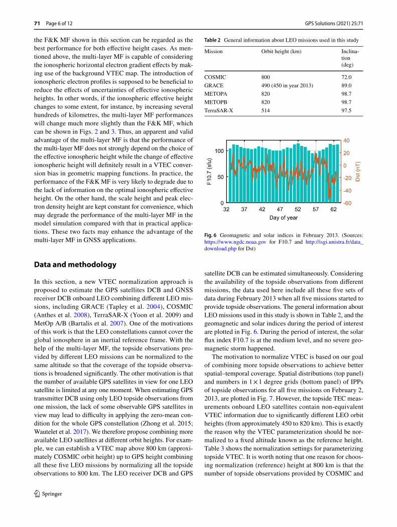
satellite DCB can be estimated simultaneously. Considering the availability of the topside observations from different missions, the data used here include all these five sets of data during February 2013 when all five missions started to provide topside observations. The general information about LEO missions used in this study is shown in Table 2, and the geomagnetic and solar indices during the period of interest are plotted in Fig. 6. During the period of interest, the solar flux index F10.7 is at the medium level, and no severe geo-magnetic storm happened.

The motivation to normalize VTEC is based on our goal of combining more topside observations to achieve better spatial–temporal coverage. Spatial distributions (top panel) and numbers in 1 × 1 degree grids (bottom panel) of IPPs of topside observations for all five missions on February 2, 2013, are plotted in Fig. 7. However, the topside TEC meas-urements onboard LEO satellites contain non-equivalent VTEC information due to significantly different LEO orbit heights (from approximately 450 to 820 km). This is exactly the reason why the VTEC parameterization should be nor-malized to a fixed altitude known as the reference height. Table 3 shows the normalization settings for parameterizing topside VTEC. It is worth noting that one reason for choos-ing normalization (reference) height at 800 km is that the number of topside observations provided by COSMIC and

Table 2 General information about LEO missions used in this study

Mission Orbit height (km) Inclina-tion (deg)

COSMIC 800 72.0GRACE 490 (450 in year 2013) 89.0METOPA 820 98.7METOPB 820 98.7TerraSAR-X 514 97.5

Fig. 6 Geomagnetic and solar indices in February 2013. (Sources: https ://www.ngdc.noaa.gov for F10.7 and http://isgi.unist ra.fr/data_downl oad.php for Dst)

GPS Solutions (2021) 25:71

1 3

Page 7 of 12 71

MetOp is much larger than that provided by the other two missions. The other reason is to reduce the errors from the normalization procedure. Generally speaking, according to the error propagation law, the error of normalized VTEC is the error of STEC observations multiplied by the MF. The reference height should be higher than or similar to these selected LEO orbit heights. Under the assumption that STEC observations are of the same accuracy, the normalization

error could become very large if a very high TEC gradient exists. In addition, the error in VTEC conversion decreases with increasing receiver height due to the decreasing slant ionospheric and plasmaspheric delay. Considering all the above reasons, it is more reasonable to set the normaliza-tion height at 800 km instead of a lower height like 500 km.

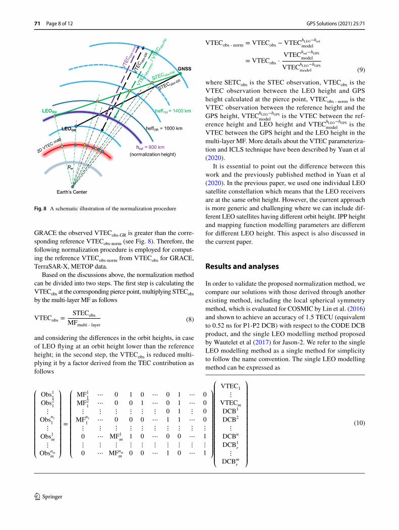
According to the discussion above, we choose 1000 km as the effective ionospheric height for GRACE and TerraSAR-X and 1400  km for COSMIC and MetOp, respectively. The intersection points between the effective height circle (labeled as heffGR and heffFM for GRACE and COSMIC, respectively) and the slant signal path, namely pierce points, determine the measurement location at which we calculate the VTECobs−norm . Since LEO satellites are flying at different orbit heights, we need a common reference height for model-ling purposes. The purple circle labeled as href = 800 km in Fig. 8 shows the reference orbit height from which the inte-gration started to compute VTECobs−norm up to GPS height for each LEO satellite mission. The schematic illustration of the normalization procedure is presented in Fig. 8. The green and black lines in solid and dashed styles in Fig. 8 represent STEC and corresponding VTEC, respectively, for COSMIC and GRACE satellites. Since COSMIC orbit height is taken as the reference height, the observed VTECobs-FM and the cor-responding reference VTECobs-norm are the same, whereas for

Fig. 7 Spatial distributions (top) and total numbers in 1 × 1 degree grids (bottom) of IPPs of topside observations for all five missions on February 2, 2013. Note that there are two symbols for two POD receivers onboard COSMIC 4. All effec-tive heights are set as 1000 km for simplicity

Table 3 Settings for parameterizing topside VTEC

Categories Settings

SHE 15-DegreeLatitude resolution 2.5°Longitude resolution 5°MF Multi-layerData source UCAR (http://cdaac -www.cosmi c.ucar.edu/

cdaac )Normalization height 800 kmEffective height 1000 km (GRACE, TerraSAR-X)

1400 km (COSMIC, MetOp)Elevation cutoff 10°Reference frame Geomagnetic reference frame (inertial)VTEC constraint 0 < VTEC < 20 (TECU)

GPS Solutions (2021) 25:71

1 3

71 Page 8 of 12

GRACE the observed VTECobs-GR is greater than the corre-sponding reference VTECobs-norm (see Fig. 8). Therefore, the following normalization procedure is employed for comput-ing the reference VTECobs-norm from VTECobs for GRACE, TerraSAR-X, METOP data.

Based on the discussions above, the normalization method can be divided into two steps. The first step is calculating the VTECobs at the corresponding pierce point, multiplying STECobs by the multi-layer MF as follows

and considering the differences in the orbit heights, in case of LEO flying at an orbit height lower than the reference height; in the second step, the VTECobs is reduced multi-plying it by a factor derived from the TEC contribution as follows

(8)VTECobs =STECobs

MFmulti - layer

where SETCobs is the STEC observation, VTECobs is the VTEC observation between the LEO height and GPS height calculated at the pierce point, VTECobs - norm is the VTEC observation between the reference height and the GPS height, VTEChLEO−hGPS

model is the VTEC between the ref-

erence height and LEO height and VTEChLEO−hGPSmodel

is the VTEC between the GPS height and the LEO height in the multi-layer MF. More details about the VTEC parameteriza-tion and ICLS technique have been described by Yuan et al (2020).

It is essential to point out the difference between this work and the previously published method in Yuan et al (2020). In the previous paper, we used one individual LEO satellite constellation which means that the LEO receivers are at the same orbit height. However, the current approach is more generic and challenging where we can include dif-ferent LEO satellites having different orbit height. IPP height and mapping function modelling parameters are different for different LEO height. This aspect is also discussed in the current paper.

Results and analyses

In order to validate the proposed normalization method, we compare our solutions with those derived through another existing method, including the local spherical symmetry method, which is evaluated for COSMIC by Lin et al. (2016) and shown to achieve an accuracy of 1.5 TECU (equivalent to 0.52 ns for P1-P2 DCB) with respect to the CODE DCB product, and the single LEO modelling method proposed by Wautelet et al (2017) for Jason-2. We refer to the single LEO modelling method as a single method for simplicity to follow the name convention. The single LEO modelling method can be expressed as

(9)

VTECobs - norm

= VTECobs

− VTEChLEO

−href

model

= VTECobs

⋅

VTEChref−h

GPS

model

VTEChLEO

−hGPS

model

(10)

⎛⎜⎜⎜⎜⎜⎜⎜⎜⎜⎝

Obs11

Obs21

⋮

Obsn11

⋮

Obs1m

⋮

Obsnmm

⎞⎟⎟⎟⎟⎟⎟⎟⎟⎟⎠

=

⎛⎜⎜⎜⎜⎜⎜⎜⎜⎜⎝

MF11

MF21

⋮

MFn11

⋮

0

⋮

0

⋯

⋯

⋮

⋯

⋮

⋯

⋮

⋯

0

0

⋮

0

⋮

MF1m

⋮

MFnmm

1

0

⋮

0

⋮

1

⋮

0

0

1

⋮

0

⋮

0

⋮

0

⋯

⋯

⋮

⋯

⋮

⋯

⋮

⋯

0

0

0

1

⋮

0

⋮

1

1

1

1

1

⋮

0

⋮

0

⋯

⋯

⋮

⋯

⋮

⋯

⋮

⋯

0

0

0

0

⋮

1

⋮

1

⎞⎟⎟⎟⎟⎟⎟⎟⎟⎟⎠

⎛⎜⎜⎜⎜⎜⎜⎜⎜⎜⎜⎜⎜⎝

VTEC1

⋮

VTECm

DCB1

DCB2

⋮

DCBn

DCB1r

⋮

DCBmr

⎞⎟⎟⎟⎟⎟⎟⎟⎟⎟⎟⎟⎟⎠

Fig. 8 A schematic illustration of the normalization procedure

GPS Solutions (2021) 25:71

1 3

Page 9 of 12 71

where Obsnmm

and MFnmm

are the phase levelled pseudorange observations and corresponding mapping functions between GPS satellite PRN nm and receiver m , VTECm is the VTEC converted at IPP of receiver m , DCBn is the satellite PRN n DCB and DCBm

r is the DCB of receiver m.

The top panel in Fig. 9 shows the daily DCB series of all 32 GPS satellites based on the single method where differ-ent colors represent different PRNs while the bottom panel shows the daily DCB series based on the normalization method. It can be seen that the GPS transmitter DCB results based on the single method are much more disturbed than those based on the normalization method. Figure 10 shows the daily difference of PRN 1–9 satellite DCBs between the normalization method and CODE as an example. The abso-lute daily difference between our results and CODE products is mostly smaller than 0.2 ns. For investigating the effect of normalization of different topside observations, we estimate the satellite and receiver DCBs with only cosmic observa-tions and all observations with a normalization procedure. Comparing the results with COSMIC only and normalization in Fig. 11, both stabilities and accuracies with normalization observations improve significantly with respect to CODE products. To evaluate the stabilities of satellite DCBs, we present the monthly standard deviations of satellite DCBs in the upper panel of Fig. 11. The median values of STDs are 0.12, 0.03, 0.39, 0.07 ns for COSMIC only, CODE, single method and normalization method, respectively. Because the DCB products are estimated based on much denser ground

networks, the stabilities of CODE products are unsurpris-ingly better than those of the normalization method. The monthly standard deviations of CODE DCB products are mostly smaller than 0.05 ns except for satellite G08, while the monthly standard deviations based on the multi-mission observations and normalization method are smaller than 0.10 ns. It is necessary to note that the standard deviation of satellite G27 (SVN G066) is missing in Fig. 9 because the RMS for G27 is 1.70 ns, which is too large to plot in the same figure. However, the monthly series of satellite DCB of G27 is quite stable as shown in Fig. 11, which means that there is an overall bias between our results and CODE

Fig. 9 Estimated GPS satellite DCBs during February 2013 based on the single method (top) and normalization method (bottom)

Fig. 10 Absolute daily difference of PRN 1–9 satellite DCBs between the normalization method and CODE

GPS Solutions (2021) 25:71

1 3

71 Page 10 of 12

products. The reason why the DCB difference for G27 is larger is that the COSMIC mission provides much fewer topside observations with G27, and the other four missions provide no topside observations with G27 at all. By checking the DCB estimate residuals provided by CODE, we found that the least-squares estimated residual of the DCB of G27 is much worse than the other GPS satellite DCBs, which may indicate a weaker performance of G27 during this period. Even though this fact could influence the DCB esti-mates through the zero-mean condition, the RMS values for other GPS satellites are still within a low value. The lower panel in Fig. 11 shows the monthly differences between GPS transmitter DCBs based on the normalization method and CODE DCB products. The root-mean-square (RMS) values of DCB differences with respect to CODE DCB products for normalization observations are mostly about 0.10 ns except for PRN 7, 19, 23, 25, 28 and 31. The median values of RMS differences are 0.19, 0.47, 0.10 ns for COSMIC only, single method and normalization method, respectively. As mentioned above, the accuracies of GPS transmitter DCB estimates based on the local spherical symmetry method for COSMIC only and based on the single method are 0.52 and 0.47 ns, respectively, while that based on the normalization method for COSMIC only is 0.19 ns. The relative improve-ments of accuracies based on the normalization method with respect to the other two methods reach 173% and 147%, respectively. Provided we combine all selected missions, the accuracies of GPS transmitter DCB estimates based on the normalization method can be further improved by 90%. It is worth noting that the most variant GPS satellite DCB (G08) in the normalization method (blue bar) coincides with that

in the CODE product (green bar), which also implies good consistency with CODE DCB product.

With the normalization method, the receiver DCBs onboard LEO satellites can be estimated simultane-ously with the GPS satellite DCBs in the normalization method. Figure 12 shows the monthly series of receiver DCBs onboard LEO satellites based on the normalization approach. The corresponding linear regression plots are superimposed on the DCB series, and the numbers represent the slope of the regression line. The differences in slopes between UCAR products and our solutions are 0.0189, 0.0078, − 0.0031, − 0.0121, 0.0047, − 0.0054 and 0.0036 ns/day, respectively. It means that the overall trends of these two DCB series are similar in the period of interest. But the DCB values estimated by UCAR are lower than those esti-mated by the normalization approach, which may be related to the inherent differences between two methods or the dif-ferent choices of mapping functions as we mention earlier in Fig. 3 that the geometric mapping function may lead to an offset away from the origin in the histogram of VTEC map-ping errors. For the TerraSAR-X satellite, DCBs estimated through the normalization approach are more variant than UCAR DCB products, which may result from two reasons. One reason is that the orbit heights of TerraSAR-X are both about 500 km. The normalization procedure for these two missions can bring more errors into DCB estimates than COSMIC and MetOp which were flying at higher altitudes of about 800 km. The other reason is that the number of observable GPS satellites for GRACE and TerraSAR-X is much lower than those of COSMIC and MetOp. Considering the two main reasons above, more fluctuating receiver DCB series onboard TerraSAR-X can be expected accordingly.

Fig. 11 Monthly STD of GPS satellite DCBs for four different cases (top panel) and RMS of GPS transmitter DCBs with respect to the CODE DCB product. (Bottom panel)

Fig. 12 Monthly series of receiver DCBs onboard LEO satellites based on the normalization approach. The corresponding linear regression plots are superimposed on the DCB series and the num-bers represent the slope of the regression line

GPS Solutions (2021) 25:71

1 3

Page 11 of 12 71

Table 4 shows the monthly standard deviation of LEO receiver DCB estimates. The standard deviations of monthly receiver DCB series of COSMIC, MetOp A/B and Ter-raSAR-X are comparable with DCB products from UCAR even without using ground-based satellite DCB products. The standard deviation differences between our solutions and UCAR products are − 0.06, 0.04, − 0.01, 0.04, 0.02, 0.07, 0.02, − 0.06 ns for COSMIC, MetOp and TerraSAR-X respectively.

Conclusion

In this study, two different kinds of mapping functions are evaluated and compared based on empirical model simula-tions. The performances of mapping functions using two different ionospheric effective height definitions are included and independently tested. The results show that the multi-layer mapping function outperforms the F&K mapping func-tion in the VTEC conversion error sense. The multi-layer MF reduced the VTEC errors resulting from horizontal electron gradient and uncertainties of effective ionospheric heights. Furthermore, a new method to estimate the GPS satellite and receiver DCBs is proposed, namely by combin-ing data from five LEO satellites at varying orbit heights and using a multi-layer mapping function (MF). We normalize the topside observations recorded at lower altitudes to those recorded at higher altitudes in order to get better coverage and observation geometry and ensure that all GPS satel-lites are observable within one day. The results show that the standard deviations of GPS transmitter DCBs based on multi-LEO observations are mostly lower than 0.10 ns (with a median value of 0.07 ns) and the GPS satellite DCB solu-tions based on multi-LEO observations are close to those of the CODE DCB product with an RMS value of 0.10 ns. The relative improvements of accuracies based on the normaliza-tion method with respect to the other two existing methods, namely the single method and local spherical symmetry

method, are 173% and 147%, respectively. Provided we combine topside observations from all selected missions, the accuracies of GPS transmitter DCB estimates based on the normalization method can be further improved by 90% with respect to those using only COSMIC observations .

The receiver DCBs onboard LEO satellites are estimated simultaneously with the GPS satellite DCBs with the nor-malization method. The stabilities of estimated receiver DCBs onboard COSMIC and MetOp missions are com-parable with those provided by UCAR even without using ground-based satellite DCB products, which indicates the potential of the normalization method to derive better receiver DCB products with more topside observations in the future.

Acknowledgements We thank the UCAR/CDAAC data centre for pro-viding the precise orbit determination data of COSMIC, METOPA, METOPB, GRACE and TerraSAR-X. This study was supported by the National Natural Science Foundation of China (NSFC) Project Grant Numbers 41761134092.

Funding Open Access funding enabled and organized by Projekt DEAL.

Data availability Data from all LEO missions used in this study can be found at the UCAR/CDAAC data centre http://cdaac -www.cosmi c.ucar.edu/cdaac . The model simulation data in this manuscript can be provided by the corresponding author on request.

Open Access This article is licensed under a Creative Commons Attri-bution 4.0 International License, which permits use, sharing, adapta-tion, distribution and reproduction in any medium or format, as long as you give appropriate credit to the original author(s) and the source, provide a link to the Creative Commons licence, and indicate if changes were made. The images or other third party material in this article are included in the article’s Creative Commons licence, unless indicated otherwise in a credit line to the material. If material is not included in the article’s Creative Commons licence and your intended use is not permitted by statutory regulation or exceeds the permitted use, you will need to obtain permission directly from the copyright holder. To view a copy of this licence, visit http://creat iveco mmons .org/licen ses/by/4.0/.

References

Anthes RA et  al (2008) The COSMIC/FORMOSAT-3 mission: early results. Bull Am Meteorol Soc 89:313–333. https ://doi.org/10.1175/BAMS-89-3-313

Bilitza D (2001) International reference ionosphere 2000. Radio Sci 36:261–275. https ://doi.org/10.1029/2000R S0024 32

Brunini C (2011) Simulation study of the influence of the ionospheric layer height in the thin layer ionospheric model. J Geodesy 85:637–645

Bartalis Z, Wagner W, Naeimi V, Hasenauer S, Scipal K, Bonekamp H, Figa J, Anderson C (2007) Initial soil moisture retrievals from the METOP-A advanced Scatterometer (ASCAT). Geophys Res Lett 34(20):L20401

Foelsche U, Kirchengast G (2002) A simple ‘“geometric”’ map-ping function for the hydrostatic delay at radio frequencies and

Table 4 Comparisons of LEO receiver DCBs stabilities between the normalization method and UCAR DCB products. Note that due to the discontinuity of GRACE POD data, the monthly standard deviation of receiver DCB onboard GRACE is not shown here

Receiver UCAR STD (ns) Norm STD (ns)

C1POD1 0.14 0.20C2POD1 0.23 0.19C4POD0 0.17 0.18C5POD1 0.14 0.10C6POD1 0.14 0.12METOPA 0.14 0.07METOPB 0.09 0.07TerraSAR-X 0.07 0.13

GPS Solutions (2021) 25:71

1 3

71 Page 12 of 12

assessment of its performance. Geophys Res Lett 29:1473. https ://doi.org/10.1029/2001G L0137 44

Gallagher DL, Craven PD, Comfort RH (2000) Global core plasma model. J Geophys Res 105:18819–18833. https ://doi.org/10.1029/1999J A0002 41

Hernández-Pajares M, Juan JM, Sanz J, Orus R, Garcia-Rigo A, Feltens J, Komjathy A, Schaer SC, Krankowski A (2009) The IGS VTEC maps: a reliable source of ionospheric information since 1998. J Geod 83:263–275. https ://doi.org/10.1007/S0019 0-008-0266-1

Hoque MM, Jakowski N (2007) Mitigation of higher order ionospheric effects on GNSS users in Europe. GPS Solut 12(2):87–97. https ://doi.org/10.1007/s1029 1-007-0069-5

Hoque MM, Jakowski N (2011) A new global empirical NmF2 model for operational use in radio systems. Radio Sci 46(6):1–13

Hoque MM, Jakowski N (2012) A new global model for the iono-spheric F2 peak height for radio wave propagation. Ann Geophys 30(5):797–809

Hoque MM, Jakowski N (2013) Mitigation of ionospheric mapping function error. In: Proceedings of ION GNSS + 2013, Institute of Navigation, Nashville, Tennessee, USA, September 16–20, 1848–1855

Huang Z, Yuan H (2013) Analysis and improvement of ionospheric thin shell model used in SBAS for China region. Adv Space Res 51:2035–2042

Jakowski N, Wehrenpfennig A, Heise S, Reigber C, Lühr H, Grunwaldt L, Meehan TK (2002) GPS radio occultation measurements of the ionosphere from CHAMP: early results. Geophys Res Lett 29(10):1457. https ://doi.org/10.1029/2001G L0143 64

Jakowski N, Hoque MM, Mayer C (2011) A new global TEC model for estimating transionospheric radio wave propagation errors. J Geod 85(12):965–974

Lanyi GE, Roth T (1988) A comparison of mapped and measured total ionospheric electron content using global positioning system and beacon satellite observations. Radio Sci 23:483–492

Li W, Li M, Shi C, Fang R, Bai W (2017) GPS and BeiDou differential code bias estimation using Fengyun-3C satellite onboard GNSS observations. Remote Sens 9:1239

Lin J, Yue X, Zhao S (2016) Estimation and analysis of GPS satellite DCB based on LEO observations. GPS Solut 20:251–258

Mannucci A, Wilson B, Yuan D, Ho C, Lindqwister U, Runge T (1998) A global mapping technique for GPS-derived ionospheric total electron content measurements. Radio Sci 33(3):565–582

Rishbeth H, Garriott OK (1969) Introduction to ionospheric physics. Academic Press, New York

Schaer S, Beutler G, Rothacher M (1998) Mapping and Predicting the Ionosphere. In: Dow JM, Kouba J, Springer T (eds) Proceed-ings of the 1998 IGS analysis center workshop, Darmstadt. ESA/ESOC, Darmstadt, pp 307–318

Spilker JJ (1991) Tropospheric effects on GPS Global Positioning Sys-tem. Theory Appl 1:517–546

Tapley BD, Bettadpur S, Watkins M, Reigber C (2004) The grav-ity recovery and climate experiment: mission overview and early results. Geophys Res Lett 31:L09607. https ://doi.org/10.1029/2004G L0199 20

Wautelet G, Loyer S, Mercier F, Perosanz F (2017) Computation of GPS P1–P2 differential code biases with JASON-2. GPS Solut 21:1–13

Xiang Y, Gao Y (2019) An enhanced mapping function with iono-spheric varying height. Remote Sens 11:1497

Yuan L, Jin S, Hoque M (2020) Estimation of LEO-GPS receiver dif-ferential code bias based on inequality constrained least square and multi-layer mapping function. GPS Solut 24:57

Zhong J, Lei J, Dou X, Yue X (2016a) Assessment of vertical TEC mapping functions for space-based GNSS observations. GPS Solut 20(3):353–362

Zhong J, Lei J, Yue X, Dou X (2016b) Determination of differential code bias of GNSS receiver onboard low earth orbit satellite. IEEE Trans Geosci Remote Sens 54:4896–4905

Publisher’s Note Springer Nature remains neutral with regard to jurisdictional claims in published maps and institutional affiliations.

Liangliang Yuan received his Bachelor in Space Science and Technology in 2016 from Nan-jing University, Nanjing, China, and his Ph.D. degree in Astrom-etry and Celestial Mechanics in 2020 from the Shanghai Astro-nomical Observatory, Chinese Academy of Sciences, Shanghai, China. He has been working at the Space Weather Observations department at the DLR Institute for Solar-Terrestrial Physics since 2020. His research inter-ests include GNSS ionospheric radio occultation and thermo-

sphere-ionosphere coupling.

M o h a m m e d M a i n u l Hoque received his Bachelor in Electrical and Electronics Engi-neering in 2000 and was awarded a Ph.D. in 2009 from the Univer-sity of Siegen, Germany. He has been working on ionospheric modelling, including higher order propagation effects at the German Aerospace Center (DLR) since 2004. Since 2019 he is the head of the Space Weather Observations depart-ment at the DLR Institute for Solar-Terrestrial Physics.

Shuanggen Jin is a Professor and Group Head at the Shanghai Astronomical Observatory, CAS. His main research areas include  Satellite Navigation, Space Geodesy, Remote Sens-ing, Climate Change and Space/Planetary Exploration. He has received 100-Talent Program of CAS, Fellow of IAG, Fellow of IUGG, Member of Russian Academy of Natural Sciences and Member of European Acad-emy of Sciences.