A New GIS based Mountain Permafrost Distribution Model Lukas U. Arenson & Matthias Jakob BGC Engineering Inc., Vancouver, BC, Canada ABSTRACT A new GIS supported mountain permafrost distribution model has been developed that is based on statistical analysis of morphologic terrain expressions from field observations and interpretations of aerial photographs and satellite images. Elevation, slope aspect, potential solar radiation and slope angles are determined from a digital elevation model within GIS and relationships for the possible or likely occurrence of permafrost developed. These relationships are used to create a permafrost distribution map that designates areas of possible and likely permafrost. The modular structure of the model allows continuous model improvements as new field observations become available as a project progresses. RÉSUMÉ Un nouveau modèle de distribution de pergélisol de montagne a été développé dans SIG sur la base d'analyse statistique des expressions de terrain morphologique d'observations, photos aérienne et images satellite. L’élévation, les aspects de pente, la pénétration du soleil et les inclinations de pente sont déterminées à partir d'un modèle numérique d'élévation dans SIG et les relations sont développées pour l'apparition possible ou susceptible de pergélisol. Ces relations sont utilisées pour créer une carte de distribution de pergélisol. La structure modulaire du modèle permet des améliorations continues comme nouvel essais in situ et observations sont disponibles au fur d’un projet avance. 1 INTRODUCTION It is desirable and sometimes essential in high altitude projects to understand the spatial distribution of mountain permafrost. Environmental and geohazard risk assessments as well as geotechnical design require information on the distribution, morphologic expressions and thermodynamics of permafrost. During recent years construction activities, in particular mining and related infrastructure, have advanced into increasingly high altitudes where frozen ground is encountered. The remoteness of those areas is responsible for the paucity of information on permafrost. For this reason a standardized and replicable scientifically-defensible method to predict permafrost distribution that relies on remotely sensed data and field observations is in high demand.

In mountainous terrain, permafrost distribution and ground temperature regime vary with Quaternary and especially Holocene landscape evolution, elevation, solar radiation, surface material properties and local micro-meteorological characteristics such as cold-air drainage and local inversions. A regional permafrost prediction model that requires integration of these variables would not be practical since often ground surface and subsurface temperatures can only be measured at a later stage of infrastructure development.

Permafrost distribution models have been developed during the last decade by research institutions (e.g. Etzelmüller et al. 2001, Gruber et al. 2003, 2004, Hoelzle et al. 2005, Etzelmüller et al. 2006, Riseborough et al. 2008). In contrast to high latitude permafrost distribution models outside of mountain ranges, topography is fundamental to the formation and preservation of permafrost. Universities in Europe (e.g. Zurich, Oslo) have been leading this research. However, the use of such models for practical applications can be expanded.

User interaction and incorporating professional judgment at various stages during the modeling process are restricted in these models. For example, it is difficult to utilize information that may become available as a project advances. Initially, only remote data might be available, followed by some field inspections for surface terrain types and later complemented by monitoring data, such as soil stratigraphy, ground temperature data and detailed climate records. User interfaces and often simple means of incorporating new data as they become available are required. In addition, the user should have the option of manually calibrating the model to make changes based on local knowledge. If areas that have been selected by the model as potentially underlain by permafrost are known to have no permafrost, they should be excluded manually and this knowledge should be incorporated in the model to find similar locations. Such a model would be desirable for industry application. Furthermore it would be beneficial if a permafrost distribution model would facilitate the integration of geomorphic permafrost indicators, ground temperature data or test pit observations.

To account for some of these shortcomings a new GIS-supported permafrost distribution model is under development that is based on statistical analysis of morphologic permafrost indicators, air photo and satellite image interpretation, and climatic and morphometric parameters calculated from digital elevation models (DEM).

This paper summarizes the model design and its results based on an arbitrarily chosen area in the Andes. Because of proprietary data it is not yet possible to present examples where initial model results were confirmed with field observations.

452

2 BASIC MODEL STRUCTURE The topography affects permafrost presence and distribution through its influence on the solar radiation that also controls the subsurface energy flux. Noetzli and Gruber (2009) demonstrate that past climates are still affecting present-day permafrost temperatures. Local conditions are thus to be integrated in permafrost distribution models.

The model presented herein is primarily based on physical evidence, in particular remote sensing data and field observations. Areas potentially underlain by permafrost, such as rock glaciers, gelifluction slopes, test pits, pattern ground or creeping slopes, are statistically analysed. Such approach has been successfully applied in several regions, in particular where only sparse data were available for remote areas (Riseborough et al. 2008).

Elevation, slope aspects, potential solar radiation and slope angles are determined in a GIS environment for areas underlain by permafrost. Solar radiation and aspect are the principal factors influencing formation of permafrost in mountainous environments (Gruber 2005) and should be weighted more than the other parameters. In addition, broad regional variations are considered by analysing longitudinal and latitudinal trends. With a DEM it is then possible to formulate general relationships for permafrost occurrence. These are subsequently used within GIS to model the mountain permafrost distribution and create a map.

Three classes of permafrost are distinguished in this model, according to known classifications (e.g. Haeberli 1973): • Likely Permafrost

Most of this area is expected to be underlain by permafrost.

• Possible Permafrost Depending on the local surface characteristics and topography permafrost is expected. Large bodies of permafrost as well as areas with only isolated patches are possible. However, no thick (> 20m) and continuous permafrost layers are expected.

• No Permafrost Generally, no permafrost is expected in these areas. However, sporadic exceptions are possible due to local microclimatic conditions. Rock glaciers, for example, have been reported at mean annual air temperatures (MAAT) of +4°C (Kammer 1998).

Satellite Images

Air Photos

DEM

Test Pits

Terrain Type

Remote Sensing Data

Field Observations

Site Investigation

Monitoring

Boreholes Geophysics

Surface Geomorphology- Rock Glaciers- Gelifluction Slope- Pattern Ground- …

Stratigraphy

Soil Conditions

Ground Ice Content

Climate DataGround

Temperature

Surface Deformation

Internal Deformation

N-Factors

Ground Thermal Properties

Ground Movements / activity

Elevation

Slope Angles

Solar Radiation

Aspect

Relationships

Model- No Permafrost- Permafrost Possible- Permafrost Likely

Ground Truthing

LiDAR

Geomorphology

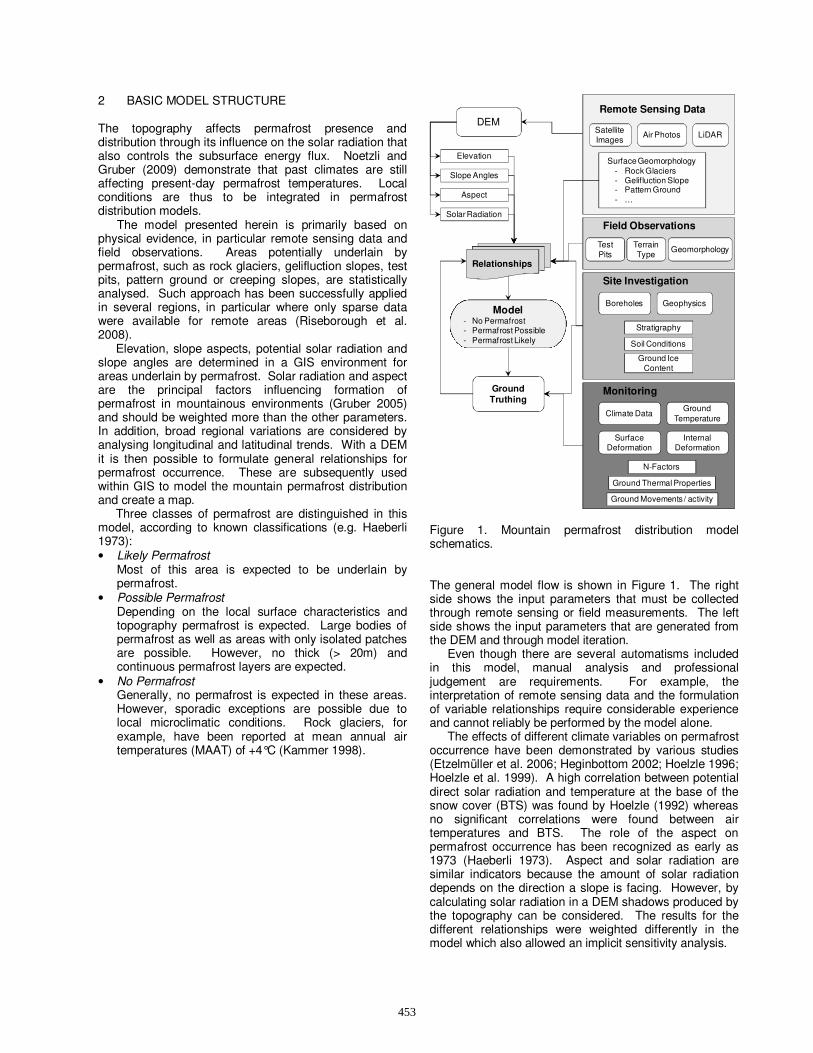
Figure 1. Mountain permafrost distribution model schematics. The general model flow is shown in Figure 1. The right side shows the input parameters that must be collected through remote sensing or field measurements. The left side shows the input parameters that are generated from the DEM and through model iteration.

Even though there are several automatisms included in this model, manual analysis and professional judgement are requirements. For example, the interpretation of remote sensing data and the formulation of variable relationships require considerable experience and cannot reliably be performed by the model alone.

The effects of different climate variables on permafrost occurrence have been demonstrated by various studies (Etzelmüller et al. 2006; Heginbottom 2002; Hoelzle 1996; Hoelzle et al. 1999). A high correlation between potential direct solar radiation and temperature at the base of the snow cover (BTS) was found by Hoelzle (1992) whereas no significant correlations were found between air temperatures and BTS. The role of the aspect on permafrost occurrence has been recognized as early as 1973 (Haeberli 1973). Aspect and solar radiation are similar indicators because the amount of solar radiation depends on the direction a slope is facing. However, by calculating solar radiation in a DEM shadows produced by the topography can be considered. The results for the different relationships were weighted differently in the model which also allowed an implicit sensitivity analysis.

453

3 EXAMPLE OF PERMAFROST DISTRIBUTION MODEL

An example in which only remotely sensed data was entered is presented to illustrate the permafrost distribution model. The study area is about 1,140 km2 and located at the Argentine – Chilean boarder, 31.6 °S (Figure 1).

Figure 2. Location of the study area used for the model example. 3.1 GIS Calculated Data A DEM was generated with a 30 m resolution ASTER GDEM data set that became publically available in June, 2009. Elevation, slope angle, slope aspect and total, yearly incoming solar radiation were determined for each raster point in the study area. The solar radiation tool in the ArcGIS Spatial Analyst extension accounts for atmospheric effects, site latitude and elevation, steepness and aspect, daily and seasonal shifts of the sun angle, and effects of shadows cast by surrounding topography (ESRI 2009). Clear sky conditions were applied in these calculations which, for the selected site, is a reasonable approximation. In total more than 1.3 Million data points are used for the study area. 3.2 Surface Geomorphology Permafrost indicators were identified using Landsat 5 and Landsat 7 images, which are freely available through the U.S. Geological Survey (USGS) and the National Aeronautics and Space Administration (NASA). These images have a spatial resolution of 30 m for the reflective bands and Landsat 7 produces a 15 m panchromatic band allowing a better identification of surface features.

The geomorphic surface indicators for permafrost conditions that can be identified from these satellite images are rock glaciers and gelifluction slopes and in some cases pattern grounds. It is often not possible to

determine whether a rock glacier is active or not. Chronosequential images can help to identify rock glacier activity by examining movement of individual boulders on the rock glacier surface. Both the lower elevation of characteristic ribbons of gelifluction slopes and the lower limit of rock glaciers are used to create relationships for mountain permafrost occurrence. 3.3 Relationships The remotely sensed data are compared with the parameters from the GIS model to determine relationships that feed the permafrost distribution model. Five different relationships are developed within this model. Permafrost occurrence as a function of:

1. Slope aspect; 2. Solar Radiation; 3. Slope Angle; 4. Easting; and 5. Northing.

Nearly 4,000 raster points (about 30 m x 30 m) were analysed based on the geoforms identified. Approximately 25% were gelifluction slopes, and 75% rock glaciers, which were easier to identify on the satellite images. Figures 3a to 3e show these data points in various variable dependencies. The solid lines indicate the envelopes applied to distinguish the possible and likely occurrence of permafrost. The difference in elevation between the possible permafrost and likely permafrost occurrence was chosen to be constant (50 m) for this model. The value is based on the data distribution shown in Figure 3.

The slope aspect affects the likelihood for permafrost occurrence through radiative forcing with north-facing slopes (0/360° aspect) showing permafrost existence at 300 m higher elevations than south-facing slopes (180° aspect). The reason behind this difference is the significant difference in solar radiation between these slope aspects. A cluster of data point in Figure 3a is located below the possible permafrost boundary at slope aspects between 0° and 60°. These data originate from a gelifluction slope. It was decided to not include these points due to the uncertainties whether this slope is currently still underlain by permafrost or not. Relict gelifluction slopes may still be visible in the area due to low surface erosion rates. In particular the lack in similar data for slope aspects ranging between 300° and 360° supported this judgment.

Areas with total yearly incoming solar radiations of greater or equal 2.5 MW/m2 did not indicate permafrost and can be delineated accurately.

In the original rule of thumb on Alpine permafrost presented by Haeberli (1973), slopes flatter and steeper than 11° were given different criterions. Within our model, the slope was incorporated as an independent variable. Our analyses confirmed that below about 10°, permafrost elevation changes as a function of the slope gradient are insignificant.

454

3300

3400

3500

3600

3700

3800

3900

4000

4100

4200

4300

0 60 120 180 240 300 360

Ele

vati

on

(m

AS

L)

Aspect (°)

3300

3400

3500

3600

3700

3800

3900

4000

4100

4200

4300

1.0E+06 1.5E+06 2.0E+06 2.5E+06 3.0E+06

Ele

va

tio

n (

m A

SL)

Total Solar Radiation (W/m2 yr)

(a) Slope aspect versus elevation. (b) Solar radiation versus elevation.

3300

3400

3500

3600

3700

3800

3900

4000

4100

4200

4300

0 10 20 30 40

Ele

vat

ion

(m

AS

L)

Slope Angle (°) (c) Slope angle versus elevation.

3300

3400

3500

3600

3700

3800

3900

4000

4100

4200

4300

330,000 340,000 350,000 360,000 370,000 380,000 390,000

Ele

vati

on

(m

ASL

)

Easting (UTM)

3300

3400

3500

3600

3700

3800

3900

4000

4100

4200

4300

6,490,000 6,495,000 6,500,000 6,505,000 6,510,000

Ele

va

tio

n (

m A

SL

)

Northing (UTM)

(d) Easting versus elevation (UTM 19J, WGS 84). (e) Northing versus elevation (UTM 19J, WGS 84).

Figure 3. Model relationships based on surface geomorphic indicators identified from satellite images. A total of about 4,000 points are analysed. The black line is the lower boundary of likely permafrost and the grey line the lower boundary for possible permafrost. The difference was selected to be 50 m and independent of the various parameters for this initial analysis.

455

Finally, a regional climatic variable is included to account for latitudinal or continental effects. These variables are entered simply by the geographic location, of a particular point. The envelope is chosen by considering the trends in the minimum elevation. The plots show the change in aspect along the east-west and north-south transects. In particular the difference between permafrost occurrence of north-facing slopes and south-facing slopes can clearly be noted in Figure 3d. No significant trend is seen in a north-south direction (Figure 3e), but a notable effect exists from east to west (Figure 3d). We explain the latter by increasing continentality towards Argentina. Variability is likely introduced by meso-scale climatic characteristics.

Table 1 provides an overview of how many of the identified raster points fall within the three classes using the relationships developed for this model. The parameters in the relationships for the envelopes shown in Figures 3a to Figure 3e were chosen so that about 90% of the identified permafrost indicators fall within the permafrost likely zone. This is an initial selection and considered to be a conservative assumption for Environmental Impact Assessments (EIA) and preliminary design work. 5% of the “aspect” points (Figure 3a) and 9% of the “solar radiation” points (Figure 3b) that were identified as permafrost indicators from satellite images are located outside the selected permafrost envelopes. In total, only about 1% of the identified permafrost landform raster points are located in the non-permafrost zone. Table 1. Overview of model input data accuracy: Percentage of raster points identified from satellite images as being located in a permafrost zone that fall within the permafrost envelopes shown in Figure 3. Characteristics Rock Glaciers Gelifluction

No permafrost (%) 1 2

Permafrost possible (%) 8 9

Permafrost likely (%) 91 89

3.4 Model Results Based on the relationships shown in Figure 3, five layers are created, in which each raster point is identified as being located in non-permafrost, possible permafrost or likely permafrost. A value of either 0, 1, or 2 is then assigned for each of the above categories. The different layers are weighted and added to create the final distribution map. Each layer was given a weight value, W…, between 0 and 1 with which the permafrost likelihood, V…, value is multiplied: V = Wa·Va + Wsr·Vsr + Ws·Vs + Wn·Vn + We·Ve [1] The sum of the weights equals 1.0. Only raster points with a total value V of 2 (i.e. meeting all criteria), were designated as likely permafrost locations. Values of V between 1 and 2 were classified as possible permafrost and all other values are classified as non-permafrost occurrence. This process is schematically shown in Figure 4. The weights for aspect, Wa, solar radiation, Wsr,

slope angle, Ws, northing, Wn, and easting, We, are assigned based on professional judgement and experience. A sensitivity analysis was carried out to test the sensitivity of these weights.

The distribution of the final permafrost likely values V is presented in Figure 5 as a map for a larger area and in Figure 6 as one particular mountain ridge. A well developed lobate rock glacier in the center of the second figure can be identified that is assigned as permafrost likely terrain. The model outlines the extension of this rock glacier reasonably well. The adjacent areas are assigned as possible permafrost.

Sat Image

Aspect

Solar

Radiation

Slope

East

North

Figure 4. Schematic representation of layer addition. Each layer is multiplied by a weight W… to obtain the final layer shown in Figure 5.

0 3 61.5 Kilometers

Figure 5. Mountain permafrost distribution map. The dark blue areas indicate permafrost likely and the light blue permafrost possible, respectively. The relationships are based on satellite image analysis only.

456

Figure 6. 3D view of a mountain ridge with the mountain permafrost distribution map overlay. The dark blue areas indicate permafrost likely and the light blue permafrost possible, respectively. The relationships are based on satellite image analysis only. Note the lobate rock glacier in the centre of the figure. 3.5 Model Sensitivity In order to assess the model sensitivity, six different weight combinations were tested. By changing the weightings some input parameters become more important than others. The different combinations are summarized in Table 2. Table 2. Weighting factor combinations used in sensitivity analysis. Case Aspect SR Slope Easting Northing

1 1/5 1/5 1/5 1/5 1/5

2 1/3 1/6 1/6 1/6 1/6

3 1/4 1/4 1/6 1/6 1/6

4 1/6 1/3 1/6 1/6 1/6

5 1/6 1/6 1/3 1/6 1/6

6 1/4 1/4 1/4 1/8 1/8

The modeling results from the sensitivity analysis were evaluated by comparing the fraction of all points identified as permafrost / non-permafrost between the different weighting factor combinations. There are only minor differences in the total distribution (Table 3). Because all criteria have to be met in order for a raster point to be identified as permafrost likely, this value stays at 32.1%. The sum of the weighting factors is 1.0 and all permafrost values V… are 2.0, hence changes in W… do not affect the result.

But even changes in the weighting factors only have a minor influence on the model output. The smallest permafrost area is predicted if the aspect is weighted the highest (Case 2: Wa = 0.33). As shown by Gruber (2005), aspect and solar radiation are the two most important parameters. Therefore, Case 3, where the two make 50% of the total weighting, was selected as the most likely

permafrost distribution. Weightings can also be easily updated within this model as more data become available in the future. Table 3. Percentages of permafrost likely, permafrost possible and no permafrost for different weightings. Case No

Permafrost Permafrost Possible

Permafrost Likely

Permafrost Pos. + Lik.

1 50.6 % 17.3 % 32.1 % 49.4%

2 51.6 % 16.3 % 32.1 % 48.4%

3 51.4 % 16.5 % 32.1 % 48.6%

4 51.1 % 16.8 % 32.1 % 48.9%

5 51.3 % 16.6 % 32.1 % 48.7%

6 51.3 % 16.6 % 32.1 % 48.7%

4 DISCUSSION With most models, the quality and quantity of the input data are most critical and control the complexity of a model. The fewer data available, the less complex a model should be, primarily because the cases needed to provide statistically significant results are not available. For the permafrost distribution model presented, where only limited data from remote sensing sources are available for input, model complexity should be moderate. No ground temperatures are available that allow determination of geothermal gradients, permafrost thicknesses or spatial changes in the ratio between air temperature and ground surface temperature, i.e. information on the local surface energy balance (SEB). Furthermore, no detailed information on the snow cover distribution are available that could be used in a more complex SEB model. There is also only limited information available on the material properties of the ground that could be used in estimating latent heat effects and thermal conductivities. Changes in the ground surface characteristics can cause differences in the mean annual ground temperature of 5 to 10°C (Andersland and Ladanyi 2004) and strongly affect the local potential for permafrost formation and protection.

The new model presented only predicts classes for permafrost likelihood and not a continuous probability scale to reflect these variabilities and uncertainties. In reality these boundaries are not sharp, but gradual. Complex three-dimensional thermo-topographic effects, such as thermal anomalies or wind-related snow accumulation on leeward slopes around steep mountain ridges, in narrow valleys or snow avalanche fans, and transient climate conditions are not considered.

Even though this initial modeling approach is primarily based on surface indicators, the chosen relationships provide a reasonably reliable permafrost distribution model of the study area. As more data become available, particularly for areas where regulators demand a higher data density from mine developers, such as ground temperatures, ice contents, soil characteristics and thermal properties, the model complexity can be increased. The model errors can be better quantified and

457

progressively reduced. The modular structure and model interaction possibilities allow for a continuous model update and manual refinement. We caution against ignorance of professional judgment and warn against overrating the role of model automatisms. 5 CONCLUSIONS A new mountain permafrost distribution model is presented that functions as a multi-layer data analysis tool. Initially only indirect, geomorphic surface indicators are used within a GIS framework. Areas are first identified from remote sensing data as being potentially underlain by permafrost, such as rock glaciers and slopes characterized by gelifluction lobes. Elevation, slope aspect, potential solar radiation, slope angle, and regional effects are determined within GIS and compared with the interpreted areas of permafrost. Solar radiation and aspect are the two most important factors that affect permafrost existence in mountainous environments and therefore a weighting of the input factors was included. Hence, 50% of the total weight was given these two elements. The results of this model are only a first estimate. No ground temperature data were available as input parameters for the model and no effects of the terrain type have been considered. Yet, this distribution model provides a valuable approximation of permafrost occurrence that can be used for initial project planning and specific permafrost site investigations. It is efficient and can be applied for large study areas, but still relies upon and incorporates professional judgement.

The major advantage of the model is its capability for regular refinements as new field observations become available during site investigations, which increase the confidence in the model output as a project progresses. ACKNOWLEDGEMENTS The authors would like to thank Jamie Sorensen for the GIS modeling and Michael Porter for reviewing the manuscript. The support by BGC Engineering Inc. in providing the opportunity to develop this model is further acknowledged. REFERENCES Andersland, O.B., Ladanyi, B. 2003. An Introduction to

Frozen Ground Engineering. 2nd ed. ASCE & John Wiley & Sons, New York, NY, USA.

ESRI 2009. ArcGIS Desktop 9.3.1. Spatial Analyst Tools. http://www.esri.com.

Etzelmüller, B., Hoelzle, M., Heggem, E.S.F., Isaksen, K., Mittaz, C., Vonder Mühll, D., Ødegård, R.S., Haeberli, W., Sollid, J.L. 2001. Mapping and modelling the occurrence and distribution of mountain permafrost. Norwegian Journal of Geography, 55: 186–194.

Etzelmüller, B., Heggem, E.S.F., Sharkhuu, N., Frauenfelder, R., Kääb, A., Goulden, C.E. 2006. Mountain permafrost distribution modelling using a multi-criteria approach in the Hövsgöl area, Northern Mongolia. Permafrost and Periglacial Processes, 17: 91–104.

Gruber, S., Peter, M., Hoelzle, M., Woodhatch, I., Haeberli,W. 2003. Surface temperatures in steep alpine rock faces - a strategy for regional-scale measurement and modelling. In: Phillips, M., Springman, S.M., Arenson, L.U. (Eds.), Proceedings 8th International Conference on Permafrost. Swets and Zeitlinger, Lisse: 325–330.

Gruber, S., Hoelzle, M., Haeberli, W. 2004. Rock-wall temperatures in the Alps: modelling their topographic distribution and regional differences. Permafrost and Periglacial Processes, 15: 299–307.

Gruber, S. 2005. Mountain permafrost: Transient spatial modelling, model verification and the use of remote sensing. PhD Thesis, Universität Zürich, Zürich.

Haeberli, W. 1973. Die Basis-Temperatur der winterlichen Schneedecke als möglicher Indikator für die Verbreitung von Permafrost in den Alpen. Zeitschrift für Gletscherkunde und Glazialgeologie. Universitätsverlag Wagner – Innsbruck: 221–227.

Heginbottom, J. A. 2002. Permafrost mapping: a review. Progress in Physical Geography, 26(4): 623-642.

Hoelzle, M. 1992. Permafrost occurrence from BTS measurements and climatic parameters in the eastern Swiss Alps. Permafrost and Periglacial Processes, 3(2): 143-147.

Hoelzle, M. 1996. Mapping and modelling of mountain permafrost distribution in the Alps. Norwegian Journal of Geography, 50: 11–15.

Hoelzle, M., Wegmann, M., Krummenacher, B. 1999. Miniature temperature data loggers for mapping and monitoring of permafrost in high mountain areas: first experience from the Swiss Alps. Permafrost and Periglacial Processes, 10: 113–124.

Hoelzle, M., Mittaz, C., Etzelmüller, B., Haeberli, W. 2001. Surface energy fluxes and distribution models of permafrost in European mountain areas: an overview of current developments. Permafrost and Periglacial Processes, 12 (1): 53–68.

Hoelzle, M., Paul, F., Gruber, S., Frauenfelder, R. 2005. Glacier and permafrost in mountain areas: different modelling approaches. Projecting Global Change Impact and Sustainable Land use and Natural Resource Management in Mountain Biosphere Reserves (GLOCHAMORE). Global Change Impacts in Mountain Biosphere Reserves. UNESCO, Paris: 28–39.

Kammer, K. 1998. Rock glacier inventory western Andes, Chile. http://nsidc.org/data/docs/fgdc/ggd282_ rockglac_chile/index.html.

Riseborough, D., Shiklamonov, N.I., Etzelmüller, B., Gruber, S., Marchengo, S. 2008. Recent advances in permafrost modeling. Permafrost and Periglacial Processes, 19 (2): 137–156.

USGS 1999: Glaciers of the dry Andes. http://pubs.usgs.gov/prof/p1386i/chile-arg/dry/ index.html

458