Embed Size (px)
Citation preview

A New Decision Theoretic Sampling Plan for
Exponential Distribution under Type-I Censoring
Deepak Prajapati∗& Sharmistha Mitra†& Debasis Kundu‡
Abstract
In this paper a new decision theoretic sampling plan (DSP) is proposed for Type-I
censored exponential distribution. The proposed DSP is based on a new estimator of
the expected lifetime of an exponential distribution which always exists, unlike the
usual maximum likelihood estimator. The DSP is a modification of the Bayesian vari-
able sampling plan of Lam (1994). An optimum DSP is derived in the sense that it
minimizes the Bayes risk. In terms of the Bayes risks, it performs better than Lam’s
sampling plan and its performance is as good as the Bayesian sampling plan of Lin,
Liang and Haung (2002), although implementation of the DSP is very simple. Ana-
lytically it is more tractable than the Bayesian sampling plan of Lin, Liang and Haung
(2002), and it can be easily generalized for any other loss functions also. A finite algo-
rithm is provided to obtain the optimal plan and the corresponding minimum Bayes
risk is calculated. Extensive numerical comparisons with the optimal Bayesian sam-
pling plan proposed by Lin, Liang and Haung (2002) are made. The results have been
extended for three degree polynomial loss function and for Type-I hybrid censoring
scheme.
∗Department of Mathematics and Statistics, Indian Institute of Technology Kanpur, India†Department of Mathematics and Statistics, Indian Institute of Technology Kanpur, India‡Department of Mathematics and Statistics, Indian Institute of Technology Kanpur, India, Corresponding
author, e-mail: [email protected].
1

2
Keywords and Phrases: Bayesian sampling plan, Exponential distribution, Type-I censor-
ing, Proposed estimator, Bayes risk.
1 Introduction
In statistical quality control, acceptance sampling plans play a crucial role in deciding
whether to accept or reject a batch of products. There are various approaches to deter-
mine these sampling plans. Both classical and decision theoretic approaches have been
discussed in the literature. From the point of view of economy, the decision theoretic
approach is more scientific and realistic because the sampling plan is determined by mak-
ing an optimal decision on the basis of some economic consideration such as maximizing
the return or minimizing the loss. Extensive work has been done dealing with the de-
signing of the sampling plans under different censoring schemes. See for example Hald
(1967), Fertig and Mann (1974), Thyregod (1975), Wetherill and Kollerstrom (1979), Lam
(1988, 1990), Lam and Choy (1995), Huang and Lin (2002), Lin, Huang and Balakrishnan
(2008a,b), Liang and Yang (2013), Tsai et al. (2014), Chen, Yang and Liang (2015) and the
references cited therein.
In practice, life testing experiments are usually censored in the sense that the test-
ing procedure terminates before the actual lifetime of all selected items are observed. Lam
(1994) investigated this problem of formulating sampling plans for the exponential distri-
bution with Type-I censoring. The one-sided decision function is based on the maximum
likelihood estimator (MLE) of the expected lifetime, when it exists. The sampling plan is
a triplet (n,τ,ξ ) where n is the number of items inspected, τ is the fixed censoring time
and ξ is the minimum acceptable surviving time, i.e., the lot is accepted if and only if the
maximum likelihood estimate of the expected lifetime is larger than or equal to ξ .
In this approach, there are two shortcomings which should be mentioned. First
of all, under a Type-I censoring, the MLE of the expected lifetime may not always exist.

3
Secondly, the loss function of Lam (1994) consists of the sampling cost and a component
of the polynomial decision loss function only. Lin, Liang and Haung (2002) first observed
that Lam (1994) does not take the cost of the testing time τ into account in the loss func-
tion. In fact, they rightly observed that taking τ = ∞, the sampling plan proposed by them
gives better results than the sampling plan of Lam (1994). It indicates that if we do not
consider the cost of the testing time in the loss function then it leads to wrong results.
By considering a Bayes decision function which minimizes Bayes risk over optimal (n,τ),
Lin, Liang and Haung (2002) showed that the sampling plan of Lam (1994) is “neither
optimal, nor Bayes”. From now on the sampling plan proposed by Lin, Liang and Haung
(2002), will be referred as LSP.
It should be noted that although the LSP is a Bayes sampling plan and it performs
better than the sampling plan of Lam (1994) in terms of lower Bayes risks, the implementa-
tion of the LSP may not be very simple particularly if the loss function is complicated. Lin,
Liang and Haung (2002) provided a simple algorithm in explicit form when the loss func-
tion is a two degree polynomial. In this paper our goal is to develop an optimal sampling
plan which is easy to implement in practice even when the loss function is not simple,
and which performs equally well as the LSP in terms of the Bayes risks. We call this new
sampling plan as the decision theoretic sampling plan (DSP). An optimal DSP is derived
in this case and numerical results show that it performs as good as the Bayesian sampling
plan. A finite algorithm is provided to obtain the optimal DSP.
We further consider the case when the loss function may not be a quadratic. It
is observed in this case that the proposed DSP is very easy to implement, where as to
implement the LSP one needs to solve a higher degree polynomial. It is clear that the
implementation of the LSP becomes more difficult if the loss function is a higher degree
polynomial or if it is not a polynomial loss function, although the DSP can be implemented
quite conveniently for higher degree polynomial or for a non-polynomial loss function.
We present some numerical results for three degree polynomial and for non- polynomial
loss function and it is observed that in terms of Bayes risks the optimal DSP is as good as
the Bayesian sampling plan LSP. Finally, we have extended our results for Type-I hybrid

4
censoring scheme also.
The rest of the paper is organized as follows. In Section 2 we provide the DSP.
All the necessary theoretical results are provided in Section 3. In Section 4 we discuss
how DSP is more tractable then LSP in case of higher degree polynomial loss function. In
Section 5 we extend the results for hybrid Type-I censoring. Numerical results for optimal
DSP and comparison between the DSP and LSP are provided in Section 6. Finally we
conclude the paper in Section 7.
2 Problem Formulation and the Proposed Decision Rule
Suppose n identical items are put on a life testing experiment. Let their lifetimes be de-
noted by (X1,X2, . . . ,Xn) and let X(1) ≤ X(2) ≤ . . .≤ X(n) be the corresponding order statistics
of the random sample of size n. We stop the experiment at the time point τ . Hence, our
observed sample is (Y1, . . . ,YM)=(X(1), . . . ,X(M)), M =max{i : X(i) ≤ τ} is the random number
of failures that occurs before time τ .
It is assumed that the lifetime of an experimental unit follows exponential distri-
bution with the parameter λ and it has the following probability density function (PDF)
f (x;λ ) =
λe−λx if x > 0
0 otherwise.(1)
We denote θ = 1/λ , the expected lifetime of an experimental unit. Based on the random
sample Y = (Y1, . . . ,YM), we define the decision function as
δ (y) =
d0 if θ ≥ ξ ,
d1 if θ < ξ ,
(2)
where θ is a suitably defined estimator of θ (need not be a MLE), ξ denotes the minimum
acceptable surviving time, d0 and d1 are decisions of accepting and rejecting the batch,
5
respectively. A polynomial loss function including cost of time is define as
L(δ (x),λ ,n,τ) =
nCs + τCτ +g(λ ) if δ (x) = d0,
nCs + τCτ +Cr if δ (x) = d1,
(3)
here Cs,Cτ ,Cr are positive constants defining Cs = inspection cost per item, Cτ = cost due to
per unit time, Cr = cost due to rejection of the batch, and g(λ ) = a0+a1λ + . . .+akλ k is the
loss due to accepting the batch provided the coefficients a0,a1, . . . ,ak are such that
g(λ ) = a0 +a1λ + . . .+akλ k ≥ 0 ∀ λ > 0. (4)
Further, it is assumed that λ has a conjugate gamma prior distribution with the shape
parameter a > 0 and the scale parameter b > 0 denoted by G(a,b) with the following
π(λ ;a,b) =
ba
Γ(a)λa−1e−λb if λ > 0
0 if λ ≤ 0,(5)
where a and b are the hyper parameters.
Our aim is to determine the optimal sampling plan namely (n,τ,ξ ) by using the
decision function (2) so that the Bayes risk is minimized under the given loss function (3)
over all such sampling plans. Let θM denote the maximum likelihood estimator (MLE) of
the expected lifetime θ , i.e.
θM =
∑Mi=1 X(i)+(n−M)τ
Mif M ≥ 1
does not exist if M = 0.
Lam (1994) used the decision function (2) with
θ =
θM if M ≥ 1
nτ if M = 0.(6)
But it is observed by Lin, Liang and Haung (2002) that if there exists a cost function Cτ > 0
in the loss function, then the decision function of Lam (1994) does not produce an optimal
result.
In this paper we propose a new estimator of θ for a given c > 0, and for all M ≥ 0,
as follows;
θM+c =∑M
i=1 X(i)+(n−M)τ
M+ c∀ M ≥ 0. (7)

6
It is a shrinkage estimator of θ and we can see that for c = 0 it is the maximum likelihood
of estimator θ . It is straightforward to see that
Var(θM+c)≤Var(θM),
and for M = 0 this estimator exits when c > 0 so we use θ = θM+c in (2). Any sampling plan
with a given n,τ,ξ and c is denoted by the quartet (n,τ,ξ ,c). The optimal sampling plan
(n0,τ0,ξ0,c0) is obtained by determining that decision function in (2) with θ = θM+c, which
minimizes the Bayes risk r(n,τ,ξ ,c) under the given loss function in (3) over all sampling
plans (n,τ,ξ ,c).
3 Bayes Risks and Optimal Decision Rule
In this section we obtain the Bayes risks of the sampling plan (n,τ,ξ ,c), and also the op-
timal decision rule (n0,τ0,ξ0,c0), which minimizes the Bayes risks. In order to derive the
Bayes risk of the sampling plan (n,τ,ξ ,c), we first need to know the distribution of θM+c.
It is clear that the distribution of θM+c has a discrete part and and an absolute continuous
part. The distribution of θM+c can be obtained as follows.
P(θM+c ≤ x) = P(M = 0)P(θM+c ≤ x|M = 0)+P(M ≥ 1)P(θM+c ≤ x|M ≥ 1)
= pS(x)+(1− p)H(x), (8)
where p = P(M = 0) = e−nλτ ,
S(x) = P(θM+c ≤ x|M = 0) =
1 if x ≥ nτc,
0 otherwise,
H(x) = P(θM+c ≤ x|M ≥ 1) =
∫ x0 h(u)du if 0 < x < nτ
c,
0 otherwise.
Here h(u) is the PDF of θM+c when M ≥ 1 and
h(u) =1
1− p
n
∑m=1
m
∑j=0
(n
m
)(m
j
)(−1) je−λ (n−m+ j)τπ
(u− τ j;m,c;m,(m+ c)λ
)

7
provided 0 < u < nτc
, zero otherwise. To compute h(u) for given M ≥ 1, we use the similar
approach as in Gupta and Kundu (1998) and Childs et. al. (2003). Alternatively, one can
use B-spline technique provided in Grony and Cramer (2017) and Cramer and Balakrish-
nan (2013) to obtain h(u).
Now we would like to compute the Bayes risk of the proposed sampling plan. To compare
our results with those of Lin, Liang and Haung (2002), we have assumed that
g(λ ) = a0 + a1λ + a2λ 2 in (3), where a0,a1 and a2 are fixed positive constants. Thus the
loss function is defined as
L(δ (x),λ ,n,τ) =
nCs + τCτ +a0 +a1λ +a2λ 2 if δ (x) = d0,
nCs + τCτ +Cr if δ (x) = d1.
(9)
The Bayes risk with respect to the loss function (9) is given by
r(n,τ,ξ ,c) = nCs + τCτ +a0 +a1µ1 +a2µ2 +2
∑l=0
Cl
ba
Γ(a)
[Γ(a+ l)
(b+nτ)(a+l)I( nτ
c <ξ )
+n
∑m=1
m
∑j=0
(−1) j
(n
m
)(m
j
)Γ(a+ l)
(C j,m)a+lIS∗j,m,c
(m,a+ l)
], (10)
where µi = E(λ i) for i = 1,2 and Cl is defined as
Cl =
Cr −al if l = 0,
−al if l = 1,2.
The constant C j,m, the exact expression of IS∗j,m,c(m,a+ l) and the proof of (10) are provided
in the Appendix.
In general, for the loss function given in (3) of degree k > 2, the Bayes risk can be
evaluated in a similar way.
Algorithm for finding Optimal sampling plan:
To find the optimal value of sampling plan n, τ , ξ and c based on the Bayes risk, a simple
algorithm is described to obtain an optimal sampling plan in the following steps:

8
1. Fix n and τ minimize r(n,τ,ξ ,c) with respect to ξ and c using grid search method
and denote the minimum Bayes risk by r(n,τ,ξ0(n,τ),c0(n,τ)).
2. For fixed n minimize r(n,τ,ξ0(n,τ),c0(n,τ))with respect to τ using grid search method
and denote the minimum Bayes risk by r(n,τ0(n),ξ0(n,τ0(n)),c0(n,τ0(n))).
3. Choose sample size n0 such that
r(n0,τ0(n0),ξ0(n0,τ0(n0)),c0(n0,τ0(n0)))≤ r(n,τ0(n),ξ0(n,τ0(n)),c0(n,τ0(n))) ∀ n ≥ 0
We denote the minimum Bayes risk by r(n0,τ0,ξ0,c0)with the corresponding optimal sam-
pling plan (n0,τ0,ξ0,c0). The following result implies that the algorithm is finite , i.e., we
can find an optimal sampling plan in a finite number of search steps.
Result 3.1. Assume ξ has an upper bound since it is a minimum acceptable surviving time i.e
0 < ξ < ξ ∗ and 0 < c < c∗. Let us denote r(n,τ,ξ0(n,τ),c0(n,τ)) = minξ ,cr(n,τ,ξ ,c) for some
fixed n (≥ 1) and τ . Further, let n0 and τ0 be the optimal sample size and censoring time . Then,
n0 ≤ min
{Cr
Cs
,a0 +a1µ1 + . . .+akµk
Cs
,r(n,τ,ξ0(n,τ),c0(n,τ))
Cs
}
τ0 ≤ min
{Cr
Cτ,a0 +a1µ1 + . . .+akµk
Cτ,r(n,τ,ξ0(n,τ),c0(n,τ))
Cτ
}.
Proof: See in the Appendix.
4 Higher degree polynomial loss function and Non polyno-
mial loss function
The main aim of this section is to show that if we have a higher degree polynomial loss
function and for non polynomial loss function the implementation of DSP is much easier
than LSP.
4.1 Higher degree polynomial loss function
In general when the cost due to accepting the batch g(λ ) is a kth degree polynomial then
the loss function is of the form given in (3) and corresponding Bayes risk expression of

9
DSP is given by
r(n,τ,ξ ,c) = nCs + τCτ +a0 +a1µ1 +a2µ2 + . . .+akµk +k
∑l=0
Cl
ba
Γ(a)
[Γ(a+ l)
(b+nτ)(a+l)I( nτ
c <ξ )
+n
∑m=1
m
∑j=0
(−1) j
(n
m
)(m
j
)Γ(a+ l)
(C j,m)a+lIS∗j,m,c
(m,a+ l)
]. (11)
where µi = E(λ i) for i = 1,2, . . . ,k, Cl , C j,m and S∗j,m,c have defined earlier. For example, for
a cubic polynomial loss function i.e k = 3, the Bayes risk of DSP is given by
r(n,τ,ξ ,c) = nCs + τCτ +a0 +a1µ1 +a2µ2 +a3µ3 +3
∑l=0
Cl
ba
Γ(a)
[Γ(a+ l)
(b+nτ)(a+l)I( nτ
c <ξ )
+n
∑m=1
m
∑j=0
(−1) j
(n
m
)(m
j
)Γ(a+ l)
(C j,m)a+lIS∗j,m,c
(m,a+ l)
]. (12)
So for any integer k the Bayes risk expression is simple and straightforward to calculate
and we can also see that the form of the decision function is same for any value of k.
Now in case of LSP, the Bayes decision function is given by
δB(x) =
1, if φπ
(m,y(n,τ,m)
)≤Cr
0, otherwise.
where
y(n,τ,m) =m
∑i=1
xi +(n−m)τ
φπ
(m,y(n,τ,m)
)=
∫ ∞
0g(λ )π
(λ |m,y(n,τ,m)
)dλ .
Since the prior distribution of λ is G(a,b), it immediately follows that the posterior distri-
bution of λ is also gamma and
π(λ |m,y(n,τ,m)
)∼ G(m+a,y(n,τ,m)+b).
Then for a cubic loss function i.e k = 3,
φπ
(m,y(n,τ,m)
)=
∫ ∞
0g(λ )π
(λ |m,y(n,τ,m)
)dλ

10
= a0 +a1(m+a)
(y(n,τ,m)+b)+
a2(m+a)(m+a+1)
(y(n,τ,m)+b)2+
a3(m+a)(m+a+1)(m+a+2)
(y(n,τ,m)+b)3.
So to find the closed form of decision function we need to obtain the following set;
A = {x; x ≥ 0,φπ
(m,x
)≤Cr}.
Observe that to construct the set A, we need to obtain the set of x ≥ 0, such that
h1(x) = a0 +a1(m+a)
(x+b)+
a2(m+a)(m+a+1)
(x+b)2+
a3(m+a)(m+a+1)(m+a+2)
(x+b)3≤Cr, (13)
which is equivalent to find x ≥ 0, such that
h2(x) = (Cr −a0)(x+b
)3−a1(m+a)
(x+b
)2
−a2(m+a)(m+a+1)(x+b
)−a3(m+a)(m+a+1)(m+a+2)≥ 0. (14)
It can be easily shown that if Dn(m) is the only real root or Dn(m) is the maximum real root
of h2(x) = 0, then the LSP will take the following form.
δB(x) =
1, if y(n,τ,m)≥ Dn(m)−b
0, otherwise.
(15)
Therefore, to find the LSP, one needs to solve a cubic equation which cannot be obtained
in explicit form. The associated Bayes risk of (15) can be obtained as given below;
r(n,τ,δB) = r1 + r2 + r3 + r4
where
r1 = nCs + τCτ +a0 +a1µ1 +a2µ2 +a3µ3
r2 = I(nτ < Dn(0)−b)
{(Cr −a0)b
a
(nτ +b)a−
a1aba
(nτ +b)a+1−
a2a(a+1)ba
(nτ +b)a+2−
a3a(a+1)(a+2)ba
(nτ +b)a+3
}
r3 = ∑m∈B
l∗
∑j=0
(n
m
)(m
j
)(−1) j
(m−1)!
ba
Γ(a)
((n−m)τ +b+ jτ
)−(a+3)
×{(Cr −a0)Γ(m+a)
((n−m)τ +b+ jτ
)3βy(m,a)

11
−a1Γ(m+a+1)((n−m)τ +b+ jτ
)2βy(m,a+1)
−a2Γ(m+a+2)((n−m)τ +b+ jτ
)βy(m,a+2)
−a3Γ(m+a+3)βy(m,a+3)}
r4 = ∑m∈C
m
∑j=0
(n
m
)(m
j
)(−1) jba
((n−m)τ +b+ jτ
)−(a+3)
×{(Cr −a0)
((n−m)τ +b+ jτ
)3−a1a
((n−m)τ +b+ jτ
)2
−a2a(a+1)((n−m)τ +b+ jτ
)−a3a(a+1)(a+2)
}
and
B = {m ∈ In|0 < Dn(m)−b− (n−m)τ ≤ mτ}, where In = {1,2, . . . ,n}
C = {m ∈ In|Dn(m)−b− (n−m)τ > mτ}
y = (Dn(m)−b−(n−m)τ− jτ)Dn(m)
l∗ =[Dn(m)−b−(n−m)τ
τ
], where [x] largest integer not exceeding x.
The problem becomes more complicated when k > 4 because it is well known that
there is no algebraic solution to polynomial equations of degree five or higher (see chapter
5, Herstein (1975). In these cases finding the Bayes risk for LSP is not straightforward but
in the case of DSP it is quite easy as given in (11).
4.2 Non polynomial loss function
Now consider the non-polynomial loss function where we will show that the construc-
tion of LSP is not easy, where as DSP can be obtained quite easily. We consider a non
polynomial loss function
L(δ (x),λ ,n,τ) =
nCs + τCτ +a0 +a1λ +a2λ 5/2 if δ (x) = d0,
nCs + τCτ +Cr if δ (x) = d1,
(16)
where g(λ ) = a0 + a1λ + a2λ 5/2 which is an increasing function in λ . For the above pro-
posed non-polynomial loss function the Bayes risk for DSP under Type-I censoring is given

12
by
r(n,τ,ξ ,c) = nCs + τCτ +a0 +a1µ1 +a2
Γ(a+ 52)
Γ(a)b52
+2
∑l=0
Cl
ba
Γ(a)
[Γ(a+ pl)
(b+nτ)(a+pl)I( nτ
c <ξ )
+n
∑m=1
m
∑j=0
(−1) j
(n
m
)(m
j
)Γ(a+ pl)
(C j,m)a+plIS∗j,m,c
(m,a+ pl)
], (17)
where,
pl =
0, if l = 0,
1, if l = 1,
52, if l = 2.
Now in case of LSP the Bayes decision function is given by
δB(x) =
1, if φπ
(m,y(n,τ,m)
)≤Cr,
0, otherwise.
where
y(n,τ,m) =m
∑i=1
xi +(n−m)τ
φπ
(m,y(n,τ,m)
)=
∫ ∞
0g(λ )π
(λ |m,y(n,τ,m)
)dλ .
In non polynomial loss function case g(λ ) = a0 +a1λ +a2λ 5/2. So for the non polynomial
loss function
φπ
(m,y(n,τ,m)
)=
∫ ∞
0g(λ )π
(λ |m,y(n,τ,m)
)dλ
= a0 +a1(m+a)
(y(n,τ,m)+b)+
a2Γ(m+a+ 52)
Γ(m+a)(y(n,τ,m)+b)52
.
So to find a closed form of the decision function we need to obtain the following set;
A = {x; x ≥ 0,φπ
(m,x
)≤Cr}.
Observe that to construct A, we need to obtain the set of x ≥ 0, such that
h1(x) = a0 +a1(m+a)
(x+b)+
a2Γ(m+a+ 52)
Γ(m+a)(x+b)52
≤Cr,

13
which is equivalent to find x ≥ 0, such that
h2(x) = (Cr −a0)Γ(m+a)(x+b
) 52 −a1(m+a)Γ(m+a)
(x+b
) 12 −a2Γ(m+a+
5
2)≥ 0.
It is obvious that finding the closed form solution of the non polynomial equation h2(x) = 0
is not possible. So in case of the non-polynomial loss function it is difficult to construct the
LSP and the explicit expression of the Bayes risk. But for the proposed method DSP this
difficulty does not arises as DSP does not depend on the form of the loss function.
5 Type-I Hybrid censoring
When the random sample is coming from Type-I hybrid censoring. Let us define τ∗ =
min{X(r),τ} and M∗ is number of failure before time τ∗. Then M∗ takes value {0,1, . . . ,r}
and for M∗ = 0 the MLE does not exist. We use new estimator which is define as,
θM∗+c =∑M∗
i=1 X(i)+(n−M∗)τ∗
M∗+ c=
∑Mi=1 X(i)+(n−M)τ
M+cif X(r) > τ,
∑ri=1 X(i)+(n−r)X(r)
r+cif X(r) ≤,τ,
where M is a number of failure before time τ . In this case also
P(θM∗+c ≤ x) = P(M∗ = 0)P(θM∗+c ≤ x|M∗ = 0)+P(M∗ ≥ 1)P(θM∗+c ≤ x|M∗ ≥ 1)
= pS(x)+(1− p)H(x), (18)
where p = P(M∗ = 0) = e−nλτ , S(x) and H(x) are same as defined in (8) with the PDF h(u)
of θM∗+c when M∗ ≥ 1 is given as
h(u) =1
1− p
[n
∑m=1
m
∑j=0
(n
m
)(m
j
)(−1) je−λτ(n−m+ j)π
(u− τ j,m,c;m,(m+ c)λ
)+π
(u;r,rλ
)
+ r
(n
r
)r
∑j=1
(r−1
j−1
)(−1) je−λτ(n−r+ j)
n− r+ jπ(u− τ j,r,c;r,(r+ c)λ
)]
provided 0 < u < nτc
, zero otherwise. For computation of h(u) for given M ≥ 1, we have
followed the method of Gupta and Kundu (1998) and Childs et. al. (2003) or we can

14
use the approach proposed by Grony and Cramer (2017) and Cramer and Balakrishnan
(2013).
Many recent research works on finding the Bayesian sampling plan is based on a quadratic
loss function (for example see, Lam (1990, 1994), Lam and Choy (1995), Lin, Liang and
Haung (2002), Huang and Lin (2002), Lin, Huang and Balakrishnan (2008a,b); Lin, Huang
and Balakrishnan (2011), Liang and Yang (2013) etc). They used this functional form
because computation become easier and g(λ ) = a0 + a1λ + a2λ 2 is an approximation of
true acceptance cost. However, it is well known that a higher degree polynomial is a better
approximation of the true acceptance cost. So for better approximation we consider the
functional form of the loss function defined as
L(δ (x),λ ) =
nCs − (n−M)rs + τ∗Cτ +a0 +a1λ + . . .+akλ k if δ (x) = d0,
nCs − (n−M)rs + τ∗Cτ +Cr if δ (x) = d1,
(19)
where decision function δ (x) is define in (2) with θ = θM∗+c. Using the distribution func-
tion (18) and the loss function (19), the Bayes risk of the DSP (n,r,τ,ξ ,c) is computed sim-
ilarly as in Section 3 and by Lin, Huang and Balakrishnan (2008a).
Result 5.1. The Bayes risk of DSP (n,r,τ,ξ ,c) w.r.t loss function (19) is given as follows
r(n,r,τ,ξ ,c) = n(Cs − rs)+E(M∗)rs +E(τ∗)Cτ +a0 +a1µ1 + . . .+akµk
+k
∑l=0
Cl
ba
Γ(a)
{Γ(a+ l)
(b+nτ)(a+l)I( nτ
c <ξ )+n
∑m=1
m
∑j=0
(n
m
)(m
j
)(−1) jRl, j,m
+Rl,r−n,r +r
∑j=1
(n
r
)(r−1
j−1
)(−1) j r
(n− r+ j)Rl, j,r
},
where
Rl, j,m =Γ(a+ l)
(C j,m)a+lIS∗j,m,c
(m,a+ l),
E(M∗) =r−1
∑m=1
m
∑j=0
m
(n
m
)(m
j
)(−1) j ba
(b+(n−m+ j)τ)a,

15
+n
∑k=r
k
∑j=0
r
(n
k
)(k
j
)(−1) j ba
(b+(n− k+ j)τ)a,
E(τ∗) = r
(n
r
)r−1
∑j=0
(r−1
j
)(−1)r−1− j
{b
(n− j)2(a−1)−
tba
(n− j)((n− j)τ +b)a,
−ba
(n− j)2(a−1)((n− j)τ +b)a−1
}+
n
∑k=r
k
∑j=0
τ
(n
k
)(k
j
)(−1) j ba
(b+(n− k+ j)τ)a.
For computation of E(M∗) and E(τ∗) see Liang and Yang (2013).
Based on the explicit expression of the Bayes risk, an optimum DSP (n0,r0,τ0,ξ0,c0) can be
determined by
r(n0,r0,τ0,ξ0,c0) = minn,r≤n
{minτ{min
ξ ,c[r(n,r,τ,ξ ,c)]}}. (20)
In this case also the Bayes risk expression is very complicated so a similar algorithm as
given in Section 3 is consider to obtain the optimum DSP (n0,r0,τ0,ξ0,c0).
For each sample size n and for given value of r, ξ and c, the Bayes risk r(n,r,τ,ξ ,c)
is a function of τ . If we have to find the minimum Bayes risk, we need an upper bound of τ .
Tsai et al. (2014) suggested to choose a suitable range of τ , say [0,τα ] where τα is such that
P(0 < X < τα) = 1−α , and α is preassigned number satisfying 0 < α < 1. The choice of
α depend on the prescribed precision. The higher the precision required, the smaller the
value of α should be taken. Here we have used α = 0.01. In the range [0,τα ], we have used
grid search method to find the optimal value of τ . Next result shows that the algorithm is
finite , i.e., we can find an optimal sampling plan in a finite number of search steps. The
proof of the following result can be obtained similarly as the proof of Result 3.1.

16
Result 5.2. Assuming that 0< ξ ≤ ξ ∗ and 0< c≤ c∗ . Let us denote r(n,r,τ,ξ ′,c′)= minξ ,c
r(n,r,τ,ξ ,c)
for some fixed n (≥ 1) and τ . Further, let n0 be the optimal sample size. Then,
n0 ≤ min
{Cr
Cs − rs
,a0 +a1µ1 + . . .+akµk
Cs − rs
,r(n,r,τ,ξ ′,c′)
Cs − rs
}
and r0 ≤ n0.
The number of grid search points we choose depends on how well the behavior of the
Bayes risk function r(n,τ,ξ ,c) or r(n,r,τ,ξ ,c) is. In practice, if the values of Bayes risk
function r(n,τ,ξ ,c) or r(n,r,τ,ξ ,c) is monotone or has unique minimum (in numerical
examples we show this property) we will use less numbers of grid points. If the Bayes risk
function r(n,τ,ξ ,c) or r(n,r,τ,ξ ,c) are such as two or more sampling plans give the values
equal to or close to the minimum value, then more grids search point are used and the
grid search algorithm needs to be modified appropriately.
6 Numerical Results and Comparisons
For the quadratic loss function to obtain the numerical results we consider the algorithm
proposed in Section 3. Since the expression of r(n,τ,ξ ,c) is quite complicated, so it is not
possible to obtain the optimal value of n, τ , ξ and c analytically. We need to obtain the
optimal values of n, τ , ξ and c numerically so we need a following algorithm for that pur-
pose:
Step-1: For fixed n and τ , find the optimal values of ξ and c, ξ0(n,τ), c0(n,τ), respectively,
using grid search method. The grid sizes of ξ and c are 0.0125 and 0.0025, respectively.
Step-2: Let n∗ = min(Cr,a0 + a1µ1 + a2µ2,r(n,τ,ξ0(n,τ),c0(n,τ)))/ Cs and τ∗ = min(Cr,a0 +
a1µ1+a2µ2,r(n,τ,ξ0(n,τ),c0(n,τ)))/Cτ then it is clear that both n∗ and τ∗ are finite and from
the Result 3.1 , 0≤ n0 ≤ n∗ and 0≤ τ0 ≤ τ∗ Next for each n, compute r(n,τ(n),ξ0(n,τ),c0(n,τ))
and minimize r(n,τ(n),ξ0(n,τ),c0(n,τ)) with respect to τ where grid point are taken for τ
is 0(0.0125)τ∗. Let the minimizer be denoted by τ0(n).
Step-3: Finally choose that n for which r(n,τ0(n),ξ0(n,τ0),c0(n,τ0)) is minimum.

17
Table 1: Minimum Bayes risk and corresponding optimal sampling plan for different val-
ues of a and b
a b r(n0,τ0,ξ0,c0) n0 τ0 ξ0 c0
0.2 0.2 9.0726 2 0.4625 0.2000 0.9600
1.5 0.8 16.8439 3 0.4750 0.2250 0.1100
2.0 0.8 21.5046 3 0.6000 0.2750 0.1025
2.5 0.6 28.1949 3 0.8625 0.3125 0.8650
2.5 0.8 25.2777 3 0.7250 0.3000 0.3550
2.5 1.0 22.0361 3 0.5625 0.2625 0.0725
3.0 0.8 28.0087 3 0.8250 0.3125 0.7125
3.5 0.8 29.7131 2 0.8125 0.4125 0.4400
10.0 3.0 29.8053 1 0.4375 0.4750 0.8075
We present some DSP for different values of a and b in Table 1. We have taken the
following configuration: a0 = 2,a1 = 2,a2 = 2,Cr = 30,Cs = 0.5,Cτ = 0.5,ξ ∗ = 2,c∗ = 1. Here
r(n0,τ0,ξ0,c0) denotes the minimum Bayes risk, while (n0,τ0,ξ0,c0) is the corresponding
optimal sampling plan. For example, consider the parameter values a = 2.5, b = 0.8 and
coefficients a0 = 2, a1 = 2, a2 = 2, Cs = 0.5, Cτ = 0.5, Cr = 30, the minimum Bayes risk is
r(3,0.7250,0.3000,0.3550) = 25.2777 indicating that the corresponding optimal sampling
plan is (3,0.7250,0.3000,0.3550) as given in Table 1. Thus, if we take 3 items from a batch
to test under Type-I censoring, at a censoring time of 0.7250, we may accept that batch if
the estimated average lifetime of the items θM+c is greater than or equal to 0.3000 and the
value of c0 = 0.3550 ensures the existence of such an estimator.
From Table 1 we can see that for a fixed value of b as we increase the value of a,
the Bayes risk increases. However, for a fixed value of a as we increase the value of b, the
Bayes risk decreases. At the same time, it is also seen that as the shape parameter of the
prior distribution (a) increases, the minimum Bayes’ risk increases irrespective of whether
its scale parameter (b) increases or decreases.

18
6.1 Comparison between the LAM’s sampling plan and the DSP
In this section, we focus on comparison between the sampling plan of Lam (1994) and
the DSP, some numerical results are presented in Table 2. The values of coefficients a0 =
2, a1 = 2, a2 = 2, Cs = 0.5, Cτ = 0 and Cr = 30 are used for comparison. In Table 2 only
hyper-parameter a and b are varying and others are kept fixed.

19
Table 2: Minimum Bayes risk and corresponding optimal sampling plan for different val-
ues of a and b
M a b r(n0,τ0,ξ0,c0) n0 τ0 ξ0 c0
DSP 0.2 0.2 8.8228 2 0.6000 0.1875 1.1575
LAM 12.1499 4 0.0270 0.1080
DSP 1.5 0.8 16.5825 3 0.7000 0.1750 1.0000
LAM 16.6233 3 0.5262 0.2631
DSP 2.0 0.8 21.1398 4 1.1625 0.2000 1.7975
LAM 21.2153 3 0.6051 0.3026
DSP 2.5 0.4 29.7506 1 0.8000 0.3250 1.4400
LAM 29.7506 1 0.7978 0.7978
DSP 2.5 0.6 27.7266 3 1.2125 0.2750 1.3875
LAM 27.7834 3 0.8537 0.4268
DSP 2.5 0.8 24.8419 4 1.3125 0.3000 0.3750
LAM 24.9367 3 0.7077 0.3539
DSP 2.5 1.0 21.7081 4 1.1125 0.2250 0.9450
LAM 21.7640 3 0.5483 0.2742
DSP 3.0 0.8 27.5581 3 1.1625 0.3000 0.8650
LAM 27.6136 3 0.8170 0.4085
DSP 3.5 0.8 29.2789 2 1.0125 0.2750 1.6600
LAM 29.2789 2 1.0037 0.5019
DSP 10.0 3.0 29.5166 2 0.8000 0.2625 1.0250
LAM 29.5166 2 0.7928 0.3964
From Table-2 it is clear that the Bayes risk of the optimal DSP is less then or equal
to the Bayes risk of Lam’s sampling plan. Therefore, the optimal DSP is a better sampling
plan then the Lam’s sampling plan.

20
6.2 Comparison between the LSP and the DSP
6.2.1 Comparison in terms of Bayes risk under quadratic loss function
In this section, we present some numerical results to compare DSP and LSP. We have taken
the same loss function as in Lin, Liang and Haung (2002) where coefficients a0 = 2, a1 =
2, a2 = 2, Cs = 0.5, Cτ = 0.5 and Cr = 30 are used for comparison. The results are presented
in Table 3.
Table 3: Minimum Bayes risk and corresponding optimal sampling plan for different val-
ues of a and b and for DSP and LSP
a b LSP DSP
r(nB,τB,δB) r(n0,τ0,ξ0,c0) n0 τ0 ξ0 c0
0.1 0.2 6.1832 6.1832 2 0.4000 0.2000 0.8050
1.0 0.2 24.8966 24.8966 3 0.8250 0.3125 0.6700
1.5 0.8 16.8439 16.8439 3 0.4750 0.2250 0.1100
1.5 2.0 5.3750 5.3750 0 0 0 0
2.5 0.8 25.2777 25.2777 3 0.7250 0.3000 0.3550
2.5 1.0 22.0361 22.0361 3 0.5625 0.2625 0.0725
2.5 1.2 18.3194 18.3194 0 0 0 0
3.0 0.8 28.0087 28.0087 3 0.8250 0.3125 0.7125
3.5 0.8 29.7131 29.7131 2 0.8125 0.4125 0.4400
where r(n0,τ0,ξ0,c0) denotes the minimum Bayes risk while (n0,τ0,ξ0,c0) is the corre-
sponding optimal sampling plan for DSP, whereas r(nB,τB,δB) denote Bayes risk for LSP.
From Table 3 it is observed that in terms of Bayes risk of optimal DSP is good approxima-
tion of LSP. It is also observed that for certain set of values of the hyper parameters and
costs of the loss function, the optimal sample size and the censoring time are 0 for both
the plans. It means the decision rule suggests acceptance of the lot without any inspection

21
in such cases.
6.2.2 Comparison in terms of Proportion of Acceptance under quadratic loss func-
tion
For some further analysis we will give proportion of acceptance of some selected optimal
sampling plans. We taken the following set of coefficients a0 = 2, a1 = 2, a2 = 2, Cs =
0.5, Cτ = 0.5, Cr = 30 and parameter values a = 2.5, b = 0.8 . The results are presented
in Table 3 by varying a and b and keeping other fixed . In Table 4, we have reported the
results for different values of a0, a1 and a2. Similarly, in Table 5, we have reported the
results for different values of Cs ,Cτ and Cr. All the results are based on 10000 replications.
In all the cases the proportion of acceptance are very high for both DSP and LSP and they
are very close to each other.
Table 4: Proportion of acceptance of DSP and LSP for different values of a and b.
a b DSP LSP
1.7 0.2 0.8440 0.8424
2.1 0.3 0.7428 0.7443
2.4 0.4 0.7414 0.7262
Table 5: Proportion of acceptance of DSP and LSP for different values of a0, a1 and a2.
a0 DSP LSP a1 DSP LSP a2 DSP LSP
13.5 0.7348 0.7219 10.2 0.6176 0.6122 6.0 0.8595 0.8624
14.0 0.7170 0.7096 10.5 0.6193 0.5956 6.5 0.7662 0.7686
14.5 0.8198 0.8134 10.8 0.5981 0.5822 6.8 0.7661 0.7586

22
Table 6: Proportion of acceptance of DSP and LSP for different values of Cs, Cτ and Cr.
Cs DSP LSP Cτ DSP LSP Cr DSP LSP
3.0 0.9309 0.9354 3.0 0.9980 0.9976 17.5 0.7494 0.7389
3.5 0.8911 0.8988 3.5 0.9988 0.9988 18.0 0.7180 0.7081
4.0 0.8913 0.8981 4.0 0.9981 0.9980 18.5 0.8030 0.8008
6.2.3 Comparison in terms of Bayes risk under Higher degree polynomial and Non poly-
nomial loss function
In Section 4 we have developed the theoretical results for higher degree polynomial and
for non polynomial loss function. Where we have shown that implementation of DSP is
quite easy compare to LSP. Now to compare the performances of DSP and LSP for higher
degree polynomial loss function we take cubic polynomial loss function and we consider
the following coefficients:
a0 = 2,a1 = 2,a2 = 2,a3 = 2,Cr = 30,Cs = 0.5,Cτ = 0.5,ξ ∗ = 2,c∗ = 2.
Table 7: Minimum Bayes risk and corresponding optimal sampling plan for different a
and b for DSP and LSP for cubic loss function
a b LSP DSP
r(nB,τB,δB) r(n0,τ0,ξ0,c0) n0 τ0 ξ0 c0
0.1 0.2 7.4606 7.4606 2 0.8875 0.3500 1.4875
0.5 0.8 10.0670 10.0670 3 0.8500 0.4250 0.0875
1.0 0.2 27.6919 27.6919 3 1.3625 0.5125 1.2750
1.0 0.8 17.0625 17.0625 4 1.1375 0.5000 0.1750
1.5 0.8 22.9149 22.9149 4 1.3000 0.5000 0.6875
2.5 0.8 29.7994 29.7994 2 1.4500 0.5750 1.2000
2.5 1.0 28.2333 28.2333 4 1.3250 0.5000 1.2875
2.5 1.2 26.3146 26.3146 4 1.3250 0.5000 0.8875
23
We compute the DSP and LSP for cubic loss function using same grid points for
censoring time τ so that optimal sampling sampling plan in terms of n and τ are same. We
present the optimum sampling plans and the associated Bayes risks for different hyper
parameters a and b in Table 7. In all the cases optimal DSP is as good as LSP in terms of
Bayes risks.
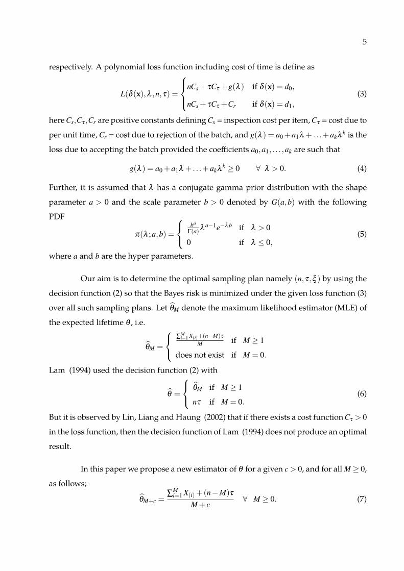
For non-polynomial loss function to obtain DSP, we consider the following values of coef-
ficients:
a0 = 2,a1 = 2,a2 = 2,Cr = 30,Cs = 0.5,Cτ = 0.5,ξ ∗ = 2,c∗ = 2.
and the results is given in Table 8.
Table 8: Minimum Bayes risk and corresponding optimal sampling plan for different val-
ues of a and b for DSP for non polynomial loss function
a b DSP
r(n0,τ0,ζ0,c0) n0 τ0 ξ0 c0
0.1 0.2 6.6966 2 0.6125 0.2250 1.6750
1.0 0.2 26.1494 3 1.0875 0.3750 1.1500
1.5 0.8 19.4142 4 0.9000 0.3750 0.0750
2.5 0.8 27.5525 4 1.0625 0.3750 1.0875
3.0 0.8 29.6926 2 1.0750 0.3500 1.8250
6.2.4 Comparison of DSP and LSP for Type-I Hybrid censoring under quadratic loss
function
In this section, the numerical comparison between DSP and LSP is given for Type-I hybrid
censoring. The values of coefficient a0 = 2,a1 = 2,a2 = 2,Cs = 0.5,rs = 0.3,Cτ = 5.0 and
Cr = 30 are used for comparison. Table 9-10 represent the numerical results of compari-
son. The Bayes risk of LSP includes a complicated integrals which is computed by simu-

24
lation techniques so Bayes risk of LSP is an approximation of exact Bayes risk of Bayesian
sampling plan.
Table 9: Minimum Bayes risk and corresponding optimal DSP
a b LSP 1 DSP
r(nB,rB,τB,δB) r(n0,τ0,ξ0,c0) n0 r0 τ0 ζ0 c0
2.5 0.8 26.0319 26.0338 6 3 0.2000 0.2750 0.6600
2.5 1.0 22.6430 22.6437 5 3 0.1875 0.2625 0.0725
3.0 0.8 29.7131 28.7890 4 2 0.2375 0.4250 0.0075
Cτ
0 24.6354 24.6736 4 4 0.8500 0.3000 0.3725
8 26.4662 26.4672 7 3 0.1625 0.2750 0.6600
16 27.2513 27.2513 7 2 0.1000 0.2875 0.5775
Table 10: Minimum Bayes risk and corresponding optimal DSP
LSP 1 DSP
Cs r(nB, ,rB,τB,δB) r(n0,τ0,ξ0,c0) n0 r0 τ0 ζ0 c0
0.5 26.0319 26.0338 6 3 0.2000 0.2750 0.6600
0.6 26.5578 26.5626 5 3 0.2500 0.2750 0.6600
0.7 26.9106 26.9114 3 2 0.2750 0.3125 0.2400
Cr
25 23.3583 23.3581 4 2 0.2375 0.3750 0.3350
30 26.0319 26.0338 6 3 0.2000 0.2750 0.6600
40 30.0072 30.0071 7 4 0.1750 0.2375 0.1075
Hence, for Hybrid Type-I censoring also the DSP is as good as LSP in terms of
Bayes risk.
1Bayes risk of LSP is obtain by simulation.

25
7 Conclusion
In this paper we have worked on the improvement of the paper of Lam (1994) where he
had used the MLE of the mean lifetime, which may not exist always for a Type-1 censored
sample. In fact Lin, Liang and Haung (2002) showed that the sampling plan proposed
by Lam (1994) is neither optimal, nor Bayes. The Bayesian sampling plan LSP proposed
by Lin, Liang and Haung (2002) provides a smaller Bayes risks than the sampling plan
provided by Lam (1994). Lin, Liang and Haung (2002) implemented the LSP for quadratic
loss function. It is observed that in case of higher degree polynomial loss function or
for a more general non-polynomial loss function LSP may not be very easy to obtain. In
this paper we have proposed a new decision theoretic sampling plan DSP based on an
estimator which always exists and showed that it is as good as Bayesian sampling plan LSP
in the sense that it minimizes the Bayes risk. It may be mentioned that although in this
paper we have considered Type-I censored sample only but the method can be extended
for other censoring cases also. More work is needed along that direction.
8 Acknowledgements
We express our sincere thanks to the referees and the editor for their useful suggestions
which led to an improvement over an earlier version of this manuscript.
Appendix
To prove (10) first we show that

26
r(n,τ,ξ ,c) = nCs + τCτ +a0 +a1µ1 +a2µ2 +2
∑l=0
Cl
ba
Γ(a)
∫ ∞
0λ a+l−1e−λbP(θM+c < ξ )dλ , (21)
Proof of (21)
r(n,τ,ξ ,c) = E{
L(δ (x),λ ,n,τ)}
= Eλ EX/λ
{L(δ (x),λ ,n,τ)
}
= Eλ
{(nCs + τCτ +a0 +a1λ +a2λ 2)P(θM+c ≥ ξ )
+(nCs + τCτ +Cr)P(θM+c < ξ )}
= nCs + τCτ +a0 +a1µ1 +a2µ2
+Eλ
{(Cr −a0 −a1λ −a2λ 2)P(θM+c < ξ )
}
= nCs + τCτ +a0 +a1µ1 +a2µ2
+∫ ∞
0(Cr −a0 −a1λ −a2λ 2)
ba
Γ(a)λ a−1e−λbP(θM+c < ξ ) dλ
= nCs + τCτ +a0 +a1µ1 +a2µ2 +2
∑l=0
Cl
ba
Γ(a)
∫ ∞
0λ a+l−1e−λbP(θM+c < ξ )dλ .
Proof of (10)
Using (8) in (21) we get∫ ∞
0λ a+l−1e−λbP(θM+c < ξ ) dλ
=∫ ∞
0λ a+l−1e−λb pS(ξ ) dλ +
∫ ∞
0λ a+l−1e−λb(1− p)H(ξ ) dλ
=∫ ∞
0λ a+l−1e−λbe−nλτ I( nτ
c <ξ ) dλ +n
∑m=1
m
∑j=0
(n
m
)(m
j
)(−1) j
×∫ ∞
0
∫ ξ
0λ a+l−1e−λ{b+τ(n−m+ j)}π
(x− τ j;m,c;m,λ (m+ c)
)dx dλ
=Γ(a+ l)
(b+nτ)(a+l)I( nτ
c <ξ )+n
∑m=1
m
∑j=0
(n
m
)(m
j
)(−1) j
×∫ ∞
0
∫ ξ
0λ a+l−1e−λ{b+τ(n−m+ j)}π
(x− τ j;m,c;m,λ (m+ c)
)dx dλ
=Γ(a+ l)
(b+nτ)(a+l)I( nτ
c <ξ )+n
∑m=1
m
∑j=0
(n
m
)(m
j
)(−1) j (m+ c)m
Γ(m)

27
×∫ ∞
0
∫ ξ
τ j;m,c
λ a+l+m−1e−λ{b+(m+c)x}(x− τ j;m,c
)m−1dx dλ
=Γ(a+ l)
(b+nτ)(a+l)I( nτ
c <ξ )+n
∑m=1
m
∑j=0
(n
m
)(m
j
)(−1) j (m+ c)m
Γ(m)
×∫ ξ
τ j;m,c
(x− τ j;m,c
)m−1Γ(a+ l +m)
{b+(m+ c)x}a+l+mdx
=Γ(a+ l)
(b+nτ)(a+l)I( nτ
c <ξ )+n
∑m=1
m
∑j=0
(n
m
)(m
j
)(−1) j (m+ c)m
Γ(m)
×∫ ξ−τ j;m,c
0
ym−1Γ(a+ l +m)
{b+(m+ c)τ j;m,c +(m+ c)y}a+l+mdy. (22)
Using C j,m = b+(m+ c)τ j;m,c in (22), we can write
n
∑m=1
m
∑j=0
(n
m
)(m
j
)(−1) j (m+ c)m
Γ(m)
Γ(a+ l +m)
Ca+l+mj,m
∫ ξ−τ j;m,c
0
ym−1
(1+ (m+c)y
C j,m
)a+l+mdy
=n
∑m=1
m
∑j=0
(n
m
)(m
j
)(−1) j Γ(a+ l)
(C j,m)a+l
Γ(a+ l +m)
Γ(m)Γ(a+ l)
∫ (m+c)(ξ−τ j;m,c)
C j,m
0
zm−1
(1+ z)a+l+mdz. (23)
Now taking a transformation z = u/(1−u), we have∫ C∗
j,m,c
0
zm−1
(1+ z)a+l+mdz =
∫ S∗j,m,c
0um−1(1−u)a+l−1du = BS∗j,m,c
(m,a+ l),
where C∗j,m,c =
(m+ c)(ξ − τ j;m,c)
C j,m, S∗j,m,c =
C∗j,m,c
1+C∗j,m,c
, and
Bx(α,β ) =∫ x
0uα−1(1−u)β−1du, 0 ≤ x ≤ 1,
is the incomplete beta function. Let us denote the cumulative distribution function of beta
by
Ix(α,β ) = Bx(α,β )/B(α,β ).
Then using (23), (10) is finally obtained as
r(n,τ,ξ ,c) = nCs + τCτ +a0 +a1µ1 +a2µ2 +2
∑l=0
Cl
ba
Γ(a)
[Γ(a+ l)
(b+nτ)(a+l)I( nτ
c <ξ )
+n
∑m=1
m
∑j=0
(−1) j
(n
m
)(m
j
)Γ(a+ l)
(C j,m)a+lIS∗j,m,c
(m,a+ l)
]. (24)
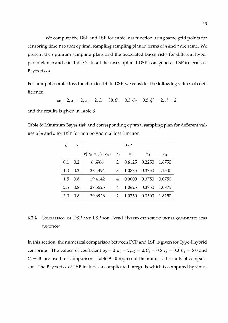
Proof of Result 3.1
28
Proof. Note that the Bayes risk is given by
r(n,τ,ξ ,c) = Eλ
{(nCs + τCτ +a0 +a1λ + . . .+akλ k)P(θM+c ≥ ξ )
+(nCs + τCτ +Cr)P(θM+c < ξ )}
= nCs + τCτ +Eλ
{(a0 +a1λ + . . .+akλ k)P(θM+c ≥ ξ )
+CrP(θM+c < ξ )}.
Now we know that a0+a1λ + . . .+akλ k ≥ 0 and Cr, the rejection cost, is non negative. Since
(n0,τ0,ξ0,c0) is the optimal sampling plan so the corresponding Bayes risk is
r(n0,τ0,ξ0,c0)≥ n0Cs + τ0Cτ . (25)
Now when ξ = 0 we accept the batch without sampling and the corresponding Bayes risk
is given by
r(0,0,0,0) = a0 +a1µ1 + . . .+akµk.
When ξ = ∞ we reject the batch without sampling and corresponding Bayes risk is given
by
r(0,0,∞,0) =Cr.
Then the optimal Bayes risk is
r(n0,τ0,ξ0,c0)≤ min{
r(0,0,∞,0),r(0,0,0,0),r(n,τ,ξ0(n,τ),c0(n,τ))}. (26)
Hence from equations (25) and (26) we have
n0Cs + τ0Cτ ≤ min{
r(0,0,∞,0),r(0,0,0,0),r(n,τ,ξ0(n,τ),c0(n,τ))},
from where it follows that
n0 ≤ min
{Cr
Cs
,a0 +a1µ1 + . . .+akµk
Cs
,r(n,τ,ξ0(n,τ),c0(n,τ))
Cs
}
τ0 ≤ min
{Cr
Cτ,a0 +a1µ1 + . . .+akµk
Cτ,r(n,τ,ξ0(n,τ),c0(n,τ))
Cτ
}.

29
References
Chen, L. S., Yang, M. C. and Liang, T. C. (2015), “Bayesian sampling plans for exponential distri-
butions with interval censored samples”, Naval Research Logistics, vol. 62, 604–616.
Childs, A., Chandrasekhar, B., Balakrishnan, N. and Kundu, D. (2003), “Exact likelihood inference
based on Type-I and Type-II hybrid censored samples from the exponential distribution”, Annals
of the Institute of Statistical Mathematics, vol. 55, 319–330.
Cramer, E. and N. Balakrishnan (2013). “ On some exact distributional results based on Type-I
progressively hybrid censored data from exponential distribution”, Statistical Methodology, vol.
10, 128-150.
Fertig, K. W. and Mann, N. R. (1974), “A decision-theoretic approach to defining variables sampling
plans for finite lots: single sampling for Exponential and Gaussian processes”, Journal of the
American Statistical Association, vol. 69, 665–671.
Gupta, R.D. and Kundu, D. (1998), “Hybrid censoring schemes with exponential failure distribu-
tion.”, Communications in Statistics - Theory and Methods, vol. 27, 3065 - 3088.
Grony, J. and E. Cramer (2017). “ From B-spline representations to gamma representation in hybrid
censoring”, Statistical Papers. DOI: 10.1007/s00362-016-0866-4. (To appear).
Hald, A. (1967) “Asymptotic properties of Bayesian single sampling plans”, Journal of the Royal
Statistical Society, Ser. B, vol. 29, 162–173.
Herstein, I. N. (1975) “Topics in Algebra,” John Wiley & Sons, New York.
Huang, W. T. and Lin, Y. P. (2002), “An improved Bayesian sampling plan for exponential popula-
tion with Type I censoring”, Communications in Statistics - Theory and Methods vol. 31, 2003–2025.
Lam, Y. (1988), “Bayesian approach to single variable sampling plans”, Biometrika, vol. 75, 387–391.
Lam, Y. (1990), “An optimal single variable sampling plan with censoring”, The Statistician, vol. 39,
53–66.
Lam, Y. (1994), “Bayesian variable sampling plans for the exponential distribution with Type-I cen-
soring”, The Annals of Statistics, vol. 22, 696–711.

30
Lam, Y. and Choy, S. (1995), “Bayesian variable sampling plans for the exponential distribution
with uniformly distributed random censoring”, Journal of Statistical Planning and Inference, vol.
47, 277–293.
Liang, T. C. and Yang, M. C. (2013), “Optimal Bayesian sampling plans for exponential distributions
based on hybrid censored samples”, Journal of Statistical Computation and Simulation, vol. 83, 922–
940.
Lin, C. T., Huang, Y. and Balakrishnan, N. (2008a), “Exact Bayesian variable sampling plans for the
exponential distribution based on Type-I and Type-II hybrid censored samples”, Communications
in Statistics - Simulation and Computation, vol. 37, 1101–1116.
Lin, C. T., Huang, Y. L., Balakrishnan, N. (2008b) “Exact Bayesian variable sampling plans for ex-
ponential distribution under type-I censoring”, In: Huber, C., Limnios, N, Mesbah, M., Nikulin,
M., eds., Mathematical methods in survival analysis, reliability and quality of life, pp: 151–162, Appl.
Stoch. Methods Ser., ISTE, London.
Lin, C., Huang, Y. and Balakrishnan, N. (2011), “Exact Bayesian variable sampling plans for the
exponential distribution with progressive hybrid censoring”, Journal of Statistical Computation
and Simulation, vol. 81, 873 - 882.
Lin, Y.P., Liang, T. C. and Huang, W. T. (2002), “Bayesian sampling plans for exponential distri-
bution based on type-I censoring data”, Annals of the Institute of Statistical Mathematics, vol. 54,
100–113.
Thyregod, P. (1975), “Bayesian single sampling plans for life-testing with truncation of the number
of failures”, Scandinavian Journal of Statistics, 61–70.
Tsai, T.R., Chiang, J.Y., Liang, T. , Yang, M.C.(2014), “Efficient Bayesian sampling plans for exponen-
tial distributions with type-I censored samples”, Journal of Statistical Computation and Simulation,
vol. 84, 964–981.
Wetherill, G. B. and Kollerstrom, J. (1979), “Sampling inspection simplified”, Journal of the Royal
Statistical Society, Ser. A, vol. 142, 1–32.