A New Constant Market Share Competitiveness Indexeinspem.upm.edu.my/journal/fullpaper/vol12no1/1. aishanudin.pdf · A New Constant Market Share Competitiveness Index Aisha Nuddin,

Malaysian Journal of Mathematical Sciences 12(1): 1–23 (2018)

MALAYSIAN JOURNAL OF MATHEMATICAL SCIENCES

Journal homepage: http://einspem.upm.edu.my/journal

A New Constant Market Share CompetitivenessIndex

Aisha Nuddin, A. J ∗1, Azhar, A. K. M.2, Gan, V. B. Y 3, andKhalifah, N. A. 4

1,2Institute for Mathematical Research, Universiti Putra Malaysia,Malaysia

1Department of Mathematics, Universiti Teknologi Mara, Malaysia2,3Graduate School of Management, IKDPN, Universiti Putra

Malaysia, Malaysia4School of Economics, Faculty of Economics and Management,

Universiti Kebangsaan Malaysia, Malaysia

E-mail:[email protected]∗ Corresponding author

Received: 16 May 2017Accepted: 15 August 2017

ABSTRACT

Constant-market-share analysis (CMSA) is one of the most widely em-ployed descriptive tool for measuring the export competitiveness of acountry relative to other countries or regions of trade for goods and ser-vices. Typically, export growth is attributed to growth in the country’sexport competitiveness and also to the growth effect of the market itself.However, CMSA measurement is prone to a number of methodologicalshort comings which stems from the CMS identities used in the analy-sis. Namely, the discrete approximation of continuously changing tradepatterns, the interaction effects term residual from the CMS identity de-composition and the arbitrary choice of weights attached to base periods.This paper addresses some of the short comings of the classic CMSA ap-

Aisha Nuddin, A. J et al.

proach. Within a geometric framework we reexamine the CMS decom-position and propose a new net-share approach that is easier to imple-ment and interpret. For researchers and policy makers, this methodologypresents a simpler but more consistent measurement for more accurateCMS measurement and interpretations of changing trade patterns.

Keywords: Constant Market Share analysis, competitiveness index, ex-port competitiveness.

2 Malaysian Journal of Mathematical Sciences

A New Constant Market Share Competitiveness Index

1. Introduction

In an increasingly globalised world in which there been a proliferation ofregional trading agreements, it is increasingly important to be able to under-stand and document changing trade patterns and how this reflects changes ina country’s competitiveness. Constant-market-share (CMS) analysis has longbeen used to analyse the export competitiveness of a country and has beenused to measure competitiveness relative to the rest of the world or within aspecific grouping of countries or well defined regional trading bloc such as theEuropean Union (EU) or the North American Free Trade Area (NAFTA). Putsimply, CMS analysis decomposes a country’s export growth into a compet-itiveness effect (CE) and the total growth effect (GE). The competitivenesseffect is defined as the increase in the quantity of a country’s exports due tothe increase in the country market share only (with global or regional exportsremaining constant). The total export growth effect is defined as the increasein the quantity of a country’s exports that are due to an increase in global orregional market share only (country exports share remaining constant).

CMS analysis was first introduced in the context of international trade byTyszynski (1951) then applied to regional economics by Perloff et al. (1960) whoused the term shift-share analysis. The technique’s popularity in analysing re-gional economic performance is credited to Lowell D. Ashby who introducedit to government policymakers (Ashby, 1964). Shift-share analysis focuses onregional economic growth driven by employment growth decomposes this em-ployment growth into several effects which is claimed to explain these regionaldisparities. The structural effect or growth effect which is also called the in-dustry mix effect due to the structure of regional employment was the firstdecomposition (Dunmore, 1986 and Esteban-Marquillas, 1972). This was fur-ther expanded to include the competitiveness effect and the allocation effectwhich resulted from a residual term from the shift-share accounting identi-ties (Esteban-Marquillas, 1972). Essentially, it seeks to understand the driversof growth between different economic regions. Shift-share analysis was thenextended to include new net change and net relative change identities to ac-count for the dynamic nature of economic growth (Herzog and Olsen, 1977and Kalbacher, 1979). The CMS methodology of analysis remains importantand relevant today as shown by Artige and Neuss (2014) who propose a newshift-share decomposition that addresses shortcomings of traditional shift-shareanalysis. There is another approach to CMS as introduced by Fagerberg andSollie (1987). Instead of decomposing the absolute change in exports they de-composes the change in market share into two static components, the producteffect and market effects and three dynamic components, the competitivenesseffect, the product (or commodity) adaptation effect and the geographical (or

Malaysian Journal of Mathematical Sciences 3


market) adaptation effect.

Shift-share analysis gradually expanded to explain patterns of internationaltrade competitiveness and become known as CMS analysis that focuses onexport shares of a focus country relative to the world. Applications of CMSanalysis include Lombaerde and Verbeke (1989) in a study of internationalseaport competition, Leamer and Stern (1970) in a study of international mar-keting and international trade and Hoen and Leeuwen (1991) who used CMS toexamine competitiveness in manufacturing trade of Eastern Europe. In similarstudies, Skriner (2009) and Rahmaddi and Ichihashi (2012) used CMS to assessthe performance of Austrian and Indonesian manufacturing exporters respec-tively. Jimenez and Martin (2010) used CMS to analyse the European exportmarket shares for the period 1994-2007. Finally, Bonanno (2016) presents someapplications of CMS to the Italian case.

However, CMS analysis being grounded on shift-share analysis, unfortu-nately shares its shortcomings as well. The chief problem is well known as the“CMS index number problem”. The problem stems from the fact that both acountry and world exports are changing continuously in time while CMS iden-tities are merely discrete time approximations. This makes the decompositionof growth and competitiveness effects inconsistent. Numerous authors have at-tempted to provide the best discrete time CMS decomposition to account forthe growth and competitiveness effects (Baldwin, 1958, Svennilson, 1954 andTyszynski, 1951). These efforts however create an additional problem where anew “residual or interaction term” is created from these decompositions (Mi-lana, 1988, Richardson, 1971). This interaction term was thought to be theinteraction between the structural or growth and competitive change (Baldwin,1958). But, it can also be thought of as measuring the growth of the coun-try’s export shares in rapidly expanding commodities and markets (Richardson,1971). Hence, it is not subject to easy interpretation. Furthermore, similar toshift-share analysis, the researcher has to make an arbitrary choice. For CMSanalysis, this relates to the choice of the base period of measurement whichbecomes the basis of weights to compute the structural and competitivenesseffects. This arbitrary choice in turn leads to the appearance of the interactionterm which one would hope to avoid.

The objective of this paper is to demonstrate how CMS can be reinterpretedusing a simple geometric approach which might help overcome the “unsolvable”index number inconsistency problem. This leads us to the construction of anew index that we call the Constant-Market-Share Competitiveness (CMSC)index which we believe is able to capture the competitiveness performance of acountry’s exports relative to others which can be global or relative to a specific



regional market. Our new index is motivated by the net relative change shift-share identities. We contribute by adapting the net relative change method todesign a new net share approach to CMS analysis which does not create theinteraction term. This will provide us a new solution that is easy to apply,understand and interpret. Our solution will be invaluable to the large numberof academics and policymakers that want to illustrate changing patterns ofcompetitiveness for countries or sectors both regionally and globally.

The remainder of the paper is organised as follows. Section 2 presentsthe basic CMS model and discusses the currently perceived problems withinthe existing CMS approach used in the literature. In Section 3 we presentour geometric framework before we outline our proposed measure of exportcompetitiveness derived from the results from Section 2. Section 4 presentsa numerical example to demonstrate the applicability of our approach andSection 5 concludes.

2. The Basic CMS Model

It is useful to begin with a description of the basic CMS model and tooutline the five key identities associated with CMS and described originally inRichardson (1971). Assume we are looking at world trade and we are lookingat competitiveness from a home country perspective. Hence, let p = the totalvalue of home exports and Q = the total value of world exports (home plusforeign exports). Hence, the share of exports of the home country(s) to theworld exports is given by s = p

Q . The basic identity of the CMS can thereforebe represented by;

dp

dt= s

dQ

dt+Q

ds

dt(1)

Richardson (1971) points out that there is a problem with writing the CMSidentity in the form of Equation (1) because it refers to an infinitesimally shorttime period whereas CMS analysis is usually performed over a discrete timeperiod usually annual changes. To address this problem Richardson (1971)proposed a number of new CMS identities which take into account the discretetime issue.

These are given as follows where ∆ represents a change and the superscriptsrepresent the initial and subsequent time periods in total exports Q and theshare of exports s and α is a constant.



∆p = s0∆Q+Q1∆s (2)

∆p = s1∆Q+Q0∆s (3)

∆p = s0∆Q+Q0∆s+ ∆s∆Q (4)

∆p = (αs0 + (1− α)s1)∆Q+ (αQ1 + (1− α)Q0)∆s for 0 < α < 1 (5)

Despite the work of Richardson (1971) above, the use of CMS has continuedto attract criticism (Jepma, 1986, Milan, 1988 and Oldersma an Van Bergeijk,1993). One of the main sticking points is what is called in the literature as the“index number problem” which is a problem that is related to the choice of anappropriate base year when one wants to study export competitiveness.

One of the contributions of this paper is to show how our geometric frame-work together with Milana’s identity can be used to address this “index numberproblem” in particular highlighted by Richardson (1971) and Milana (1988).Flexibility for researchers in using any of the identities will result in inconsis-tency in the decomposition of identity (1), Q1∆s represents the CE and s0∆Qrepresents GE while identity (2), Q0∆s represents CE and s1∆Q representGE. Identity (3) decomposes ∆p into three parts separating the residual term∆s∆Q from CE and GE. In identity (1) the residual ∆s∆Q is considered partof CE while in identity (2) it is considered part of GE.

Figure 1 demonstrate the decomposition of identity (3) using the area ap-proach. In addition, although other authors suggest adjustments and exten-sions to the basic CMS methodology; these new identities instead led to furtherinconsistencies with the CMS analysis. The identity proposed by Milana (1988)helped in solving inconsistency caused by the residual ∆s∆Q. Milana identifiedthis inconsistency as the “index number problem of CMS analysis” or simplythe “CMS problem” and he demonstrated that identity (5) with α = 0.5 is themost accurate discrete-time approximation of which is the exact decompositionof total export change between period 0 and 1 (superscript t denotes period).

Setting identity (5) with α = 0.5 as proposed by Milana (1988) we will have;

∆p =1

2∆Q(s1 + s0) +

1

2∆s(Q1 +Q0) (6)

Equation (6) which we now address as Milana’s identity can also be obtainedby adding identities (2) and (3) which follow Richardson (1971) who proposedusing both identities to obtain improved results. This can be demonstratedgeometrically by decomposing ∆p into the sum of the areas of two trapeziums



Figure 1: Area interpretation of the CMS components.

in the s versus Q graph as shown in Figure 2. The best solution is to divide theresidual ∆s∆Q equally between the GE and CE which gives us the Milana’sidentity.

In this case, the area of the trapezium 12∆s(Q1 +Q0) represents the growth

effect (CE) while the area of the other trapezium given by 12∆Q(s1 + s0) rep-

resents the competitive effect (GE). Hence, we have the following formulation;

∆p =1

2∆Q(s1 + s0) +

1

2∆s(Q1 +Q0) = CE +GE (7)

This formulation will be used in the construction of our geometric frameworkfor CMS analysis in the next section.

3. A Geometric Framework for CMS Analysis

In this section we show how the CMS can possibly be translated into ageometric space. To do this we build on the original geometric framework ofAzhar and Elliot (2003) to develop what we now call a Constant Market ShareSpace (CMSS). This new CMSS framework allows the researcher to visualizechanges and differences in both the competitiveness effects and total growth



Figure 2: Area representation of Milana (1988)’s identity for ∆Q > 0 and ∆s > 0

effects between units of analysis (usually countries) and also between differenttime periods. The space in the CMSS can also be divided into several regionsin which each region exhibits similar competitiveness characteristics.

To illustrate the applicability of our approach, assume a hypothetical CMSstudy of exports for n countries for a given period of time. The CMSS is a two-dimensional space that can capture each and every competitiveness effect (CE)and total growth effect (GE) for each of n countries for a given period where theCE and GE can be positive, negative or zero. We depict the competitivenesseffects (CE) on the vertical axis (+/-CE) and the total growth effects (GE) onthe horizontal axis (+/-GE).

The result is a two-dimensional space which is a square box with four quad-rants. The lengths of the sides of the CMSS are given by twice the maximumof the largest absolute value of whichever is larger of the CE or GE for theperiod of study. Figure 3 presents a hypothetical CMSS.

For a given country in a given period the Competitiveness and GrowthEffects for any of the n countries in the period of analysis can be representedby a single coordinate point in the CMSS. In Figure 3, points N and M arecoordinates of two representative countries, one of which (N ) has a positive CE



and a positive GE while M has a fall in both CE and GE. Since the length of thevertical and horizontal axis are equal and each quadrant is a square it meansthat the positive and negative sides are equal in length with the maximumlength of the side given by the absolute value of whichever is larger of CE orGE. Using set notation, a CMSS for n countries can be written as;

CMSS = {(x, y)| − |max(CEt, GEt)| ≤ x ≤ max(CEt, GEt),

−|max(CEt, GEt)| ≤ y ≤ max(CEt, GEt),

t = 1, 2, 3, ...m} (8)

Figure 3: The Constant Market Share Space (CMSS).

This ensures that the CMSS is a square such that all values of CE andGE of the analysis are captured within the dimensions of the space. The axesare labelled in accordance with the Cartesian plane in which the centre is theorigin, (0, 0) represents the unique position where (CE, GE) = (0, 0). QuadrantI contain all positive CE and GE values and quadrant III contains all negativeCE and GE values. Quadrant II consists of positive CE and negative GEvalues while quadrant IV consists of negative CE and positive GE values. Thediagonal line BOC is an isocline where the CE and GE are equal.

All the points in which the CE is greater than the GE are in the triangleABC while points in which the CE is less than the GE are captured in the



triangle BCD. Therefore, we have the following;

Proposition 1. The sum of all the CEs of the countries in the region ofanalysis which are below the x-axis is equal to the negative sum of all the CEsof the countries in the analysis which are above the x-axis.

Proof:

Assume a hypothetical CMS study of exports for n countries for a givennumber of years. Let CEi be the competitive effect of country i and let∑kt=1 CEi be the sum of the CEs above the x-axis (which are all positive)

and let∑nt=1 CEi be the sum of all the CEs below the x-axis (which are all

negative). Given that the sum of all the CEs of the countries in a CMS analysisis equal to zero then;

n∑t=1

CEi = 0 impliesk∑t=1

CEi +

n∑t=k

CEi = 0,

hence

k∑t=1

CEi = −n∑t=k

CEi (9)

We now map the points in the CMSS where changes in p are equal. Thismeans we are mapping the locus of equi-∆p. From equation (7), GE = -CE+ ∆p. In the CMSS this can be represented by a straight line with a slopeof minus unity. Hence, the locus of equi-∆p are straight lines parallel to thediagonal AD of the CMSS as seen in Figure 4. For all of the locus of equi-∆p,its corresponding ∆p is the vertical intercept where; ∀∆pt > ∆pt−1 implies(CE +GE)t > (CE +GE)t−1 = ∆pt−1. Figure 4 also shows the directionof increasing ∆p isoclines within the CMSS. Using the CMSS and the simpleproofs from Section 3 we are able to develop a new measure of constant marketshare that addresses the concerns raised by previous research in this area.

3.1 The Constant Market Share Competitiveness Index:The Net Share Approach

The next stage is to use the CMSS geometric framework to help proposea new CMS based competitiveness index. The competitiveness of a coun-try’s exports is a rather ambiguous concept in the economic literature. Someeconomists consider it similar to the concept of comparative advantage althoughthis is not a view shared by all academic researchers (Krugman,1996). For ex-ample,a country may lose its competitiveness but still maintain its comparative



Figure 4: Total change in exports ∆p isoclines.

advantage (Dunmore, 1986).

CMS measurement attempts to quantify the extent to which a country iscompeting in export markets relative to other countries in a given region. Ascompetitiveness measures the performance of a country in terms of exportsfor a given period, the change in export share (either positive or negative)for a country can be considered as the competitiveness of the exports of thatcountry. This is consistent with Porter et al. (2007). who stated that the mostintuitive definition of competitiveness is a country’s share of world marketsfor its products. This makes competitiveness a zero sum game, because onecountry’s gain comes at the expense of others. Rosenfeld (1959) argued thatthe competitive effect should not be influenced by economic structure if weare to separate the growth of exports into a growth effect and a competitiveeffect. This view is shared by Artige and Neuss (2014) who presented a newshiftshare methodology which does not follow the basic identities of the traditionalCMS approach. In their approach they proposed a method that separatesthe competitive effect from any influence of economic structure by associatinga uniform distribution of sectors to sectoral growth rates. Their shift shareidentity decomposes the difference between national employment growth andregional employment growth into the structural and competitive effects relativeto the national average.



In this paper we follow the Milana’s identity in decomposing the changein exports of a country into the growth and competitive effects and proposea new competitiveness index that we call the CMSC index. We differentiatethis CMSC index from the competitiveness effect. The CMSC index measuresthe competitiveness of the export of a country relative to the countries withinthe analysis. Our CMSC index is based on changes in the market share ofacountry in a specific period. This index together with CE and GE will beanalysed using the CMSS in determining the extent of export performance ofa country in a region.

To develop our index, as before let p = the value of home exports, Q = thetotal value of regional exports (home plus foreign exports) and s = p

Q representthe export share of the home country. Let the export share of the home countryat the beginning of the analysing period be;

s0 =p0

Q0(10)

and the export share of the home country at the end of the analysing periodbe;

s1 =p1

Q1(11)

The change in the export share ∆s = s1−s0 measures the changes in exportshares of countries in a region for a given period. Therefore, the term ∆s canbe defined as the “net share” of the share of exports for the focus countryover the period of analysis from a defined base period. Thus, our approachto competitiveness measurement in the context of CMS analysis can be calledthe “net share approach” of CMS analysis similar to the “net relative change”measurement of shift-share analysis.

An increase in a country’s export share ∆s (change in export share)implies adecrease in the export share ∆s of its competitors which is equal to the increasein the home country’s market share. Although this is a zero sum game for anychange in export share, we assume that winners are those with a positive ∆sand the losers are those with negative ∆s (it is a draw when ∆s = 0). Given theproperties described above a new competitiveness index can be based simplyon the equation ∆s = s1 − s0 but bounded by twice the largest export sharevalue for any given country within the time periods analysed where time is onceagain indexed as t = 1, 2, 3, ...m. This gives us the new competitiveness indexwhich we call the CMSC index. The CMSC index is given as;

CMSS =s1 − s0

2max(s1m, s

0m)

(12)



With the use of our new CMSC index, the change in export share of acountry ∆s is bounded by -1 and 1 and the total of all ∆s of the competingcountries must be equal to zero. Note that ∆s exhibits proportionate scalingsince the rate of change of ∆s with respect to s0 is equal and opposite tothe rate ofchange of ∆s with respect to s1 as shown by the following partialderivatives where; δ∆sδs0 = 1 and δ∆s

δs1 = −1. To demonstrate how we move fromthis simple equation to an actionable index we first consider the locus of equalCMSC indices (equi-CMSC lines).

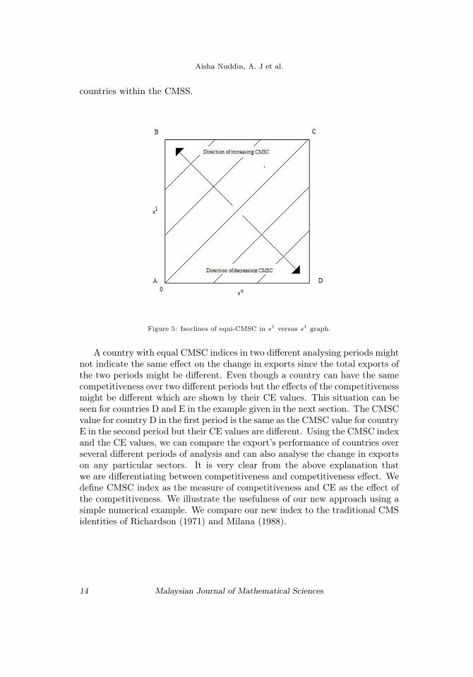
From ∆s = s1 − s0 we have s1 = ∆s + s0 which is a straight line in thegraph of s1 versus s1 with slope 1 and vertical intercept of ∆s. Hence,the locusof equi-∆s values are parallel lines to the main diagonal of the s1 versus s1

graph given in Figure 5. Note that ∆s is positive for s1 > s0 and is negativefor s1 < s0,thus it is positive above to the left of the diagonal AC and negativebelow (to the right of) the AC diagonal.

Finally, we consider the locus of equi-CMSC in the CMSS. From equation(7) the competitiveness effect is given by CE = 1

2∆s(Q1 +Q0), therefore;

∆s =2

Q1 +Q0CE (13)

As stated earlier we defined CMSS = s1−s02max(s1m,s

0m) ∝ ∆s. Since Q0 and

Q1 are constants and positive in the period of analysis, thus from equation(8) we have CMSC as a multiple of the CE and thus both are proportional toeach other respectively. Proportionality of CMSC and CE implies that locusof equi-CMSC are the same as the locus for equi-CE and hence, are horizontallines parallel to the x-axis as shown in figure 6. A CMSC index is positiveabove the horizontal axis and negative below.

Now that we have developed our new CMS index using a geometric ap-proach that allows us to capture all the changes in export market share for agiven period of time, we proceed to show its applicability in a simple numer-ical illustration. Since by definition CMSS capture all the CE and GE of thecountries in the region, the CE and GE values of any country in an analysingperiod is represented as a coordinate in CMSS. The position of the coordinatein CMSS together with its CMSC index value expresses the competitiveness ofthe country in the period. CMSC index expresses the competitiveness of ex-ports while CE expresses the effect of the competitiveness on the exports. Onthe other hand, GE reflects the change in exports due to growth (structural)effects. The CMSC index does not measure competitiveness relative to a baseperiod but it illustrates the competitiveness of a country relative to all of the



countries within the CMSS.

Figure 5: Isoclines of equi-CMSC in s1 versus s1 graph.

A country with equal CMSC indices in two different analysing periods mightnot indicate the same effect on the change in exports since the total exports ofthe two periods might be different. Even though a country can have the samecompetitiveness over two different periods but the effects of the competitivenessmight be different which are shown by their CE values. This situation can beseen for countries D and E in the example given in the next section. The CMSCvalue for country D in the first period is the same as the CMSC value for countryE in the second period but their CE values are different. Using the CMSC indexand the CE values, we can compare the export’s performance of countries overseveral different periods of analysis and can also analyse the change in exportson any particular sectors. It is very clear from the above explanation thatwe are differentiating between competitiveness and competitiveness effect. Wedefine CMSC index as the measure of competitiveness and CE as the effect ofthe competitiveness. We illustrate the usefulness of our new approach using asimple numerical example. We compare our new index to the traditional CMSidentities of Richardson (1971) and Milana (1988).



Figure 6: Competitiveness Index isoclines

4. Numerical Examples

In this section we provide a simple numerical example to show how themeasures of competitiveness can differ depending on the index used. We com-pare the interpretation of our numerical simulation to Milana’s CMS identityof equation (6) and the other traditional decompositions of equations (2), (3)and (4). The results are presented in Table 1. Assume there are five countriesin a hypothetical trading bloc. Column (1) shows the initial value of exports.Column (2) shows the change in exports in the following year (∆p). Totalexports are recorded in the final row of Table 1. The total of column (2) showsthat total trade expanded by 115 units from 800 to 915 units as shown in thetotal of column (3) that adds initial exports to the change in exports. Columns(4) and (5) measure the share of the country’s exports out of the total exportsin the first period (s0) and at the end of the second period (s1) respectively.By definition the addition of these shares must be equal to 1. Columns (8) and(9) represent CE and GE calculations based on Milana’s identity and Columns(10) to (14) are the traditional CMS identities from equations 2 to 4.

Our CMSC index is simply proportional to s1 − s0 and given that this isa zero sum game the total value of this unbounded index is zero as shown in



the final row of column (6). Furthermore, this desirable and logical propertyextends to the CMSC index itself as shown in the final row of column (7) inboth Table 1 and Table 2. In Table 1, the largest value of the share of exportis 0.4809 between these this period. For the next subsequent period in Table2, the largest share of export value is 0.4167. We use these largest values tobound the change in export share to calculate CMSC values in column (7) ofboth tables. Columns (10) and (11) disentangle the index into the CE and theGE respectively. The competitive effect is another zero sum game and mustsum to zero as shown by the final row of column (8) while the sum of the GEin column (9) must sum to the total expansion in trade which in this case is115 following from column(2).

The results for our hypothetical trading region can be presented in ourCMSS framework. These are shown in Figure 7. Generally, we find that inTable 1, our new CMSC index seems to be consistent with the traditional iden-tities. For instance, country A, B and C are shown to be increasing its exportcompetitiveness by CMSC values. This is reflected by CE values in column(8),(11),and (13) calculated from traditional CMS identities. All calculatedvalues indicate that countries A, B and C are becoming more competitive eventhough world export shares are increasing.

The ranking in exports competitiveness of the countries can be seen fromtheir position in the CMSS. The higher is its position, the higher is its compet-itiveness. Country A exports is the most competitive since its coordinate is inthe highest position in the CMSS. Country D is the least competitive since itis in the lowest position. The increase in exports for A is also the highest sincethe line parallel to the diagonal AD that passes through A is also the highest.Countries A, B and C have their CE higher than GE since these three coor-dinate are in triangle ADB where as countries D and E have their GE greaterthan CE since they are in triangle ACD.

In order to see the use of the competitive index in measuring the exportcompetitiveness between two different periods we simulate another hypotheticaltrading of the same five countries in Table 2 (A2 indicates second period analysisfor country A, etc.). Table 1 shows an example of increasing world exports butTable 2 shows an example where world exports are decreasing.

Looking at this single CMSS (Figure 8) we can analyse the performance ofany of the five countries exports in the first and the second period. In this casethe locus of equi-CMSC index is applicable only to countries within the sameperiod so there might be cases in which two countries from different periodwith the same CE but different CMSC index. This implies the two countries





Figure 7: CMSS of simulated data from Table 1

produce the same competitive effect but different competitiveness level withintheir period. Table 2 also reveals the inconsistencies of the traditional CMSidentities compared to our new index. For instance, the issue of inconsistentinterpretation appears in our example. Countries A2 and B2 are reported byCMSC values as becoming more competitive with increasing export shares. CEfigures of columns (8), (11) and (13) seem to agree but the interaction termis confusing and misleading with its negative figure. Furthermore, considercountries C2, D2 and E2 which is deemed to be indecreasing competitivenessby CMSC calculations but is again not consistent with the interaction termalthough it is consistent with traditional CE values. Tables 1 and 2 highlightthe usefulness of our new index. The researcher does not have to calculateall identities and the difficult to interpret interaction term does not appear.Thus, our new index does not presume a preferred or superior CMS identity,sparing the research of any philosophical entanglements. This is mainly amethodological argument where some authors like Richardson (1971) state thatthere is no a priori superiority of any identity while some like Milana (1988)suggest that equation (6) to be the closes discrete time approximation of thecontinuously changing export structure.

The same method can be used in analysing the performance of a countryexport over a period of several years. It can also be used in analysing the





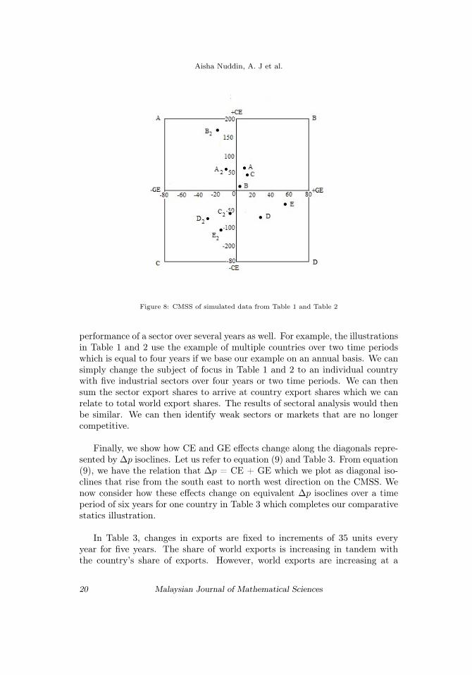
Figure 8: CMSS of simulated data from Table 1 and Table 2

performance of a sector over several years as well. For example, the illustrationsin Table 1 and 2 use the example of multiple countries over two time periodswhich is equal to four years if we base our example on an annual basis. We cansimply change the subject of focus in Table 1 and 2 to an individual countrywith five industrial sectors over four years or two time periods. We can thensum the sector export shares to arrive at country export shares which we canrelate to total world export shares. The results of sectoral analysis would thenbe similar. We can then identify weak sectors or markets that are no longercompetitive.

Finally, we show how CE and GE effects change along the diagonals repre-sented by ∆p isoclines. Let us refer to equation (9) and Table 3. From equation(9), we have the relation that ∆p = CE + GE which we plot as diagonal iso-clines that rise from the south east to north west direction on the CMSS. Wenow consider how these effects change on equivalent ∆p isoclines over a timeperiod of six years for one country in Table 3 which completes our comparativestatics illustration.

In Table 3, changes in exports are fixed to increments of 35 units everyyear for five years. The share of world exports is increasing in tandem withthe country’s share of exports. However, world exports are increasing at a



much faster pace than country exports. Unequivocally, CMSC values showthat the country’s exports are losing its international competitiveness. Onceagain, the advantage of CMSC in providing easy to interpret values is clear.CMSC is able to provide a quick guide to competitiveness without computingthe traditional CMS identities. Generally, CE figures provided by traditionalidentities and Milana’s identity agree with the CMSC that exports are losingits competitiveness. Nonetheless, let us consider CE values from t+ 4 to t+ 5.These CE values show a large disproportionate response to changes in theexport structure while CMSC values only show a small change from-0.02 to-0.09, a mere 0.07 units of change. Thus, while traditional CMS identities mayclassify this change as a large decrease of competitiveness, our CMSC indexwould instead present us with values that are proportional to changes in bothworld and country exports.

5. Conclusions

This paper presents a modest but useful geometric device for visualisingCMS analysis, named as the Constant Market Share Space, CMSS. The posi-tions of the coordinates representing the countries in CMSS give much infor-



mation about the countries competitiveness, competitiveness effects and thegrowth effects. We also introduced a new index as an indicator of the compet-itiveness of the exports of a country, CMSC which is based on the change ofthe export share within the period of analysis. Competitiveness of the exportsof a country (CMSC) is defined differently from its competitiveness effect(CE).These two measures are useful in analysing exports competitiveness across dif-ferent periods. Our approach is general and is applicable across products,sectors, or industries and for any number of years. This paper also exhibits theproposed geometric framework in tandem with Milana (1988) identity which isuseful in visualizing and solving the inconsistency in CMS analysis.

References

Artige, L. and Neuss, L. (2014). A new shift-share method. Growth and Change,45(4):667–683.

Ashby, L. D. (1964). The geographical redistribution of employment: an exam-ination of the elements of change. Survey of Current Business, 44(10):13–20.

Azhar, A. K. and Elliot, R. J. (2003). On the measurement of trade-inducedadjustment. Review of World Economics, 139(3):419–439.

Baldwin, R. E. (1958). The commodity composition of trade: selected industrialcountries, 1900-1954. The Review of Economics and Statistics, pages 50–68.

Bonanno, G. (2016). Constant market share analysis: A note. Economics andEconometrics Research Institute (EERI), Research Paper Series No 07/2016.

Dunmore, J. C. (1986). Competitiveness and comparative advantage of usagriculture. Increasing Understanding of Public Problems and Policies, pages21–34.

Esteban-Marquillas, J. M. (1972). A reinterpretation of shift-share analysis.Regional and Urban Economics, 2(3):249–255.

Fagerberg, J. and Sollie, G. (1987). The method of constant market shareanalysis revisited. Article in Applied Economics, 19(12):1571–1583.

Herzog, H. W. and Olsen, R. J. (1977). Shift-share analysis revisited: Theallocation effect and the stability of regional structure. Journal of RegionalScience, 17(3):441–454.

Hoen, H. W. and Leeuwen, E. H. V. (1991). Upgrading and relative competi-tiveness in manufacturing trade: Eastern europe versus the newly industri-alizing economies. Review of World Economics, 127(2):368–379.



Jepma, C. (1986). Extensions and application possibilities of the constant mar-ket shares analysis, the case of the developing countries’ export. Universityof Groningen.

Jimenez, N. and Martin, E. (2010). A constant market share analysis of theeuro area in the period 1994-2007. Economic Bulletin, (JAN.

Kalbacher, J. Z. (1979). Shift-share analysis: A modified approach. AgriculturalBusiness Research, 31(1):12–25.

Leamer, E. and Stern, R. (1970). Chapter 7: Constant market share analysisof export growth. Quantitative International Economics. USA: Allyn andBacon.

Lombaerde, P. D. and Verbeke, A. (1989). Assessing international seaportcompetition: a tool for strategic decision making. International Journal ofTransport Economics, 16(2):175–192.

Milana, C. (1988). Constant market sahare analysis and index number theory.European Journal of Political Economy, 4(4):453–478.

Oldersma, H. and Bergeijk, P. G. V. (1993). Not so constant! the constant-market-shares analysis and the exchange rate. De Economist, 141(3):380–401.

Perloff, H. S., DunnJr, E. S., Lampard, E. E., and Keith, R. (1960). Regions,resources,and economic growth. Baltimore: John Hopkins Press, USA.

Porter, M. E., Ketels, C., and Delgado, M. (2007). The microeconomic foun-dations of prosperity: findings from the business competitiveness index. TheGlobal Competitiveness Report, 2007-2008, pages 51–81.

Rahmaddi, R. and Ichihashi, M. (2012). How do export structure and compet-itiveness evolve since trade liberalization? an over view and assessmentof in-donesian manufacturing export performance. International Journal of Trade,Economics and Finance, 3(4):272.

Richardson, J. D. (1971). Constant-market-shares analysis of export growth.Journal of International Economics, 1(2):227–239.

Skriner, E. (2009). Competitiveness and specialisation of the austrian exportsector. a constant-market-shares analysis. Technical report, FIW WorkingPaper No.32.

Svennilson, I. and Unies, N. (1954). Growth and stagnation in the europeaneconomy. United Nations Economic Commission for Europe Geneva.

Tyszynski, H. (1951). World trade in manufactured commodities, 1899-1950.The Manchester School, 19(3):272–304.


Documents

A New Constant Market Share Competitiveness Indexeinspem.upm.edu.my/journal/fullpaper/vol12no1/1. aishanudin.pdf · A New Constant Market Share Competitiveness Index Aisha Nuddin,