A New Autoregressive Time Series Model Using

Laplace Variables

Kuttykrishnan A.P “Laplace autoregressive time series models”, Department of Statistics, University of Calicut, 2006

A New Autoregressive Time Series Model Using

Laplace ~ k r i a bles

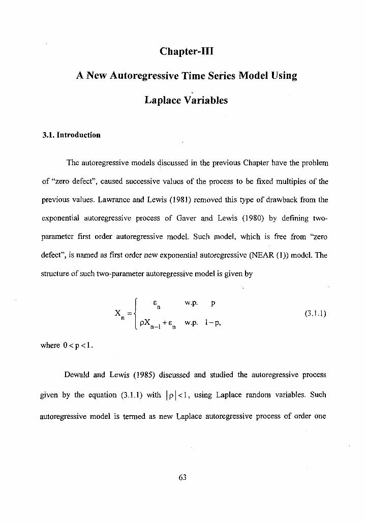
3.1. Introduction

The autoregressive models discussed in the previous Chapter have the problem

of "zero defect", caused successive values of the process to be fixed multiples of the

previous values. Lawrance and Lewis (1981) removed this type of drawback from the

exponential autoregressive process of Gaver and Lewis (1980) by defining two-

parameter first order autoregressive model. Such model, which is free from "zero

defect", is named as first order new exponential autoregressive (NEAR (1)) model. The

structure of such two-parameter autoregressive model is given by

where O < p < l .

Dewald and Lewis (1985) discussed and studied the autoregressive process

given by the equation (3.1.1) with 1 p l < l , using Laplace random variables. Such

autoregressive model is termed as new Laplace autoregressive process of order one

(NLAR (1)) and we can easily notice that the model is free from the "zero defect" with

the help of the following theorem.

Theorem 3.1.1.

Let (sn] be a sequence of independent and identically distributed random

variables given by

l-PZ where pl =

2 and Ln is a sequence of independently and identically distributed

1-P P 1

Laplace random variables. Then the relation (3.1.1) with X. - L(o) defines a

stationary autoregressive process with Laplace marginal distribution.

In the following Section we develop a new two-parameter autoregressive

process having structure (3.1.1) using asymmetric Laplace distribution.

3.2. A new autoregressive process using asymmetric Laplace variables

Since the asymmetric Laplace distribution is self-decomposable only if

0 l p C l , a two-parameter first order autoregressive process with the structure (3.1.1)

using asymmetric Laplace variables can be constructed by assuming the value of the

parameter p E [0,1). Hence we define a first order autoregressive process {X ) given

by (3.1.1) with O < p < l , O l p < l where ( E ~ ) is a sequence of independent and

identically distributed random variables selected in such a way that Xn is a stationary { l process with asymmetric Laplace marginal distribution.

Theorem 3.2.1.

The first order autoregressive process (3.1.1) with X. AL (p, 0) is stationary -

with asymmetric Laplace marginal distribution if and only if E, = U, +V, where Un

and Vn are two independent random variables with

and

where ( E ~ ~ } and ( E ~ ~ } are sequences of independent and identically distributed

, exponential random variables with means o / K and K o respectively.

Proof:

In terms of characteristic function, equation (3.1.1) becomes

If we assume ( x ~ } is stationary with asymmetric Laplace marginal distribution, then

(3.2.3) implies

2 1

( l - ~ ) , n , = ( l - p ) ( p + ( l ~ , " ~ $ ] and note that where n = p , n2=( l -p ) p+- 1 + ~

If Un and Vn are two independent random variables, then we can write

where

and

Conversely, if E, = U, + V, , where U and V given by (3.2.1) and (3.2.2) and n n

I f X dAL(p ,o ) thenwege tX d A L ( p , o ) . n-l - n =

Thus Xn is a stationary process with asymmetric Laplace marginal distribution. { 1 Hence the theorem.

We call the first order autoregressive process (xn) given by

where O < p < l and O < p < l with X dAL(p , c ) and c n = U n + V n , Un and V o = n

are two independent random variables defined in (3.2.1) and (3.2.2) as the new

asymmetric Laplace autoregressive process of first order ((NALAR (l)).

It may be noted that when p = 0, the NALAR (1) model is equivalent to the

ALAR (1) model.

Remark 3.2.1.

when^ = l (symmetric case), representation (3.2.1) and (3.2.2) reduces to the

form

0 w.p. p2 U n ={

Ln(o) w.p. l - p 2

and

where {L,(o)] is a sequence of symmetric Laplace random variables with

characteristic function (1.3.2). Hence, if X is stationary with symmetric Laplace { n l

marginal distribution then the innovation sequence {cn} of the model (3.1.1) can be

regarded as the sum of two independent random variables Un and Vn .

3.2.1. Properties of NALAR (1) process

From the representation (3.2.1) and (3.2.2), it is verified that

and

Hence

because cn = U +V . n . n

The conditional expectation

E(X n / X n-l = x ) = ( l - p ) p x + E ( ~ , )

That is, the conditional expectation E(Xn /Xn - l = X ) of the NALAR (1) process is

linear in X .

The autocorrelation function of the NALAR (1) process is obtained as follows:

Consider E(X n X n-l ) = E(E(X X / X = X)), n n-l n-l

2 whereE(XX / X =x)=( l -p )px +xE(cn) n n-l n-l

2 =(l-p)px +x ( l -p )p+ x p p p , using(3.2.4).

Hence

Therefore

E(X n X n-l ) = p 2 ( ~ + ( ~ - p ) p ) + ( l - p ) p 2 ~ 2 .

This implies

COV(X n X n-l ) = ( 1 - ~ ) ~ ( ~ ~ + 2 0 ~ )

Hence, the first order autocorrelation hnction of the NALAR (l) process is given by

Using similar arguments we can prove that the hth order autocorrelation function of the

process is given by

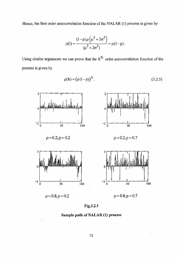
(3.2.5)

p = 0.8,~ = 0.2 p = 0 . 8 , ~ = 0.7

Fig.3.2.1

Sample path of NALAR (1) process

The simulated sample paths of NALAR (l) process for various model parameters p and

p when p = 0.5 and U = 2 are given in the above figures.

3.2.2. One parameter NALAR (1) model

In this Section we consider a tractable form of autoregressive model that is free

from "zero defect" using asymmetric Laplace distribution with structure similar to the

one-parameter TEAR (1) model discussed in Lawrance and Lewis (198 1).

Let X be an autoregressive process defined by { n l

where 0 < p < l and (E }is a sequence of independent and identically distributed

random variables. It may be noted that the model (3.2.6) has only one parameter p and

it is a particular case of (3.1.1) with p = l .

Pillai and Jose (1 994) established that the model given by the equation (3.2.6) is

defined if and only if stationary distribution of the process is geometrically infinitely

divisible. Since asymmetric Laplace distribution belongs to the class of geometrically

infinitely divisible distributions, it is possible to construct a stationary process {X,}

with structure given by (3.2.6) for the asymmetric Laplace distribution.

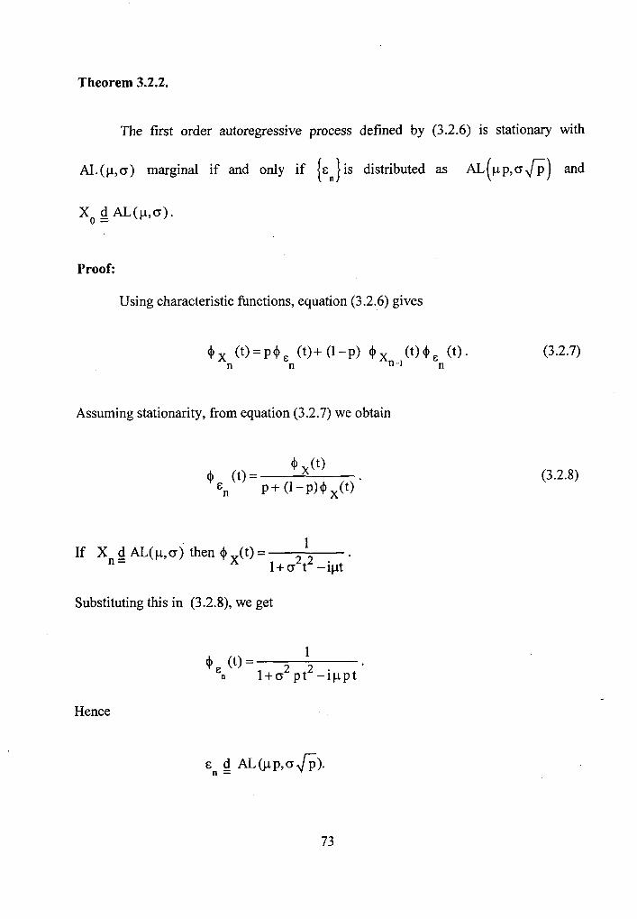
Theorem 3.2.2.

The first order autoregressive process defined by (3.2.6) is stationary with

AL (p ,o ) marginal if and only if {E } is distributed as A L ( ~ p,o h) and

Proof:

Using characteristic functions, equation (3.2.6) gives

Assuming stationarity, from equation (3.2.7) we obtain

If X d &(p, o ) then 0 X(t) = 1

n = I + 02t2 -ipt *

Substituting this in (3.2.8), we get

Hence

Conversely, if {E"} is a sequence of independent and identically distributed

AL (p p, o h) random variables and X d AL (p, o ) , then from (3.2.7), when n = l , 0 =

we have

If X dAL(p ,o) thenwegetX d AL(p ,o) . n-l = n =

Thus X is a stationary process with asymmetric Laplace marginal distribution. { I Hence the theorem. 0

We call the autoregressive process defined in (3.2.6) with X o = d AL(p,o) as the

TALAR (1) process.

From the definition (3.2.6) of the model it is easily verified that

Hence

1

$ (t) = P 4 & (t) , when n+m. n n l - ( l - ~ ) $ & ( 9

n

If X. has an arbitrary distribution and {&,}is a sequence of independent and

identically distributed random variables such that E d AL (p p,o&) then from n =

(3.2.10) we get

1 ox ('1 = 2 2 , when n+m. l + o t - i p t

Hence, if Xohas an arbitrary distribution then the autoregressive process is

asymptotically stationary with AL(p, o) marginal distribution.

When p = 1, the NALAR (1) model reduced to the TALAR (1) model. Hence,

for the TALAR ( l ) model, the regression of X on X is n n -l

E ( X / X = x ) = ( l - p ) x + p p . n n-l

th and the h order autocorrelation function p(h) is

The joint characteristic function of (X n-I ,X n )of the TALAR (1) process is

given by

1 l -P +X ,X (',S)= 2 2 + 2 2

n-l n I + o S - i p S 1 + o ( t+s ) - ip ( t+s ) 1 From the expression it is clear that 4 ( t,s) z (I ( S, t ) and hence the

n-1' n 'n-lyxn

process is not time reversible.

Construction of usual higher order autoregressive models of the form (1.1 . l )

using asymmetric Laplace distribution is a complicated problem. This is because it is a

difficult task to establish the distribution of innovation sequence {cn} so as to ensure

that {X,] is stationary with asymmetric marginal distribution if {xn] is given by

(1.1.1). Here we present a tractable form of higher order autoregressive model using

asymmetric Laplace distribution.

Let X be a an autoregressive process defined by { n l

X + E W.P. p1 n-l n

n

k where Cp. = 1 , 0 < p. < I , i = 0, l ,..., k and {\ ] is a sequence of independent and

i=O *

identically distributed random variables. Then X given by (3.2.12) defines a { n l

stationary autoregressive process of order k with X AL(p,o) if and only if {cn] is 0 -

distributed as (p P,, o 6) .

The sample path of TALAR (1) process for various values of p and p when

o = 1 is given in the following figures.

Sample path of TALAR (1) process.

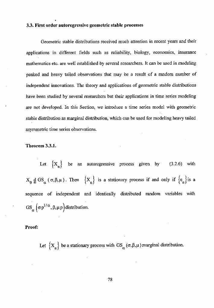
. 3.3. First order autoregressive geometric stable processes

Geometric stable distributions received much attention in recent years and their

applications in different fields such as reliability, biology, economics, insurance

mathematics etc. are well established by several researchers. It can be used in modeling

peaked and heavy tailed observations that may be a result of a random number of

independent innovations. The theory and applications of geometric stable distributions

have been studied by several researchers but their applications in time series modeling

are not developed. In this Section, we introduce a time series model with geometric

stable distribution as marginal distribution, which can be used for modeling heavy tailed

asymmetric time series observations.

Theorem 3.3.1.

Let (X,} be an autoregressive process given by (3.2.6) with

X. 4 - GS a (o ,P ,p) . Then {X,} is a stationary process if and only if {E,]~s a

sequence of independent and identically distributed random variables with

GS (a P, p p) distribution. a

Proof:

Let {X,] be a stationary process with GSa (a, P, p ) marginal distribution.

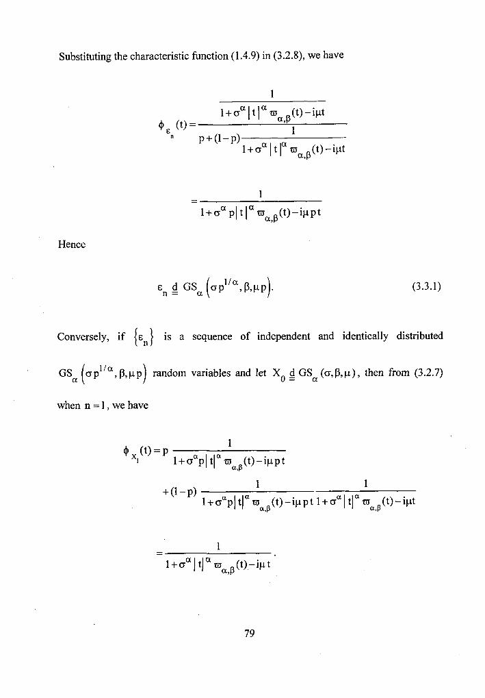
Substituting the characteristic function ( l .4.9) in (3.2.8), we have

Hence

Conversely, if {E,} is a sequence of independent and identically distributed

GS (o plia, P, p p) random variables and let X OSa (G, P,p), then from (3.2.7) a 0 -

when n = 1, we have

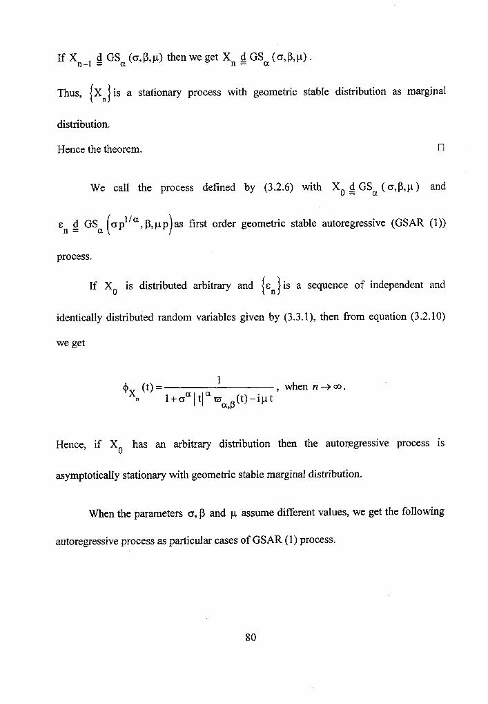
I f X n-l d G S - (q8 ,p) thenwegetX dGSa(o,P,p). a n =

Thus, { x ~ } is a stationary process with geometric stable distribution as marginal

distribution.

Hence the theorem.

We call the process defined by (3.2.6) with X 0 = d GSa (o ,P,p) and

E n - GS a (opl'a, j3,pp)as first order geometric stable autoregressive (GSAR (1))

process.

If X. is distributed arbitrary and {cn}is a sequence of independent and

identically distributed random variables given by (3.3.1), then from equation (3.2.10)

we get

4 ( 0 = 1 , when n + m .

1 + o a J tla m ( 0 - i p t a,P

Hence, if X. has an arbitrary distribution then the autoregressive process is

asymptotically stationary with geometric stable marginal distribution.

When the parameters o, P and p assume different values, we get the following

autoregressive process as particular cases of GSAR (1) process.

Case (i): Let o = 0 .

In this case the geometric stable distribution is reduced to exponential

1 distribution with characteristic function $(t) = - . Then the GSAR (1) process is

l - ip t

stationary with exponential marginal distribution. This model, known as TEAR (1)

model, is discussed in Lawrance and Lewis (1981).

Case (ii): Let a = 2 , p = 0.

In this case the geometric stable distribution is reduced to symmetric Laplace

distribution with characteristic function $(t) = 1 . Now the GSAR (1) process is

l + 0 2 t 2

stationary with symmetric Laplace distribution as marginal distribution if and only if

{cn} is a sequence of independent and identically distributed Laplace variables such that

E d p 1 ' 2 ~ n , where L is a sequence of symmetric Laplace variables. n = "1

Case (iii): Let a = 2, p # 0.

When a = 2 and p is any non-zero real number then the geometric stable

distribution is reduced to asymmetric Laplace distribution with characteristic function

1 ($(Q = . Then the GSAR (1) process is stationary with asymmetric

l + 0 2 t -ipt

Laplace distribution (AL (p,o)) if and only if {cn] is a sequence of independent and

identically distributed asymmetric Laplace random variables AL ( p p, o p l l 2 )

Case (iv): Let a E (0,2), p = 0 .

When a E (0,2) and p = 0 , then the geometric stable distribution is reduced to

the Linnik distribution with characteristic function $(t) = 1

(see Kozubowski l + o a l tla

and Rachev (1999)). Then the GSAR (1) process defines a first order stationary

autoregressive process with Linnik distribution as marginal distribution if and only if

{gn) is a sequence of independent and identically distributed Linnik variables such that

l/a L 'n g P a,n , where { L ~ , ~ ] is a sequence of Linnik random variables with

characteristic function +(t)-= 1

l+rra l tla

The model discussed in this case is similar to the past innovations process of Anderson

and Amold (1993). They studied different forms of autoregressive process with Linnik

distribution as marginal distribution and discussed their applications in modeling stock

price changes.

Case(v): Let p=O, O < a l l .

For p = 0 and 0 < a i l , the geometric stable distribution on (0, m) has the

I Laplace transform f (S) = S 2 0 (see Kozubowski and Rachev (1 999)). In this

l + o a s a '

case, the geometric stable distribution reduces to the Mittag-Leffler distribution

discussed in Pillai (1990 (b)). It is a generalization of exponential distribution, to which

it reduces for a = 1 (for more properties and applications of Mittag-Leffler distribution

see Pillai and Sabu George (1984), Jayakurnar and Pillai (1996), Weron and Kotulski

(1996) and Lin (1998, 2001)). Now the GSAR (1) process defines a stationary process

with Mittag-Leffler distribution as marginal if and only if is a sequence of

independent and identically distributed Mittag-LeMer variables, such that

E d Mn, where M is a sequence of Mittag-Leffler variables with Laplace n = ( "1

transform 1

l + o a s a

Jayakumar and Pillai (1993) introduced and studied first order autoregressive

process Xn = pXn-I + E,, 0 5 p < l , using semi Mittag-Leffler marginal distributions.

The semi-Mittag-Leffler distribution is a class of distribution defined on positive real

line with Laplace transform 1

where q(s) satisfies the fictional equation 1 +m

q(s) = a q(bs), 0 < b < 1 and a is the unique solution of a ba = 1, 0 5 a < 1. The Mittag-

Leffler distribution is a special case of semi Mittag-Leffler distribution. They

established that the first order autoregressive equation

defines a stationary process if and only if S M ~ ' s are semi Mittag-Leffler and with

X d S M . O = n

3.4. Tailed Laplace distribution and process

The concept of tailed distributions was introduced in Littlejohn (1994) while

discussing non-Gaussian time series models. Muralidharan (1999) considered tailed

distribution in the context of mixing a degenerate distribution (degenerate at zero) and a

continuous distribution such as exponential, Weibull, gamma etc. and discussed

inference problems related to such models. The tailed distributions are used as a model

in several situations where the variable can take either zero value with certain

probability or a random variable with remaining probability. Hence the tailed

distribution can be used as a model in different areas like dose response in the medical

field, flow of water in a river which is dry for a part of the year, economics that show

dull behavior in money circulation etc.

Definition 3.4.1.

Let X be a random variable with characteristic h c t i o n 4 x(t) . Then a random

variable Y with characteristic function

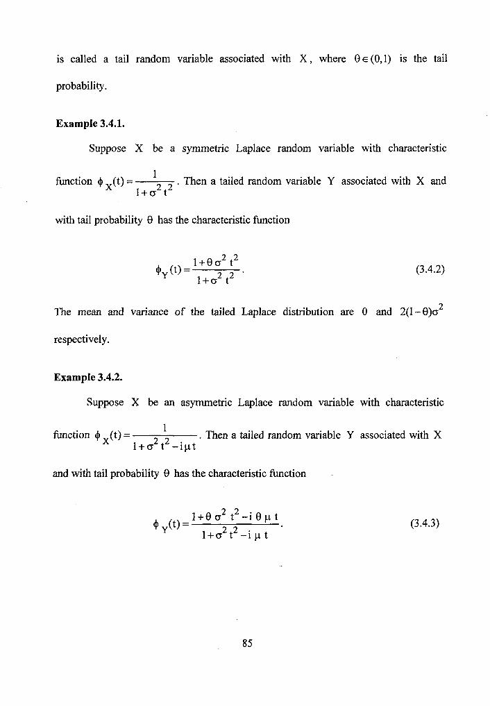
is called a tail random variable associated with X , where 8 E (0,l) is the tail

probability.

Example 3.4.1.

Suppose X be a symmetric Laplace random variable with characteristic

function 4 X(t) = 1 . Then a tailed random variable Y associated with X and

l + 0 2 t 2

with tail probability 8 has the characteristic function

The mean and variance of the tailed Laplace distribution are 0 and 2(1-0)~ 2

respectively.

Example 3.4.2.

Suppose X be an asymmetric Laplace random variable with characteristic

h c t i o n 9 x(t) = 1 . Then a tailed random variable Y associated with X

1+o2 t2 - ip t

and with tail probability 8 has the characteristic function

If Y is a random variable with characteristic function (3.4.3) then we represent it as

Y - d ALT(p, o,0) .

The mean and variance of the tailed asymmetric Laplace distribution are

p(1- 0) and p2 (l - e2) + 2(1- 0)02 respectively.

Now we develop an autoregressive model with tailed marginal distribution using

the model discussed in Lawrance and Lewis (1 98 1).

Theorem 3.4.1.

The first order autoregressive equation (3.2.6) defines a stationary first order

autoregressive process with tailed asymmetric Laplace marginal distribution if and only

if {E,} is a sequence of independent and identically distributed ALT py, o f i , 2) random variables with X d ALT(p, o, Q), where y = p + (1 -p)@ .

0 =

Proof:

Assume {X,} is stationary with tailed asymmetric Laplace distribution having

characteristic function (3.4.3). Then, from (3.2.8) using characteristic function we get

Simplifying, we get

l + 0 2 0 t2 - i p e t 0, (t) = 2 2 , where y=p+(l-p)8.

n l + o y t - i p y t

Hence

Conversely, if { E ~ ] is a sequence of independent and identically distributed

random variables and X d ALT ( p, o, B) , then from (3.2.7) when 0 =

I f X dALT(p,o,B)thenwegetX dALT(p,o,8) . n-l = n =

Thus {X"} is stationary with tailed asymmetric Laplace marginal distribution.

Hence the theorem.

We call the first order autoregressive process given by the structure (3.2.6) with

X d ALT (p, G, 0 ) and E d ALT as the fist order tailed asymmetric o = n =

Laplace autoregressive (ALTAR (1)) process.

If X. is distributed arbitrary and (E,) is a sequence of independent and

identically distributed ALT random variables then from (3.2.10) we get

2 2 1 + o 0 t -ip0t 4 (1) = , when n+m.

n 1 + d t 2 -ipt

Hence if X. has an arbitrary distribution then the autoregressive process is

asymptotically stationary with ALT(p, o, B) marginal distribution.

For the ALTAR ( l ) process (X"},

E(X n )=P(~-Q) ,

var(x ) = p2 (1 - e2) + 2(1- 0)02 n

and

Therefore, regression of X on X is linear (in X ) and given by n n -l

E(X / X =x)=( l -p ) X + p(y-8). n n-l

The covariance between Xn and Xn-h is obtained on considering the representation

(3.2.6) and simple computations show that

h COv(Xn ,X n-h ) =(l-p)Cov(X n-l , X n-h ) =(l-p) C O V ( X ~ _ ~ ,Xn-h ) .

Hence, the autocorrelation function of the ALTAR (l) process is given by

Note that p(h) is always positive i d so the variables are positively correlated.

It is easily verified that the joint characteristic function of (X n-l ,Xn) is not

symmetric in t and S . Hence the ALTAR (l) process is not time reversible.

3.5. A general first order autoregressive process

In this Section, we consider a general first order autoregressive model with three

parameters given by the structure

E n W-P PO

p x +E w.p p1 n-l n

pXn-I W.P P27

where po, pl and p2 are probabilities with p, + pl + p2 = 1 , 0 < p < l and {cn} is a

sequence of independent and identically distributed random variables.

The equation (3.5.1) have a direct physical interpretation as the observed process Xn at

time n , is one of three possibilities:

(i) with probability po, there is a scatter of values of Xn = en , independent of

X . n -l

(ii) with probability p,, Xn = p X + cn , and is always above or below the n-l

line X = p Xn-I . n

(iii) with probability p2, the values of Xn are in the line Xn = p X . n-l

When p2 = 0, we obtain the autoregressive model with structure (3. l . l ) and

when p. = p2 = 0, the model reduced to (2.2.1). Hence, this model is a general case of

(2.2.1) and (3.1.1).

The first order autoregressive model (3.5.1) can be expressed in the form of an

additive, linear, random coefficient autoregressive process as

=

where {(A,, I,), n t l} , is a sequence of independent and identically distributed discrete

random variables with distribution given by

Under stationary assumption and X, - c l , the characteristic function 4 x(t) of the

process { x ~ } is

WX(P t) $ =

p2 , where 0 = - . 1-(1-0)$,(~ t) l-P,

Hence, the stationary process {X,} given by the structure (3.5.1) is geometrically

infinitely divisible.

JevremoviC (1990) studied a first order autoregressive model with structure

(3.5.1) using mixed exponential marginal distributions and JevremoviC and MaliSiC

(1993) developed a moving average model similar to this structure using exponential

marginal distribution.

3.5.1. First order Laplace generalized autoregressive process

Here we develop a stationary process {X,) given by (3.5.1) using Laplace

marginal distribution. In the following Theorem, we show that that the innovation

sequence {E,) is a sequence of convex mixture of Laplace distributed random variables

so as to ensure X, is stationary with Laplace distribution as marginal distribution. 1 Theorem 3.5.1.

Let X d L ( o ) . Then the first order autoregressive equation given by (3.5.1) 0 =

defines a stationary autoregressive process with Laplace marginal distribution if and

only if innovations are of the form

where {L,} is a sequence of independent and identically distributed Laplace random

1-p2 variables with characteristic function (l .3.2) and 8 = 2

1 - ~ 2 - ~ PO

Proof:

Using characteristic functions, equation (3.5.1) gives

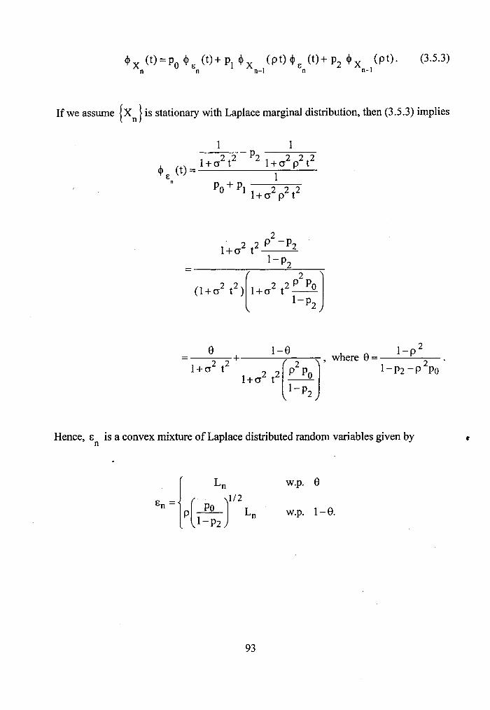
$ , ( t ) = p 0 ( t )+P,$. ( ~ t ) $ & ( t ) + P ~ $ , (P'). (3.5.3) n O &n n-I n n-I

If we assume (xn} is stationary with Laplace marginal distribution, then (3.5.3) implies

- - 0 1-8 1-p2 2 2 +

, where 8 = 2 - l + o t 1 - ~ 2 - ~ PO

Hence, cn is a convex mixture of Laplace distributed random variables given by ~t

Thus {E,} is a sequence of independent and identically distributed random variables

that has probability distribution, which can be generated as the (8,l- 8 ) mixture of

Laplace random variables.

Conversely, if E is a sequence of independent and identically distributed random { n l variables given by (3.5.2) and X d L ( o ) then from (3.5.3), when n = l , we have

0 =

I - p L where 8 =

2 - 1 - ~ 2 - P PO

Hence

Suppose X d ~ ' ( o ) , then it can be shown that X d L ( 0 ) . n-l = n =

Therefore, the process (3.5.1) is stationary with Laplace marginal distribution.

Hence the theorem.

L

Based on the above theorem, we can define first order Laplace general

autoregressive process (LGAR (1)) as follows:

Let X L ( o ) and for n = 1,2, ... 0 -

where O<po,pl,p2<1 with po+pl+p2,=1 , O < p < l and (E n }is a sequence of

independent and identically distributed convex mixture of Laplace random variables

defined in (3.5.2).

Remark 3.5.1.

It is easy to verify that

(i)if p2 > * then 8 < 0 and PO

(ii) if p ' < A then 8 > 1. 1-P,

In a situation like this the distribution of the innovation sequence is a mixture of

Laplace distribution with negative weights. JevremoviC (1991) demonstrated the use of

autoregressive process to simulate a sequence of values of the random variable whose

n

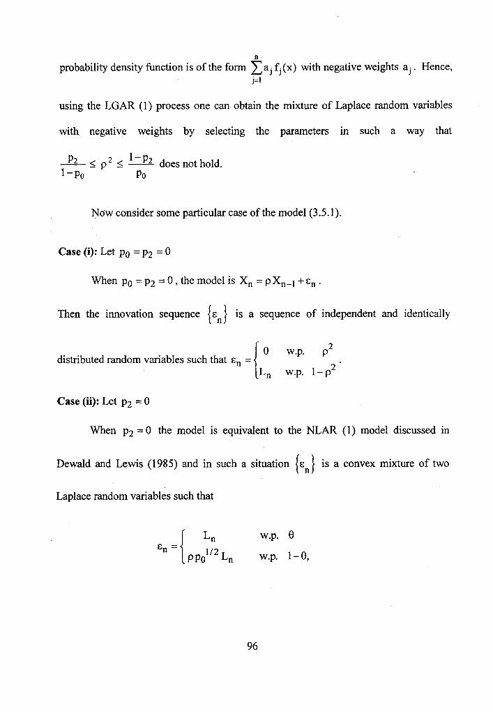
probability density function is of the form x a j f,(x) with negative weights a j . Hence, j=1

using the LGAR (1) process one can obtain the mixture of Laplace random variables

with negative weights by selecting the parameters in such a way that

p2 g p 5- - P2 does not hold. l-PO P0

Now consider some particular case of the model (3.5.1).

Case (i): Let p0 = p2 = 0

When p. = p2 = 0, the model is X, = pXn-l + En .

Then the innovation sequence {E,] is a sequence of independent and identically'

0 w.p. p2 distributed random variables such that E, =

L, w.p. l - p 2 '

Case (ii): Let p2 = 0

When p2 = 0 the model is equivalent to the NLAR (1) model discussed in

Dewald and Lewis (1985) and in such a situation E is a convex mixture of two { n l

Laplace random variables such that

1-pL where 0 =

1-p2 PO '

Case (iii): Let p = l

When p = l , the innovation sequence (E,] is an independent and identically

distributed sequence of scaled Laplace random variables L, provided

The autocorrelation function p (h ) of the LGAR (1) process is obtained as

follows:

Consider

E( X, xnVh ) = E(E( X, x ,-~ I x ~ - ~ = X )) ,

where

E( X, = X ) = p O xE(En)+pl (pE(Xn-1 Xn-h/Xn-h ))

= (p, +p2 ) p X E(X n-I ) , because E(E n ) = 0.

= ((p, + p2 ) p) h x2, by repeatedly using the procedure.

Hence

E( XnXn-h ) = ( P ( P I + P ~ ) ) ~ E(x2) .

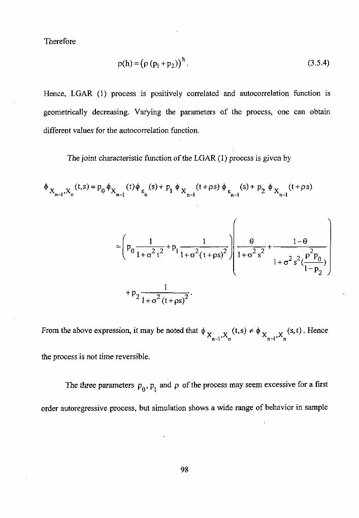
Therefore

Hence, LGAR (1) process is positively correlated and autocorrelation function is

geometrically decreasing. Vafying the parameters of the process, one can obtain

different values for the autocorrelation function.

The joint characteristic function of the LGAR (1) process is given by

4 (t9s)=p0Ox ( t ) O E ( s ) + p 4 ( t+ps )4 ( s ) + p 2 0 x ( t+ps) 'n-1"n n-l n I 'n-1 E n - ~ n-l

From the above expression, it may be noted that 4 (t,s) # 4 (S, t) . Hence 'n-I "n 'n-I "n

the process is not time reversible.

The three parameters po, pl and p of the process may seem excessive for a first

order autoregressive process, but simulation shows a wide range of behavior in sample

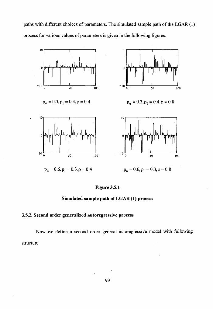
paths with different choices of parameters. The simulated sample path of the LGAR (1)

process for various values of parameters is given in the following figures.

Figure 3.5.1

Simulated sample path of LGAR (1) process

3.5.2. Second order generalized autoregressive process

Now we define a second order general autoregressive model with following

structure

2 P2+P4 (ii) 8 > l if p < 1-PO

Therefore, whenever the values of the parameters do not satisfy the condition

P2 +P4 6 p 5 , random variable E, is a mixture of Laplace random 1-PO P0

variables with negative weights. Hence using the stationary autoregressive process

(3.5.6) with p, = p2 =p and X d L ( o ) , one can obtain the mixture of Laplace 0 =

random variables with negative weights.

3.5.3. First order asymmetric Laplace generalized autoregressive process

Let {X,) be a stationary sequence of asymmetric Laplace random variables

given by the structure (3.5.1). Then the probability distribution for innovative sequence

(E,} is obtained by substituting 4 *(t) = 1

in (3.5.3). The solution is 1+02 t2 - i p t

much-complicated one, and to make the problem a simple one we consider the

following autoregressive model developed by MaliSiC (1 987).

Let {X,) be a sequence of random variables given by

I PEn W.P P,

X, = X + p&, w.p p* n-l

X n -l W-P P2

where O<p , p , p < l with po+p l+p2 = l , O < p < l and 0 1 2 (E,} is a sequence of

independent and identically distributed random variables.

Theorem 3.5.2.

Let X d AL (p, o ) . Then the first order autoregressive equation given by 0 =

(3.5.8) defines a stationary autoregressive process with asymmetric Laplace marginal

distribution if and only if innovations are of the form

Proof:

From equation (3.5.8), using the characteristic functions we have

4. ( t )=p0 4 , ( P O + P, 4. ( t ) 4, (PO+ P, 4, ( 9 . (3.5.9) n n n-l n n-l

If we assume Xn is stationary with asymmetric Laplace marginal distribution, then { l (3.5.9) implies

Hence

- - 1 -p2 2 2

l -p +o p t - i p p t 2 0 0

Conversely, if E is a sequence of independent and identically distributed asymmetric { n l

Laplace random variables given by (3.5.10) and X d AL (p, o ) then from (3.5.9), 0 =

when n = 1, we have

Suppose X d AL (p, G ) , then it can be shown that X d AL (p, o ) . n-l = n =

Therefore, the process (3.5.8) is stationary with asymmetric Laplace marginal

distribution if X d AL (p, o ) . 0 =

Hence the theorem.

The autocorrelation function p(h) of the mode1 (3.5.8) is obtained as follows:

Consider

E( X, X,-] ) = E(E( X, xnW1 I X,-] = X )) ,

where

= pox p + (pl + p2)x2 , because E(&,) = P (1-p2)p

Hence

c o w n ,X n-l )=(p ,+p2)(p2+2c2)

Therefore

In general, the autocorrelation function of the process (3.5.8) with asymmetric Laplace

h marginal distribution is given by p(h) = (p, + p2) .

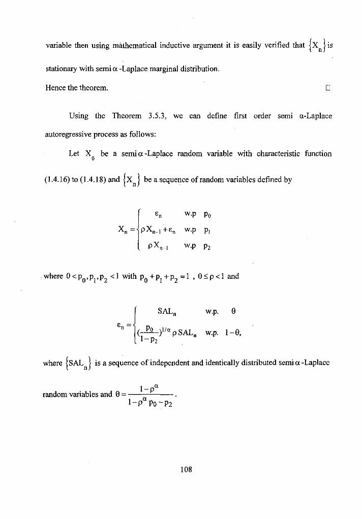
3.5.4. First order semi a-Laplace autoregressive process

Now we consider a stationary process using a generalized class of distributions,

namely semi a -Laplace distributions, defined in Pillai (1985). Let (xn} be a

stationary sequence with semi a -Laplace marginal distribution and with the structure

(3.5.1). Then from (3.5.1) the question is whether there is a valid probability

distribution for innovative sequence cn . { l

Theorem 3.5.3.

Let X. be a semi a -Laplace random variable with characteristic function given

by (1.4.16) to (1.4.18). Then the first order autoregressive equation given by (3.5.1)

defines a stationary autoregressive process with semi a -Laplace marginal distribution

if and only if innovation E, is of the form

PO l la - p SAL, W.P. 1-0, "=l l-pi

where {SAL,} is a sequence of independent and identically distributed semi a -Laplace

random variables with characteristic function (l 4 16) to ( l 4 18) and

Proof:

If we assume X, is stationary with semi a-Laplace marginal distribution. { l . Then (3.5.3) implies

1 1 -

where y (t) satisfies the functional equation y (t) = -v (a" t ) . a

Hence

- 0 1-0 1-pa - + , where 0 = '+W(') l + P O p " W ( t ) 1 - ~ " ~ 0 - ~ 2

l-P,

That is, {E,) is a sequence of mixture of semi a -Laplace random variables such that

where {SAL,) is a sequence of independent and identically distributed semi a -

Laplace Laplace random variables with characteristic function (1.4.16) to (1.4.18).

Conversely, if (E,] is a sequence of independent and identically distributed semi a-

Laplace random variables given by (3.5.13) and X. is a semia-Laplace random

variable then using mathematical inductive argument it is easily verified that X nlis

stationary with semi a -Laplace marginal distribution.

Hence the theorem.

Using the Theorem 3.5.3, we can define first order semi a-Laplace

autoregressive process as follows:

Let X. be a semia -Laplace random variable with characteristic function

(1.4.16) to (1.4.18) and {X ] be a sequence of random variables defined by n

where O<po,pI,p2 '1 with po+pl+p2 = l , O < p < l and

where {SAL,} is a sequence of independent and identically distributed semi a -Laplace

1-pa random variables and 0 = .

Note that

(i) when h(t) is a constant in (1.4.19), the semi a-Laplace autoregressive process

reduced to a a -Laplace process and

(ii) whena = 2, and h(t) is a constant, the semi a-Laplace autoregressive process

reduced to LGAR(1) process discussed in Section 3.5.1.

3.5.5. First order Laplace moving average process

Here we discuss the stationary sequence of random variables, which are formed

fiom independent and identically distributed Laplace random variables according to the

model

where 0 < p ,p ,p < l and p2 are probabilities with p. + p, + p2 = l and 0 5 p < 1. 0 1 2

From the model (3.5.14), using characteristic function, we get

@ x ~ ( ~ ) = P o @ ~ ~ ( ~ ) + P I $ E n - , ( ~ t ) @ E n ( t ) + ~ ~ @ ~ n - I ( ~ t ) .

Since {cn} is an independent and identically distributed sequence of Laplace random

variables, under stationarity assumption, we get

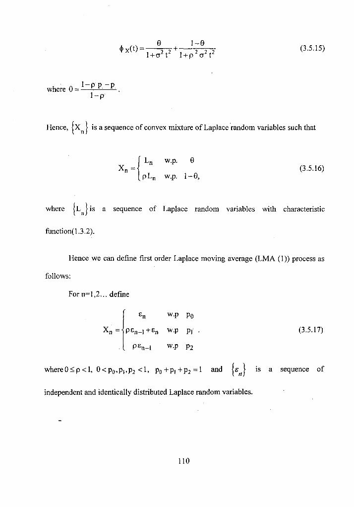
where 8 = 1-P'P, -P, 1 -p,

Hence, (xn] is a sequence of convex mixture of ~a~lacerandorn variables such that

where is a sequence of Laplace random variables with characteristic

function(l.3.2).

Hence we can define first order Laplace moving average (LMA (1)) process as

follows:

For n= 1,2.. . define

independent and identically distributed Laplace random variables.

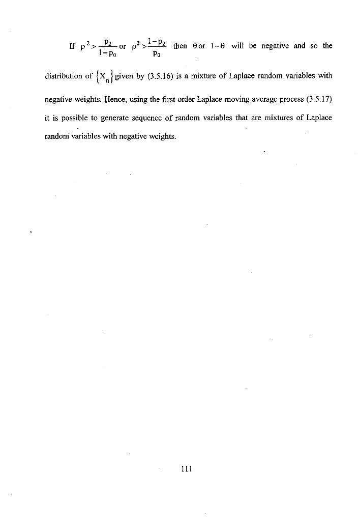
then 8 or 1 - 8 will be negative and so the P2 or p >- If p >- ~ - P O PO

distribution of X given by (3.5.16) is a mixture of Laplace random variables with { n l

negative weights. Hence, using the first order Laplace moving average process (3.5.17)

it is possible to generate sequence of random variables that are mixtures of Laplace

random' variables with negative weights.