A Neurodynamic Account of Spontaneous Behaviour Neurodynamic Account of Spontaneous Behaviour Jun Namikawa, Ryunosuke Nishimoto, Jun Tani* Brain Science Institute, RIKEN, Wako, Japan

A Neurodynamic Account of Spontaneous BehaviourJun Namikawa, Ryunosuke Nishimoto, Jun Tani*

Brain Science Institute, RIKEN, Wako, Japan

Abstract

The current article suggests that deterministic chaos self-organized in cortical dynamics could be responsible for thegeneration of spontaneous action sequences. Recently, various psychological observations have suggested that humansand primates can learn to extract statistical structures hidden in perceptual sequences experienced during activeenvironmental interactions. Although it has been suggested that such statistical structures involve chunking orcompositional primitives, their neuronal implementations in brains have not yet been clarified. Therefore, to reconstruct thephenomena, synthetic neuro-robotics experiments were conducted by using a neural network model, which ischaracterized by a generative model with intentional states and its multiple timescales dynamics. The experimentalresults showed that the robot successfully learned to imitate tutored behavioral sequence patterns by extracting theunderlying transition probability among primitive actions. An analysis revealed that a set of primitive action patterns wasembedded in the fast dynamics part, and the chaotic dynamics of spontaneously sequencing these action primitive patternswas structured in the slow dynamics part, provided that the timescale was adequately set for each part. It was also shownthat self-organization of this type of functional hierarchy ensured robust action generation by the robot in its interactionswith a noisy environment. This article discusses the correspondence of the synthetic experiments with the known hierarchyof the prefrontal cortex, the supplementary motor area, and the primary motor cortex for action generation. We speculatethat deterministic dynamical structures organized in the prefrontal cortex could be essential because they can account forthe generation of both intentional behaviors of fixed action sequences and spontaneous behaviors of pseudo-stochasticaction sequences by the same mechanism.

Citation: Namikawa J, Nishimoto R, Tani J (2011) A Neurodynamic Account of Spontaneous Behaviour. PLoS Comput Biol 7(10): e1002221. doi:10.1371/journal.pcbi.1002221

Editor: Olaf Sporns, Indiana University, United States of America

Received April 1, 2011; Accepted August 19, 2011; Published October 20, 2011

Copyright: � 2011 Namikawa et al. This is an open-access article distributed under the terms of the Creative Commons Attribution License, which permitsunrestricted use, distribution, and reproduction in any medium, provided the original author and source are credited.

Funding: The authors would like to thank Sony Corporation for providing the humanoid robot as a research platform. The present study was supported in partby a Grant-in-Aid for Scientific Research on Innovative Areas ‘‘The study on the neural dynamics for understanding communication in terms of complex heterosystems’’ from the Japanese Ministry of Education, Culture, Sports, Science and Technology. The funders had no role in study design, data collection and analysis,decision to publish, or preparation of the manuscript.

Competing Interests: The authors have declared that no competing interests exist.

* E-mail: [email protected]

Introduction

Our everyday actions are full of spontaneity. For example,

imagine that a man makes a cup of instant coffee every morning.

After he pours hot water into his mug, which is already filled with

a spoonful of coffee crystals, he may either add sugar first and next

add milk, or add milk first and then add sugar. Or, sometimes he

may even forget about adding sugar and notice it later when he

first tastes the cup of coffee. Some parts of these action sequences

are definite, but other parts are varied because we see spontaneity

in the action generation. Similar actions can be seen in

improvisations in playing jazz or in contemporary dance, where

musical phrases or body movement patterns are inspired freely

from one to another in an unpredicted manner. An essential

question is from where the spontaneity for generating voluntary

actions or images originates. The current article presents a model

prediction for the underlying neural mechanism.

We speculate that the necessary neural structures for generating

such spontaneous actions are acquired as the results of learning

from everyday experiences and practices while interacting with the

world. Gibson and Pick [1] once wrote that infants are active

learners who perceptually engage their environments and extract

information from them. In their ecological approach, learning an

action is not just about learning a motor command sequence.

Rather, it involves learning the possible perceptual structures

extracted during intentional interactions with the environment.

Other researchers [2–4] have proposed that perceptual structures

experienced during environmental interactions can be acquired by

using forward models that are assumed to be located in the

cerebellum. A forward model outputs the prediction of the next

sensation by receiving the inputs of the current sensation and

motor commands. Although this idea is generic and theoretical in

the sense that a forward model can predict the sensory outcomes of

arbitrary motor commands at every time step, it is impossible in

practice due to the combinatorial explosion problem if the motor

dimension becomes large. This problem is analogous to the frame

problem [5] that discusses that there are no rational means to stop

inferences about the outcomes of infinite action possibilities.

In humans, learning by environmental interaction does not

proceed with all possible combinations in motor command

sequences, but with more purposeful or intentional stances [1].

Therefore, it could be sufficient for humans to predict sensory

outcomes according only to purposeful behavior trajectories. With

regard to this theory, Tani [6] proposed an alternative idea that an

agent should learn mapping from a set of particular intentional

states with the consequent sensory sequences that are expected to

be experienced in corresponding purposeful environmental

interactions. Ay et al. [7] also proposed a prediction based model

PLoS Computational Biology | www.ploscompbiol.org 1 October 2011 | Volume 7 | Issue 10 | e1002221

to control an autonomous robot, but the model lacked internal

states. In the connectionist implementation by Tani and his

colleagues [6,8,9], the proposed neuro-dynamic model is operated

in three modes: generation, recognition and learning. In the

generation mode, the corresponding visuo-proprioceptive se-

quence is predicted for a given intentional state. The scheme

can generate mental simulation for future behaviors or motor

imagery (in terms of visuo-proprioceptive sequences) [10], and can

also generate the corresponding physical movement by sending the

next predicted proprioceptive state to the motor controller as the

next target. In the recognition mode, a given visuo-proprioceptive

sequence can be recognized by identifying the corresponding

intentional state through an iterative search to minimize the

prediction error. In the learning mode, the learning is formulated

as a process to search for the optimal values for both a common

synaptic weight matrix as well as a set of individual intentional

states that can regenerate all visuo-proprioceptive sequences of an

experience for training under minimum error criteria. This idea is

formally related to ‘‘active inference’’ [11], which can be regarded

as a form of predictive coding [12]. Friston [13] showed that the

three aspects of our neurodynamic model (generation, recognition

and learning) can be unified in terms of minimising prediction

error.

Moreover, it is presumed that the neural structures acquired

through intentional interactions with the environment should

support ‘‘compositionality’’ [14] or chunk knowledge for gener-

ating and recognizing the variety of complex actions [15–17].

Diverse intentional actions can be generated by combining a set of

reusable behavior primitives or chunks adaptively by following the

acquired rules. For example, an attempt at drinking a cup of water

can be decomposed into multiple behavior primitives, such as

reaching for a cup, grasping the cup and moving the cup toward

one’s mouth. Each behavior primitive can be re-used as a

component for other intentional actions, e.g., reaching for a cup to

take it away. Psychological observation on infant development as

well as adult learning have suggested that chunking structures in

perceptual streams can be extracted by statistical learning with

sufficient amounts of passive perceptual experiences [18,19] as

well as for active behavioral interactions [20]. Here, chunking

structures are represented by repeatable sensory sequences within

chunks and the probabilistic state transition among those chunks.

From his observation of skill acquisitions for food processing by

mountain gorillas, Byrne [21] proposed that actions can be

acquired with statistical structures through imitation. It is said that

juvenile gorillas take a few years to effectively imitate behaviors by

observing the mothers’ food processing behaviors, which are

characterized by nondeterministic transition sequences of behavior

primitives or chunks. After the skill acquisition by extracting the

underlying statistical structures, the primitive sequences of the

juveniles resemble those of their mothers. In another example,

improvisers of jazz music make substantial efforts into developing

vocabularies of musical patterns or phrases, which they then freely

combine and vary in a manner that is sensitive to the on-going

musical context [22]. In recent years, considerable evidence has

been assembled in support of statistical learning for both musical

pitch sequences [23] and rhythm [24] by organizing chunking

structures.

In searching for the neuronal mechanisms for chunking, a

monkey electrophysiological study [25] showed that some neurons

in the presupplementary motor area (preSMA) fire only at the

beginning of each chunk in the regeneration of trained sequences.

Also, a human behavior study [26] showed that inactivation of the

preSMA by transcranial magnetic stimulation (TMS) affects the

performance of regenerating sequences only when the TMS is

applied between the chunks after extensive learning of the

sequences with chunking structures. These studies suggest that

the preSMA might play a crucial role in segmenting sequences

into chunks. Sakai et al. [27] proposed a hierarchical function in a

cortical network, in which the prefrontal cortex and the preSMA

were responsible for the cognitive control of segmenting sequences

and selecting the next chunk, whereas more motor-related areas,

including the premotor cortex and the primary motor cortex, are

responsible for processing within each chunk. This proposal agrees

with the results of a monkey electrophysiological recording

[28,29], which showed that firing some cells in the preSMA and

the SMA encode specific sequences of joystick movement patterns

or specific transitions from one movement pattern to another.

Model studies by the authors have shown that chunking by

segmenting continuous sensory flow can be achieved by applying

the criteria of prediction error minimization to connectionist

models with local [17,30] and distributed [6,31] representation

schemes. Those model studies have also shown that a hierarchy is

indispensable in acquiring chunking structures. In the hierarchy,

the lower level learns to acquire a set of behavior primitives and

the higher level puts those primitives into sequences of intentional

actions. The idea of intentional actions is analogous to that by

Sakai et al. [32].

One essential question so far is how the next behavior primitives

or actions can be decided by following the learned statistical

expectation. For example, if we suppose that someone has learned

that the next behavior primitive to use is either primitive-A or

primitive-B, given an even chance from past experiences, it is

plausible to consider that either the primitives can be decided by

her/his conscious will or alternatively they can be determined

automatically without consciousness. Philosophers have discussed

for a long time whether humans have a ‘‘free will’’ to determine a

next action arbitrarily, and, if the free will exists, how it is

implemented in our minds [33–35]. Interestingly, recent neuro-

psychological studies on free decision [36,37] have suggested that

Author Summary

Various psychological observations have suggested thatthe spontaneously generated behaviors of humans reflectstatistical structures extracted via perceptual learning ofeveryday practices and experiences while interacting withthe world. Although those studies have further suggestedthat such acquired statistical structures use chunking,which generates a variety of complex actions recognizedin compositional manner, the underlying neural mecha-nism has not been clarified. The current neuro-roboticsstudy presents a model prediction for the mechanism andan evaluation of the model through physically groundedexperiments on action imitation learning. The modelfeatures learning of a mapping from intentional states toaction sequences based on multiple timescales dynamicscharacteristics. The experimental results suggest thatdeterministic chaos self-organized in the slower timescalepart of the network dynamics is responsible for generatingspontaneous transitions among primitive actions byreflecting the extracted statistical structures. The robust-ness of action generation in a noisy physical environmentis preserved. These results agree with other neuroscienceevidence of the hierarchical organization in the cortex forvoluntary actions. Finally, as presented in a discussion ofthe results, the deterministic cortical dynamics arepresumed crucial in generating not only more intentionalfixed action sequences but also less intentional spontane-ously transitive action sequences.

A Neurodynamic Account of Spontaneous Behaviour


the conscious will of initiating or selecting actions arbitrarily

follows certain neural activity that does not accompany awareness.

Libet et al. [36] showed that a conscious decision to press a button

was preceded for a few hundred milliseconds by a negative brain

potential, referred to as the readiness potential, which originates

from the SMA. In a functional magnetic resonance imaging

(fMRI) study, Soon et al. [37] demonstrated that brain activity is

initiated in the prefrontal cortex (PFC) and the parietal cortex up

to seven seconds before a conscious decision. It was further found

that the observed brain activity can predict the outcome of a

motor decision, which the subject did not consciously make, such

as pushing the left button by the left index finger or the right

button by the right index finger. This result implies the possibility

that even though someone can believe that he had consciously

decided a particular action among multiple choices, such as

primitive-A and primitive-B, the conscious decision was not the

direct cause of the action selection, but was the preceded neural

activity without awareness. It is also plausible to assume a purely

mechanist model in which an itinerant trajectory of neural

dynamics [38–41], instead of a conscious will, determines the next

behavior primitive to be performed.

The current article introduces a neuro-robotics experiment that

examines how statistical structures hidden in skilled behaviors can

be extracted via imitation learning and how the behaviors can be

regenerated by following the statistical structures. The experiment

uses a dynamic neural network model based on two essential ideas

from our previous proposals. First, in the dynamic neural network

model, a mapping from the initial states of the internal neural

dynamics to the expected visuo-proprioceptive trajectories is self-

organized, and the initial states encode various intentional states

for the resultant behavioral trajectories [9]. Second, the model

network employs multiple timescale dynamics [31,42] that allow

self-organization of the functional hierarchy, which is analogous to

the known cortical hierarchical network consisting of the PFC, the

preSMA, and the M1 [43,44] for generating goal-directed actions.

It is demonstrated that itinerant behaviors with accompanying

spontaneous transitions among behavior primitives can be

generated by reflecting the observed statistical structure and by

assuring the robustness of the behavior primitives against possible

noise during physical interactions, when deterministic chaos is self-

organized at the higher level of the functional hierarchy (the slow

dynamics part of the network). Based on the results, the current

article discusses the importance of deterministic neural dynamics

in action generation because they account for both itinerant

behaviors with accompanying spontaneous transitions of behavior

primitives and intentional fixed behaviors (repeatedly executable)

by the same dynamic mechanism. The article also discusses how

the model prediction presented can be applied in future

neurophysiological studies.

Results

Model OverviewThe proposed hierarchical dynamic neural network can be

regarded as a generative model of visuo-proprioceptive inputs

[6,11,31,45]. (Precise mathematical descriptions are provided in

the Methods section.) The network was divided into three levels

based on the value of the time constant t. Time constant t for each

unit primarily determined the timescale of the activation dynamics

of the unit (see Figure 1). The higher level consisted of slow neural

Figure 1. Hierarchical neural network consisting of three levels characterized by time constants of the neural activation dynamics.The higher-level, middle-level, and lower-level networks consist of neural units in which the activations are characterized by large (ts§20), moderate(tm~20), and small (tf~2) time constants, respectively. The visuo-proprioceptive input SS(t),M(t)T for each time t reaches the middle- and lower-level networks, and the middle level relays the input to the higher level. The lower-level network contains a set of modular networks generatingmotor commands, which, in turn, are forwarded to the gate. The gate, which prevents undesired motor commands from being released, is controlledby the middle-level network. Since the supplementary motor area (SMA) has been reported to trigger the movement by suppressing the inhibitorysignal exerted on the primary motor cortex [61], the middle-level and lower-level networks may correspond to the SMA and the primary motorcortex, respectively. The higher-level network may correspond to the prefrontal cortex (PFC), which projects to the SMA [62].doi:10.1371/journal.pcbi.1002221.g001



units with a larger time constant (ts§20), the middle level with a

moderate time constant (tm~20), and the lower level with a small

time constant (tf~2). The lower level was assembled with a set of

gated modular networks [46] that interacted directly with the

visuo-proprioceptive sequences. The higher level was mutually

connected to the middle level but was not directly connected to the

lower level. The middle level interacted with the lower level by

sending the gate opening signals and receiving the sensory inputs.

The parameters of this model were optimized to minimize

sensory prediction errors (i.e., maximizing the probability of the

predictions given the sensory data). In this sense, our model was

concerned with, and only with, perception. Action per se, was a

result of movements that conformed to the proprioceptive

predictions of the joint angles. This means that perception and

action were both trying to minimize prediction errors throughout

the hierarchy, where movement minimized the prediction errors at

the level of proprioceptive sensations. With this perspective, the

high-level network provided predictions of the middle-level

network that, in turn, provided predictions about which expert

will be engaged for prediction at the lowest (sensory) level. This

engagement depended upon the gating variables, which selected

the most appropriate expert in the lowest level of the hierarchy.

The network was trained to predict a set of given visuo-

proprioceptive sequences by optimizing the following two types of

parameters in order to minimize the prediction error: the synaptic

weights and the initial state of the internal units in the whole

network for each sequence [9]. This intuitively means that the

learning involves determining the dynamic function of the network

by changing the synaptic weights and also by inferring the

intention or goal of each action sequence. The learning scheme

was implemented by using the error back-propagation through

time algorithm [47]. Although the biological plausibility of error

back-propagation in neuronal circuits is a matter of debate, some

supportive evidence [48,49] and related discussions [50] exist. We

speculate that the retrograde axonal signal [50] conveying the

error information might propagate from the sensory periphery

area to the higher-order cortical area by passing through multiple

stages of synapses and neurons for modulating the intentional

states.

After minimizing the error, each visuo-proprioceptive sequence

of the training can be regenerated by setting the initial state of the

internal units with the optimized value. Because the initial state

specified the expected visuo-proprioceptive sequence, the initial

states are considered to represent the intentions of generating

specific actions. The forward dynamics of the trained network can

generate motor imagery in terms of visuo-proprioceptive sequenc-

es by feeding back the sensory prediction computed at the previous

time step into the current sensory inputs without the accompa-

nying physical movements (closed-loop operation). However, the

physical movements can be generated by sending the next time

step prediction of the proprioceptive states (joint angles) to the

motor controller as the target (open-loop operation).

As one aspect of our work, we examine how the dynamic

function of each level can be differentiated depending on the

timescale differences. To study the timescale characteristics in

more detail, we investigated cases applying various values of the

time constant ts set in the higher-level network.

Design of Robot ExperimentsExperiments on imitation learning of actions were conducted on

a small humanoid robot platform (Sony Corporation), and the

movie of a demonstration is available (http://www.bdc.brain.

riken.jp/tani/mov/PLoS11.html). The robot experiments on the

aforementioned dynamic neural network model involved imitative

training of the sequences of primitive actions and autonomous

generation of those imitated behaviors. The target primitive action

sequences to be imitated were designed with a statistical structure

and with transitioning of the primitive actions, and the sequences

were directly tutored to the robot, i.e., a human assistant directly

guided the movements of both hands of the robot by grasping

them. In the beginning of each training sequence, the assistant

guided both hands of the robot, which was positioned in front of a

workbench (see Figure 2). A cubic object was placed on the

workbench at one of three positions (center, 6 cm left of center,

and 6 cm right of center), and the assistance repeated primitive

actions of grasping the object, moving it to one of the three

positions and releasing it by guiding the hands of the robot while

deciding the next object position randomly with equal probability

(~50%). Although the hands of the robot were guided by the

assistant, the visuo-proprioceptive sequences were recorded for

later training. The neural network was trained in an off-line

manner, since all training sequences gathered at each teaching

session were used for the subsequent consolidation learning. Thus,

the neural network learned to predict visuo-proprioceptive

sequences on the basis of the experiences obtained during the

imitative training session. Note that no explicit cues for segmenting

the sequences into primitive actions were prepared. The related

chunking structures were acquired via iterative experiences of the

continuous visuo-proprioceptive sequences.

After the imitative training, each training sequence was

regenerated by setting the initial state with the optimized value.

For the subsequent analysis, primitive action sequences were

generated and recorded for far longer than the training sequences.

For the detailed analysis on the possible dynamic structures

Figure 2. Schematic diagram of the teaching sequence generation process. As shown on the left, the assistant selected one actionrandomly while guiding the hands of the robot to move the cubic object. For each action, the assistant started from a posture in which the hands ofthe robot were open and then the assistant grasped the object by using the hands of the robot. Whenever the object was moved to another position,the assistant released the object and returned the robot hands to the starting posture for a brief period of time. The graph on the right depicts thetrajectory of the center of the object captured by the vision sensor.doi:10.1371/journal.pcbi.1002221.g002



acquired in the network model, the itinerant trajectories by motor

imagery for longer steps were also generated.

Training and Action GenerationThe network was trained by a learning scheme in which the

higher-level time constant ts was 20, 50, and 100 [45] (see the

Methods section for details). For each condition of the higher-level

time constant, training trials were conducted for 100 sample

networks with different initial parameters and training data.

Descriptions of the learning parameters are provided in the

Methods section. The trained networks were tested for pseudo-

generation by motor imagery, and it was shown that the networks

regenerated primitive action sequences pseudo-stochastically in

their deterministic itinerant trajectories. Here, pseudo-stochasticity

denotes stochasticity observed through the discretization of

deterministic continuous value sensory sequences into symbolically

labeled primitive action sequences. The action generation test by

motor imagery, also described in the Methods section, revealed

that the trained neural networks were able to create novel

sequential combinations of the primitive actions that were not

contained in all teaching sequences. This implies that primitive

actions can be generated pseudo-stochastically, as taught in all ts

conditions.

We also tested cases of training primitive action sequences

having different probabilities of selected primitive actions in a

specific object position, as detailed in Text S1. It was observed that

these probabilities were reconstructed in the generation of the

primitive action sequences by motor imagery. The results suggest

that the network is capable of extracting underlying statistical

structures in the imitated primitive action sequences.

Next, we tested the generation of actual actions of interacting

with the physical environment by the robot. First, the behavior of

the robot was generated from each acquired initial state with the

higher-level time constant, ts set at 100. Although it was observed

that the trained primitive action sequences can be regenerated

exactly during the initial period (7.3 primitive action transitions on

average), the sequences gradually became different from the

trained ones. It was considered that this result was due to the initial

sensitivity characteristics organized in the trained network.

Then, we tested actual action generations for cases of different

values of time constant ts. Although no particular difference was

found between the cases with a different ts in the action generation

test by the motor imagery mode, the stability in actual action

generation in the physical environment was different for each ts.

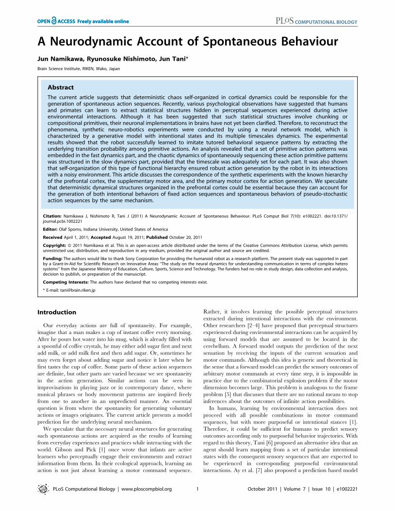
The success rate for moving the object without dropping it was

evaluated for each trained network with a different time constant

ts. Figure 3 shows the frequencies of the networks classified

according to the success rate, where populations of 40 individual

networks were trained for each time constant ts. In all cases we

found a network with a 100% success rate, but the average success

rate was different for each ts. The success rate for ts~100 was

higher than the success rates for the other values of ts.

This result indicates that motor patterns can be generated stably

in the physical environment when ts is set larger than tm.

Self-Organized Functional HierarchyAs mentioned in the previous section, the stability in actual

action generation is dependent on the timescale characteristics.

This fact implies that the developed dynamic structure is different

for each timescale condition. In the following we discuss the

characteristics of the self-organized functional hierarchy in terms

of the timescale differences. As an example, Figure 4 illustrates the

sensory motor sequences and neural states. It can be seen that an

action primitive of moving the object to the left, to the right, or to

the center consisted of a few different gate openings, which

generated sequential switching of the stored reusable motor

patterns, such as reaching for the object, picking up the object, and

moving back its hand position to the starting posture. It is

Figure 3. Success rate r of a robot controlled by a neural network to move an object. For example, r~3=4 indicates 75% success ofmoving the object without dropping it. The graph depicts the frequencies of networks occurring in certain ranges of the success rate. We recordedthe behaviors of the robot for up to 30 trials of moving the object for 40 sample networks. The average success rates for the higher-level timeconstant ts of 20, 50, and 100 were 51%, 75%, and 78%, respectively.doi:10.1371/journal.pcbi.1002221.g003



considered that the middle- and higher-level network dynamics

encoded the combinations of these reusable motor patterns into

primitive actions and further into their stochastically switching

sequences.

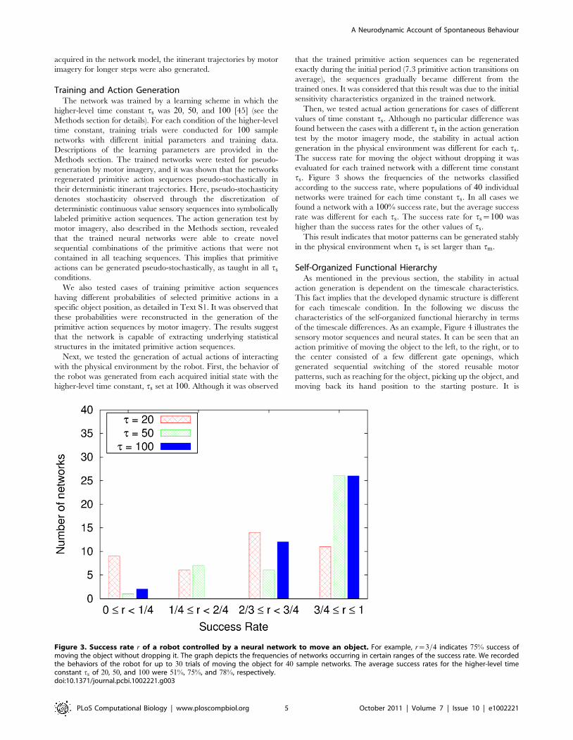
The auto-correlation for each ts is shown in Figure 5 to clarify

the timescale characteristics. The auto-correlation measures the

correlation between values at different points in time and is

sometimes used to find repeating patterns. A high auto-correlation

at time difference t means that similar values appear repeatedly

with a period of t. We found a periodic pattern of auto-correlation

common to both the visuo-proprioception and the middle-level

network units in the ts cases. This periodicity is considered to

occur because the periodicities of all primitive actions were

approximately the same. Conversely, such a periodic pattern was

not found in the higher-level network if the higher-level network

had a relatively large time constant. The characteristics of auto-

correlation seem to correspond to the functionality obtained by

each subnetwork.

To examine the functionality developed at each subnetwork,

we investigated the effect of artificial lesions in the higher-level

network. To model the artificial lesions, we removed all the

neurons in the higher-level network. Figure 6 is a comparison of

the trajectory of the object position captured by the vision sensor

in the motor imagery mode for the normal case and that with the

artificial lesions. In this figure, we used networks having a 100%success rate in actual action generation. If the trajectory

generated by the network traced the test data (see Figure 2),

the network moved the object by correctly using the hands. When

the time constant of the higher level was set as 100, the network

was able to generate each single primitive action correctly, even if

the higher level was removed. However, in this case, the

capability for combining diverse primitive actions significantly

deteriorated. For ts set at 50 or 20, the removal of the higher

level significantly affected the generation of each primitive action.

This implies that the functions for generating each primitive

action and for generating stochastic combinations of these actions

were self-organized and became segregated between the higher

and the middle/low levels if ts was set significantly larger than tm

and tf . Otherwise, both functions were self-organized but not

segregated. That is, the functions were distributed throughout the

entire network. In this situation, a lesion in the higher-level

network could affect the lower sensory-motor control level. The

abovementioned functional segregation between levels could

contribute to the stability in the action performance evaluated

in Figure 3.

In addition, the maximum Lyapunov exponents for the

subnetworks were computed while varying ts as 20, 50, and

100 (see Methods for details). Here, tm and tf were fixed at 20and 2, respectively. The computation was repeated for 100 neural

networks trained using different initial synaptic weights but under

the same learning condition. If the Lyapunov exponent is found

to be positive for specific subnetworks or for the entire network,

then the intrinsic dynamics of the subnetworks or network are

identified as chaotic. In chaotic dynamics, almost any minute

change in an internal neural state brings about a drastic change

in subsequent network outputs because of the dependence on the

initial conditions. Therefore, it can be inferred that subnetworks

having positive maximum Lyapunov exponents act to combine

action primitives with pseudo-stochasticity. The results are

summarized in Table 1. The maximum Lyapunov exponent of

the entire network was positive for all values of ts. This was

expected because the network was able to generate pseudo-

stochastic primitive action sequences regardless of the value of ts.

However, the values of the maximum Lyapunov exponent were

negative in the higher level and the middle level, when the

higher-level network had a small time constant ts~20. These

results indicate that the function to generate chaos was globally

distributed over the entire network. In contrast, when the higher-

level network was set with a large time constant, i.e., ts~100, the

maximum Lyapunov exponent of the higher-level network

became positive in most cases (94 out of 100 network learning

cases), whereas that of the middle-level network became negative.

Figure 4. Time series generated by a trained network (ts~~20, 50, and 100). In the vision case, the two lines correspond to the relativeposition of the object (red: horizontal, green: vertical). Each label over the vision sensor values denotes the object position (L: left, C: center, and R:right). In proprioception, 2 out of a total of 8 dimensions were plotted (red: left arm pronation, green: left shoulder flexion). The lower three figuresshow the time series described by grayscale plots, where the vertical axis represents the indices of the neural units. A long sideways rectangle thusindicates the activity of a single unit over many time steps.doi:10.1371/journal.pcbi.1002221.g004



The abovementioned results demonstrate that if the time

constant of the higher level is sufficiently larger than the time

constants of the other regions, then chaotic dynamics are formed

primarily in the higher-level network, separate from the other

regions. These results agree with the results in the case having

lesions. Furthermore, the abovementioned analysis on the

artificial lesion cases indicates that the segregation of chaos

from the middle and lower levels provides more stable motor

generation. In summary, if we regard our neurodynamic model

as a generative model of visuo-proprioceptive sequences, the

anatomical segregation between sequential dynamics and motor

primitives (e.g., within premotor and motor cortex, respectively)

emerges only when we accommodate the separation of temporal

scales implicit in the hierarchical composition of those

sequences.

Finally, we examined how the generation of chaos that allows

pseudo-stochastic transition among action primitives depends on

the characteristics of the training sets. For this purpose, the

networks with ts set at 100 were trained by changing the length

(i.e., number of transitions of primitive actions) of the training

sequences, as detailed in Text S1. It was observed that the

possibility of generating chaos is reduced as the length of the

training sequences is reduced. If no chaos was generated, it was

observed that neural activity in the higher-level network often

converged to a fixed point some steps after the tutored sequences

were regenerated. This result implies that the mechanism for

spontaneous transition by chaos can be acquired only through

training of long sequences that contain statistically enough

probabilistic transitions for generalization.

Discussion

Spontaneous Action Generation by ChaosThe current experimental results revealed that the chaos self-

organized in the higher-level network with slow-timescale

dynamics facilitates spontaneous transitions among primitive

actions by following statistical structures extracted from the set

of visuo-proprioceptive sequences imitated, whereas primitive

actions were generated in the faster-timescale networks in the

lower level. The finding was repeatable in the robotic experiments,

provided that the timescale differences were set adequately among

the different levels of subnetworks. The results appear to be

consistent with human fMRI recordings, which indicate that free-

decision-related activity without consciousness is slowly built up in

the PFC seconds before the conscious decision [37]. This buildup

of activity in the PFC could initiate a sharp response in the SMA

just a few hundred milliseconds before the decision [36].

Activation in the SMA leads to immediate motor activity [28],

and buildup of action-related cell activity in the PFC in the

monkey brain takes a few seconds, whereas that in the primary

motor area takes only a fraction of a second [51]. These

observations support recent arguments concerning the possible

hierarchy along the rostro-caudal axis of the frontal lobe. Badre

and D’Esposito [43] proposed that levels of abstraction might

decrease gradually from the prefrontal cortex (PFC) through the

premotor cortex (PMC) to the primary motor cortex (M1) along

the rostro-caudal axis in the frontal cortex in both the monkey

brain and the human brain [44]. Here, the rostral part is

considered to be more integral in processing information than the

Figure 5. Auto-correlation for each neural unit, shown by grayscale plots. The vertical axes denote the indices of the neural units, and thehorizontal axes denote the length of time.doi:10.1371/journal.pcbi.1002221.g005



caudal part in terms of its slower timescale dynamics. By

considering the possible roles of the M1, such as encoding the

posture or direction of limbs [52,53], it is speculated that this

hierarchy in the frontal cortex contributes to the predictive coding

of proprioceptive sequences through the M1 in one direction, and

to that of visual sequences in the other direction via the possible

connection between the inferior parietal cortex and the SMA,

known as the parieto-frontal circuits [54,55].

Additionally, our experiments showed that the behavior

generation of the robot in the real environment becomes

substantially unstable when the timescale of the higher-level

network is set smaller, that is, when the timescale is similar to the

values in the middle-level network. Our analysis in such cases

revealed that the two functions of generating primitive motor

patterns and sequencing them cannot be segregated in the whole

network if the chaos dynamics tend to be distributed. Gros [56],

Figure 6. Trajectory of the object position captured by the vision sensor in the motor imagery mode. Left: normal case, Right: removalof the higher-level network case (lesion case).doi:10.1371/journal.pcbi.1002221.g006

Table 1. Maximum Lyapunov exponents of various regions (mean of 100 sample networks).

Time constant ts of the higher level Entire network Middle-level network Higher-level network

20 0:005482 (82%) {0:004990 (32%) {0:005069 (5%)

50 0:003746 (97%) {0:006564 (0%) {0:000068 (57%)

100 0:002471 (99%) {0:007424 (0%) 0:000533 (94%)

The percentages in parentheses represent the probability that the maximum Lyapunov exponent of each network was positive in multiple training trials.doi:10.1371/journal.pcbi.1002221.t001



who referred to higher-level as the reservoir and to the middle/low

levels as attractor networks, also discussed the generation and

stabilization of transient state dynamics, in terms of attractor ruins.

The discussion supports one’s opinion that the slower timescale

part exhibits robustness of influence of external stimuli. Therefore,

it is concluded that the hierarchical timescale differences, which

are assumed to be in the human frontal cortex and to be

responsible for the generation of voluntary actions, are essential for

achieving the two functions of freely combining actions in a

compositional manner and generating them stably in a physical

environment.

Deterministic versus Stochastic ProcessThe uniqueness in the presented model is that deterministic

chaos is self-organized in the process of imitating stochastic

sequences, provided that sufficient training sequences are utilized

to support the generalization in learning (it was observed that the

reduction of length in the training sequences can hinder the self-

organization of chaos). Therefore, it might be asked why

deterministic dynamical system models are considered more

crucial than stochastic process models such as the Markov Chain

[57] or Langevin equation [58,59]. A fundamental reason for

focussing on deterministic (as opposed to stochastic) dynamics is

that they allow for mean field approximations to neuronal

dynamics and motor kinetics. This is important because although

individual neuronal dynamics may be stochastic, Fokker Planck

formulations and related mean field treatments render the

dynamics deterministic again; and these deterministic treatments

predominate in the theoretical and modelling literature. Further-

more, we speculate that deterministic neuronal dynamic systems

are indispensable for generating both spontaneous behaviors and

intentional behaviors under the same dynamic mechanism,

especially by applying the initial sensitivity characteristics. When

the system is initiated from unspecified initial states of the internal

units, the resultant itinerant behavioral trajectories exhibit

spontaneous transitions of primitive actions by reflecting the

statistical structures extracted through the generalization in

learning. However, it is also true that a particular sequence of

shorter length can be regenerated by resetting with the

corresponding initial state values by the deterministic nature of

the model. Our robotics experiments showed that the robot can

regenerate trained sequences up to several transitions of primitive

actions under a noisy physical environment. In addition, our

preliminary experiments suggested that longer primitive action

sequences can be stably regenerated if those intentional sequences

are trained more frequently than other non-intentional ones. This

implies that frequently activated fixed sequences can be remem-

bered by cash memories of their initial states. If the Markov chain

model is employed for reconstructing the same feature, the model

must handle the dualistic representation, namely the probabilistic

state transition graph for generating itinerant behaviors and the

deterministic linear sequence for generating each intentional

behavior.

Empirical support for the idea of encoding action sequences by

initial states can been found. Tanji and Shima [28] found that

some cells in the SMA and the preSMA fire during the

preparatory period immediately before generating specific prim-

itive action sequences in the electrophysiological recording of

monkeys. The results can be interpreted such that those cell firings

during the preparatory period may represent the initial states that

determine which primitive action sequences to be generated

subsequently. In the future, if this study can be extended to

simultaneous observations of the populations of animal cells during

spontaneous action sequence generation by employing the recent

developments of multiple-electrode recording techniques, our

model prediction can be further evaluated.

Methods

Model ImplementationThe evolution of a continuous-time-rate coding model is defined

as

t _uu~{uzWf (u)zI , ð1Þ

where t is a time constant, W is a weight matrix, I is a bias vector,

and f is the activation function of a unit (typically the sigmoid

function or tanh). When this differential equation is put into the

form of an approximate difference equation with step size d, we

obtain

un~(1{d

t)un{1z

d

t(Wf (un{1)zI): ð2Þ

In the present paper, we assume d~1 without the loss of

generality.

As the hierarchical neural network for controlling a humanoid

robot, we used a mixture of the recurrent neural network (RNN)

experts model [45], in which the gating network is a multiple-

timescale RNN [31]. The mixture of RNN experts consists of

expert networks together with the gating network. All experts

receive the same input and have the same number of output units.

The gating network receives the previous gate opening values and

the input, and then controls the gate opening. The role of each

expert is to compute a specific input-output function, and the role

of the gating network is to decide which single expert is the winner

on each occasion. In the present paper, the set of expert RNNs is

referred to as the lower-level network. The middle- and higher-

level networks differentiated by time constants are contained in the

gating network.

The dynamic states of the lowest-level neural networks (the

mixture of experts) at time n are updated according to

u(i)n ~(1{

1

tf)u(i)

n{1z1

tf(WiSf (u(i)

n{1),xn{jTzI i), ð3Þ

y(i)n ~f (Vif (u(i)

n )zJ i), ð4Þ

yn~XN

i~1

g(i)n y(i)

n , ð5Þ

where xn is an input vector representing the current visuo-

proprioception, and yn is an output vector representing the

predicted visuo-proprioception. Here, f denotes a component-wise

application of tanh, N is the number of experts, and j is the

feedback time delay of the controlled robot (in the experiment

j~3). In the present paper, Sa,bT denotes the concatenation of

vectors a and b. For each i, the terms g(i)n , u(i)

n , and y(i)n denote the

gate opening value, the internal neural state, and the output state

of the expert network i, respectively. The gate opening vector gn

represents the winner-take-all competition among experts to

determine the output yn. The gate opening vector gn is the output

of the gating network, defined by



umn ~(1{

1

tm)um

n{1z1

tm(WmSf (um

n{1,usn{1),xn{j,gn{jTzIm), ð6Þ

usn~(1{

1

ts

)usn{1z

1

ts

(Wsf (usn{1,um

n{1)zI s), ð7Þ

bn~Vmf (umn )zJm, ð8Þ

g(i)n ~

exp(b(i)n )

XN

k~1exp(b(k)

n ), ð9Þ

where umn and us

n denote the internal neural states of the middle-

level and higher-level networks, respectively. To satisfy g(i)n §0 andPN

i~1 g(i)n ~1, Equation (9) is given by the soft-max function. Using

the sigmoid function denoted by sigmoid(x)~1

1zexp({x),

Equation (9) can be expressed as

g(i)n ~sigmoid(b(i)

n {lnX

k=i

exp(b(k)n )): ð10Þ

This equation indicates that the output of the gating network is

given by the sigmoid function with global suppression. Note that

the visuo-proprioceptive input xn{j enters the state Equations (3)

and (6). During imagery, this is replaced by its prediction yn{j so

that these equations become (in discrete form) nonlinear

autoregression equations that embody the learned dynamics.

During inference and action, optimising the parameters of these

equations can be thought of as making them into generalised

Bayesian filters such that the predictions become maximum a

posterior predictions under the (formal) priors on the dynamics

specified by the form of these equations.

Learning MethodThe procedure for training the hierarchical neural network

model is organized into the following two phases:

1. We first train the experts (lower level) by optimizing their

parameters. Crucially, in this phase, the gating variables are

treated as unknown parameters and are optimized according to

the teaching sensory data.

2. We then train the gating networks (middle and higher levels) by

optimizing their parameters to predict the gating variables

optimized in Phase (1).

The training procedure progresses to phase (2) after the

convergence of phase (1). For each phase, the learning involves

choosing the best parameter based on the maximum a posteriori

estimation. A learning algorithm with a likelihood function and a

prior distribution was proposed in [45]. In the following, we

describe a learning algorithm corresponding to the above

description of the hierarchical neural network model.

Probability distribution. To define the learning method, we

assign a probability distribution to the hierarchical neural network.

Here, the adjustable parameters of an expert network i and a gating

network are denoted as qi~(Wi,Vi,I i,J i,u(i)0 ) and qg~(Wm,Ws,

Vm,Im,I s,Jm,um0 ,us

0), respectively. The estimate ggn of the gate

opening vector is given in terms of the variable bbn, as follows:

gg(i)n ~

exp(bb(i)n )

XN

k~1exp(bb(k)

n ): ð11Þ

Let X~(xn)Tn~1 be an input sequence of visuo-proprioception,

and let bbn and ª be parameters, where ª is a set of parameters

given by ci~(qi,si). Given X , bbn, and ª, the probability density

function (p.d.f.) for the output yn is defined by

p(ynjX ,bbn,ª)~XN

i~1

gg(i)n p(ynjX ,ci), ð12Þ

where p(ynjX ,ci) is given by

p(ynjX ,ci)~(1ffiffiffiffiffiffi

2pp

si

)d exp({jjy(i)

n {ynjj2

2s2i

), ð13Þ

where d is the output dimension, and y(i)n is the output from expert

i, as computed by Equations (3), (4), and (5) with the parameter qi.

Thus, the output of the model is governed by a mixture of normal

distributions. These equations result from the assumption that the

observable sequence data is embedded in additive Gaussian noise.

Minimizing the mean square error is equivalent to maximizing the

likelihood determined by a normal distribution for learning in a

single neural network. Therefore, Equation (13) is a natural

extension of neural network learning.

Given a parameter set h~((bbn)Tn~1,ª) and an input sequence X ,

the probability of an output sequence Y~(yn)Tn~1 is given by

p(Y jX ,h)~PT

n~1p(ynjX ,bbn,ª): ð14Þ

The function L of data set D~(X ,Y ) parameterized by h is

defined by the product of the likelihood p(Y jX ,h) and a prior

distribution, denoted as

L(D,h)~ln½p(Y jX ,h)Q(h)�, ð15Þ

where Q(h) is the p.d.f. of a prior distribution given by

Q(h)~ PT{1

n~1PN

i~1

1ffiffiffiffiffiffi2pp

zexp({

(bb(i)nz1{bb(i)

n )2

2z2): ð16Þ

This equation indicates that the vector bbn is governed by N-

dimensional Brownian motion. The prior distribution has the

effect of suppressing changes of the gate opening values. We can

now optimize the unknown parameters in Equation (15) with

respect to function L. These parameters include the variables

underlying the optimum gating, the connection strengths of the

lower level, and the parameters controlling the variance of sensory

noise. We next consider Phase 2, in which the parameters of the

gating network are optimized.

Assume that Dg~(X ,(ggn)Tn~1) is given. We define the likelihood

L(Dg,hg) by the multinomial distribution

p(ggnjgn)~1

Z(ggn)PN

i~1(g(i)

n )gg(i)n , ð17Þ



L(Dg,hg)~XT

n~1

ln p(ggnjgn), ð18Þ

where Z(ggn) is the normalization constant, and gn is given by X

and hg. Note that gn in Equation (18) is calculated by the teacher

forcing technique [60], i.e., using ggn{j instead of gn{j in Equation

(6). In addition, because of the term xn{j on the right-hand side of

Equation (6), gn cannot be computed if nƒj. Then, we assume

that gn~ggn if nƒj. If we consider g(i)n to be the probability of

choosing an expert i at time n, maximizing L(Dg,hg) is equivalent

to minimizing the Kullback-Leibler divergence

DKL((ggn)Tn~1jj(gn)T

n~1)~XT

n~1

XN

i~1

gg(i)n ln (

gg(i)n

g(i)n

): ð19Þ

Maximum a posteriori estimation. The learning method

chooses the best parameters h and hg by maximizing (or

integrating over) the likelihood L(D,h) and L(Dg,hg). More

precisely, we use the gradient descent method with a momentum

term as the training procedure. The model parameters at learning

step t are updated according to

h�(tz1)~h�(t)zaDh�(t), ð20Þ

Dh�(t)~LL(D�,h�(t))

Lh�(t)zgDh�(t{1), ð21Þ

where (D�,h�) is (D,h) or (Dg,hg). Here, a is the learning rate, and

g is the momentum term parameter.

Although we have explained only the case in which the training

data set D is a single sequence, the proposed method can easily be

extended to the learning of several sequences by using the sum of

the gradients for each sequence. When several sequences are used

as training data, initial states u(i)0 , um

0 , and us0 and an estimate ggn of

the gate opening vector must be provided for each sequence.

Acceleration of gating network learning. In principle, the

present training procedure is defined by Equations (21) and (20).

However, the learning for a gating network sometimes becomes

unstable, and so the likelihood L(Dg,hg) often decreases when

updating the parameter hg with certain learning rates [45]. Of

course, if we use sufficiently small learning rates, the likelihood

does not decrease for any learning step. However, considerable

computational time is required. Hence, to practically accelerate

gating network learning, we update the learning rate adaptively by

the following algorithm.

1. For each learning step, updated parameters are computed by

Equations (21) and (20) by applying the learning rate a, and the

rate r defined by

r~DKL((ggn)T

n~1jj(g0n)Tn~1)

DKL((ggn)Tn~1jj(gn)T

n~1)ð22Þ

is also computed, where (gn)Tn~1 and (g0n)T

n~1 are sequences of the

gate opening values corresponding to the current parameters and

the updated parameters, respectively.

2. If rwrth, then a is replaced with aadec, and return to (1).

Otherwise, go to (3).

3. If rv1, then a is replaced with aainc. Go to the next learning

step.

In the present study, we use rth~1:1, adec~0:7, and ainc~1:05.

Parameter Settings for TrainingIn the training processes, we used 24 training sequences,

including 20 action primitives of moving an object to the left, to

the center, and to the right. The time constants for the lower-level

and middle-level networks were set to tf~2 and tm~20,

respectively. The time constant for the higher level was chosen

to be ts§20. The number of experts was N~16, and the number

of internal units for each expert was 10. There were 30 internal

units for the middle-level network and 30 for the higher-level

network, i.e., the total number of internal units in the gating

network was 60. Each element of the matrices and biases of either

an expert or a gating network was initialized by random selection

from the uniform distribution on the interval ½{ 1

M,

1

M�, where

M is the number of internal units. The initial states for the experts

and the gating network were also initialized randomly from the

interval ½{1,1�. The parameters (bbn)Tn~1 and s were initialized

such that bbn~0 for each n and s~1, respectively. Since the

maximum value of L(D,h) depends on the total length T of the

training sequences and the dimension d of the output units, the

learning rate a was scaled by a parameter ~aa that satisfies a~1

Td~aa.

The parameter settings were ~aa~0:01, g~0:9, �ss~0:05, and z~1.

For each training trial, we conducted learning for the experts up

to 20,000 steps and learning for the gating network up to 30,000steps. We performed training of the experts for 100 samples having

different initial parameters and training data. In addition, for each

set of trained experts, we performed training of the gating network

while varying the higher-level time constant ts at 20, 50, and 100.

As a result, 100 samples of a mixture of RNN experts were

provided for each condition of the higher-level time constant.

Robotic PlatformThe behaviors of the robot were described by a 10-dimensional

time series, which consists of proprioception (an eight-dimensional

vector representing the angles of the arm joints) and vision sense (a

two-dimensional vector representing the object position). On the

basis of the visuo-proprioception, the neural network generated

predictions of the proprioception and vision sense for the next time

step. This prediction of the proprioception was sent to the robot in

the form of target joint angles, which acted as motor commands

for the robot to generate movements and interact with the physical

environment. This process, in which values for the motor torque

were computed from the desired state, was considered at a

computational level to correspond to the inverse model. This

inverse computation process was preprogrammed in the robot

control system. Changes in the environment, including changes in

the object position and changes in the actual positions of the joints,

were sent back to the system as sensory feedback.

Action Generation TestWe demonstrate how a trained network learns to generate

combinations of primitive actions. Let us consider a sequence of

symbols labeled according to the object position, e.g.,

‘‘CLRLRCL� � �’’, where C, L, and R are the center, left, and

right positions, respectively. Let x be a block if x is a finite

sequence of symbols. An n-block is simply a block of length n. To

evaluate the performance in creating novel sequential combina-

tions, we counted the number of n-blocks that appeared in the

visuo-proprioceptive time series generated by the network. We

computed the ratio of the number of n-blocks generated by the



network to the total number of possible n-blocks (note that the

total number of possible n-blocks is 3:2n{1). Figure 7 shows the

ratios averaged over 100 sample networks with higher-level time

constants ts of 20, 50, and 100 in the motor imagery mode. Note

that the teaching sequences do not include all acceptable

combinations, because the teaching data are finite.

Maximum Lyapunov ExponentThe maximum Lyapunov exponent of a dynamic system is a

quantity that characterizes the rate of exponential divergence from

the perturbed initial conditions. Consider two points, Z0 and

Z0zdZ0, in a state space, each of which generates an orbit in the

space by the dynamic system. The maximum Lyapunov exponent

l can be defined as

l~ limt??

1

tln

dZ(t)

jdZ0j, ð23Þ

where dZ0 is the initial separation vector of two trajectories, and

dZ(t) is the separation vector at time t.To evaluate the maximum Lyapunov exponent for each neural

network, we computed 100 sample sequences of 100,000 time

steps with a random initial state and an initial separation vector by

a numerical simulation. In the numerical simulation, a network

received predictions of the visuo-proprioception generated by the

network itself as input for the next step. When the maximum

Lyapunov exponent of a middle- or higher-level network was

measured, we computed the dynamics of the entire network, but

evaluated a separation vector containing only the component of a

subnetwork as a middle- or higher-level component. This method

measures the contribution of the subnetwork to the initial

sensitivity of the dynamics. Note that if the subnetwork has a

positive Lyapunov exponent, as measured in the abovementioned

manner, then the entire network also has a positive Lyapunov

exponent.

Supporting Information

Text S1 Supporting online material for ‘‘A Neurody-namic Account of Spontaneous Behaviour.’’ This file

describes two types of additional experiment, namely ‘‘Recon-

struction of probability’’ and ‘‘Dependency on training data

length’’. These experimental results clarify the possible relation

between chaos generated and the condition of the statistical

learning employed in the model network.

(PDF)

Author Contributions

Conceived and designed the experiments: JN RN JT. Performed the

experiments: RN. Analyzed the data: JN. Wrote the paper: JN JT.

Designed the software used in analysis: JN.

References

1. Gibson E, Pick A (2000) An ecological approach to perceptual learning and

development. Oxford University Press, USA.

2. Ito M (1970) Neurophysiological aspects of the cerebellar motor control system.

Int J Neurol 7: 162–176.

3. Uno Y, Kawato M, Suzuki R (1989) Formation and control of optimal trajectory

in human multi-joint arm movement. Biol Cybern 61: 89–101.

4. Wolpert D, Ghahramani Z, Jordan M (1995) An internal model for sensorimotor

integration. Science 269: 1880–1882.

5. McCarthy J (1963) Situations, actions, and causal laws. Technical Report AIM-

2, Artificial Intelligence Project, Stanford University.

6. Tani J (2003) Learning to generate articulated behavior through the bottom-up

and the top-down interaction processes. Neural Netw 16: 11–23.

Figure 7. Performance for creating novel sequential combinations of primitive actions. This graph shows the ratio of the number of n-blocks generated by the network to the total number of possible n-blocks. The total number of acceptable combinations (of length n of the primitiveaction series) was 3:2n{1 . To evaluate the ratio, the data for 100 sample networks were averaged for each condition of the higher-level time constantts in a numerical simulation.doi:10.1371/journal.pcbi.1002221.g007



7. Ay N, Bertschinger N, Der R, Guttler F, Olbrich E (2008) Predictive information

and explorative behavior of autonomous robots. Eur Phys J B 63: 329–339.8. Tani J, Ito M, Sugita Y (2004) Self-organization of distributedly represented

multiple behavior schemata in a mirror system: reviews of robot experiments

using rnnpb. Neural Netw 17: 1273–1289.9. Nishimoto R, Namikawa J, Tani J (2008) Learning multiple goal-directed actions

through self-organization of a dynamic neural network model: A humanoidrobot experiment. Adapt Behav 16: 166–181.

10. Jeannerod M (1994) The representing brain: Neural correlates of motor

intention and imagery. Behav Brain Sci 17: 187–202.11. Friston K, Mattout J, Kilner J (2011) Action understanding and active inference.

Biol Cybern. pp 1–24.12. Rao R, Ballard D (1999) Predictive coding in the visual cortex: a functional

interpretation of some extra-classical receptive-field effects. Nat Neurosci 2:79–87.

13. Friston K (2010) The free-energy principle: a unified brain theory? Nat Rev

Neurosci 11: 127–138.14. Evans G (1981) Semantic theory and tacit knowledge. In: Holdzman S, Leich C,

eds. Wittgenstein: To follow a rule. Oxford: Routledge and Kegan Paul 118:118–137.

15. Arbib M (1981) Perceptual structures and distributed motor control. Handbook

of Phys: The Nerv Syst II Motor Control. pp 1448–1480.16. Sternad D, Schaal S (1999) Segmentation of endpoint trajectories does not imply

segmented control. Exp Brain Res 124: 118–136.17. Tani J, Nolfi S (1999) Learning to perceive the world as articulated: an approach

for hierarchical learning in sensory-motor systems. Neural Netw 12: 1131–1141.18. Saffran J, Aslin R, Newport E (1996) Statistical learning by 8-month-old infants.

Science 274: 1926–1928.

19. Kirkham N, Slemmer J, Johnson S (2002) Visual statistical learning in infancy:Evidence for a domain general learning mechanism. Cognition 83: B35–B42.

20. Baldwin D, Andersson A, Saffran J, Meyer M (2008) Segmenting dynamichuman action via statistical structure. Cognition 106: 1382–1407.

21. Byrne R (2003) Imitation as behaviour parsing. Philos T Roy Soc B 358:

529–536.22. Ashley R (2009) Musical improvisation. In: Hallam S, Cross I, Thaut M, eds.

Oxford Handbook of Music Psychology. Oxford: Oxford University Press. pp413–420.

23. Saffran J, Johnson E, Aslin R, Newport E (1999) Statistical learning of tonesequences by human infants and adults. Cognition 70: 27–52.

24. Desain P, Honing H, Sadakata M (2003) Predicting rhythm perception from

rhythm production and score counts: The bayesian approach. In: Proceedings ofthe Society for Music Perception and Cognition 2003 Conference; 18 June 2003;

Las Vegas, Nevada. SMPC 2003.25. Nakamura K, Sakai K, Hikosaka O (1998) Neuronal activity in medial frontal

cortex during learning of sequential procedures. J Neurophysiol 80: 2671–2687.

26. Kennerley S, Sakai K, Rushworth M (2004) Organization of action sequencesand the role of the pre-sma. J Neurophysiol 91: 978–993.

27. Sakai K, Hikosaka O, Miyauchi S, Takino R, Tamada T, et al. (1999) Neuralrepresentation of a rhythm depends on its interval ratio. J Neurosci 19:

10074–10081.28. Tanji J, Shima K (1994) Role for supplementary motor area cells in planning

several movements ahead. Nature 371: 413–416.

29. Shima K, Tanji J (2000) Neuronal activity in the supplementary andpresupplementary motor areas for temporal organization of multiple move-

ments. J Neurophysiol 84: 2148–2160.30. Namikawa J, Tani J (2008) A model for learning to segment temporal sequences,

utilizing a mixture of RNN experts together with adaptive variance. Neural

Netw 21: 1466–1475.31. Yamashita Y, Tani J (2008) Emergence of functional hierarchy in a multiple

timescale neural network model: a humanoid robot experiment. PLoS ComputBiol 4: e1000220.

32. Sakai K, Hikosaka O, Nakamura K (2004) Emergence of rhythm during motor

learning. Trends Cogn Sci 8: 547–553.33. Hume D (1748/1977) An enquiry concerning human understanding. Indianap-

olis: Hackett Publishing.

34. James W (1956) The Dilemma of Determinism, Reprinted in The Will to

Believe. Mineola: Dover Publications.35. Dennett D (1984) Elbow room: The varieties of free will worth wanting The

MIT Press.

36. Libet B (1985) Unconscious cerebral initiative and the role of conscious will involuntary action. Behav Brain Sci 8: 529–539.

37. Soon C, Brass M, Heinze H, Haynes J (2008) Unconscious determinants of freedecisions in the human brain. Nat Neurosci 11: 543–545.

38. Tsuda I (1991) Chaotic itinerancy as a dynamical basis of hermeneutics in brain

and mind. World Futures 32: 167–184.39. Skarda C, Freeman W (1987) How brains make chaos in order to make sense of

the world. Behav Brain Sci 10: 161–173.40. Tani J (1998) An interpretation of the ‘self’ from the dynamical systems

perspective: a constructivist approach. J Conscious Stud 5: 516–542.41. Friston K, Kiebel S (2009) Attractors in song. New Math Nat Comput 5:

83–114.

42. Kiebel S, Daunizeau J, Friston K (2008) A hierarchy of time-scales and thebrain. PLoS Comput Biol 4: e1000209.

43. Badre D, D’Esposito M (2009) Is the rostro-caudal axis of the frontal lobehierarchical? Nat Rev Neurosci 10: 659–669.

44. Mita A, Mushiake H, Shima K, Matsuzaka Y, Tanji J (2009) Interval time

coding by neurons in the presupplementary and supplementary motor areas. NatNeurosci 12: 502–507.

45. Namikawa J, Tani J (2010) Learning to imitate stochastic time series in acompositional way by chaos. Neural Netw 23: 625–638.

46. Jacobs R, Jordan M, Nowlan S, Hinton G (1991) Adaptive mixtures of localexperts. Neural Comput 3: 79–87.

47. Rumelhart D, Hintont G, Williams R (1986) Learning representations by back-

propagating errors. Nature 323: 533–536.48. Fitzsimonds R, Song H, Poo M (1997) Propagation of activity-dependent

synaptic depression in simple neural networks. Nature 388: 439–448.49. Du J, Poo M (2004) Rapid bdnf-induced retrograde synaptic modification in a

developing retino- tectal system. Nature 429: 878–883.

50. Harris K (2008) Stability of the fittest: organizing learning through retroaxonalsignals. Trends Neurosci 31: 130–136.

51. Hoshi E, Shima K, Tanji J (2000) Neuronal activity in the primate prefrontalcortex in the process of motor selection based on two behavioral rules.

J Neurophysiol 83: 2355–2373.52. Georgopoulos A, Kalaska J, Caminiti R, Massey J (1982) On the relations

between the direction of two-dimensional arm movements and cell discharge in

primate motor cortex. J Neurosci 2: 1527–1537.53. Graziano M, Taylor C, Moore T (2002) Complex movements evoked by

microstimulation of pre- central cortex. Neuron 34: 841–851.54. Wise S, Boussaoud D, Johnson P, Caminiti R (1997) Premotor and parietal

cortex: Corticocortical connectivity and combinatorial computations 1. Annu

Rev Neurosci 20: 25–42.55. Rizzolatti G, Luppino G, Matelli M (1998) The organization of the cortical

motor system: new concepts. Electroen Clin Neuro 106: 283–296.56. Gros C (2009) Cognitive computation with autonomously active neural

networks: an emerging field. Cogn Comput 1: 77–90.57. Markov A (1971) Extension of the limit theorems of probability theory to a sum

of variables connected in a chain. Dynam Probabilist Syst 1: 552–577.

58. Langevin P (1908) On the theory of brownian motion. CR Acad Sci (Paris) 146:530–533.

59. Grabert H (1982) Projection operator techniques in nonequilibrium statisticalmechanics Springer-Verlag.

60. Williams R, Zipser D (1989) A learning algorithm for continually running fully

recurrent neural networks. Neural Comput 1: 270–280.61. Ball T, Schreiber A, Feige B, Wagner M, Lucking C, et al. (1999) The role of

higher-order motor areas in voluntary movement as revealed by high-resolutionEEG and fMRI. Neuroimage 10: 682–694.

62. Selemon L, Goldman-Rakic P (1988) Common cortical and subcortical targets

of the dorsolateral prefrontal and posterior parietal cortices in the rhesusmonkey: evidence for a distributed neural network subserving spatially guided

behavior. J Neurosci 8: 4049–4068.



Documents

A Neurodynamic Account of Spontaneous Behaviour Neurodynamic Account of Spontaneous Behaviour Jun Namikawa, Ryunosuke Nishimoto, Jun Tani* Brain Science Institute, RIKEN, Wako, Japan