Embed Size (px)
Citation preview

A Network Model to Simulate Airport Surface
Operations
Project Report
May 05, 2014
Prepared by:
Adel Elessawy
Robert Eftekari
Yuriy Zhylenko
For:
Dr. Kathryn Laskey
Sponsored by:
Dr. Lance Sherry
Center for Air Transportation Systems Research (CATSR)
Volgenau School of Engineering Systems Engineering and Operations Research (SEOR)
George Mason University (GMU) SYST699 – Spring 2014

2
A Network Model to Simulate Airport Surface Operations
By
Adel Elessawy, Robert Eftekari, & Yuriy Zhylenko
Submitted to the Department of Systems Engineering and Operations Research on May 05, 2014
Abstract
This paper details the systems engineering design and development of a tool to
simulate aircraft surface operations and congestion at Hartsfield-Jackson Atlanta
International Airport (ATL). Problem and need statements were formulated, an
appropriate scope was identified, and a feasible methodology was produced.
Multiple data sources were used to develop an aircraft kinematics model, simulation
input models, and a wireframe network model representing ATL. The simulation tool was
tuned such that outputs closely matched observed characteristics of normal, uncongested
scenarios. A moderately complex graphical user interface was developed in conformance
with international avionics standards.
Analysis of the simulation tool indicates that it is an accurate representation of the
upper half of ATL. Analysis also indicates that banks of aircraft arriving ahead of
schedule may be the cause of severe congestion events. The airport surface simulation is
modular, scalable to include additional airport objects and features, and adaptable to
multiple airports.
Several limitations do exist, but solutions for each are believed to be feasible with a
reasonable amount of additional work. The simulation is believed to be a valuable tool
worthy of future investment.
3
Contents
1. Introduction .......................................................................................................................................... 5
1.1 Project Sponsor ............................................................................................................................... 5
1.2 Background ..................................................................................................................................... 5
1.2.1 Airport Surface Congestion ................................................................................................. 5
1.2.2 Airport Surface Management Techniques ............................................................................ 6
1.2.3 Hartsfield-Jackson Atlanta International Airport (ATL) ...................................................... 6
1.3 Problem and Need ........................................................................................................................... 7
2. Objective and Scope ............................................................................................................................ 7
3. Technical Approach ............................................................................................................................. 7
3.1 Data Sources ................................................................................................................................... 7
3.2 Project Methodology ....................................................................................................................... 8
4. Models, Simulation, and Architecture ................................................................................................. 8
4.1 Aircraft Kinematics Model ............................................................................................................. 8
4.2 Data-based Input Models .............................................................................................................. 11
4.3 Atlanta International Surface Simulation ...................................................................................... 12
4.3.1 Identification of Geometry ................................................................................................. 12
4.3.2 Identification of Traffic Flows ........................................................................................... 13
4.3.3 Wireframe Network Model ................................................................................................ 15
4.3.4 Simulation Environment, Objects, and GUI ...................................................................... 16
4.3.5 Simulation Functional Architecture ................................................................................... 18
5. Validation, Results, and Sensitivity Analysis .................................................................................... 23
5.1 Validation and Normal Day Results ............................................................................................. 23
5.2 Blue Sky Day Results ................................................................................................................... 24
5.3 Sensitivity Analysis ...................................................................................................................... 25
6. Known Issues (Limitations) and Potential Future Work .................................................................... 26
7. Conclusions and Recommendations .................................................................................................. 26
8. Acknowledgments ............................................................................................................................. 27
9. References .......................................................................................................................................... 27
Appendix A – Stakeholder Requirements .................................................................................................. 29
1. Project Requirements .................................................................................................................... 29
2. System Requirements ................................................................................................................... 29

4
Appendix B – Project Management ........................................................................................................... 30
B.1 Work Breakdown Structure ............................................................................................................. 30
B.2 Schedule .......................................................................................................................................... 31
B.3 Earned Value Management ............................................................................................................. 32
B.4 Risks and Mitigations ...................................................................................................................... 33
Figures
Figure 1: ATL Airport Configuration [5] .................................................................................................... 6
Figure 2: Project Methodology .................................................................................................................... 8
Figure 3: Kinematics Model Process ........................................................................................................... 9
Figure 4: Heavy Aircraft Accelerating from 0 to 10 knots ........................................................................ 10
Figure 5: Large Aircraft Decelerating from 10 to 0 knots ......................................................................... 11
Figure 6: Simulation Development Process ............................................................................................... 12
Figure 7: Identification of Geometry ......................................................................................................... 13
Figure 8: Identified Traffic Flows .............................................................................................................. 14
Figure 9: ASDE-X Surveillance Data for Blue Sky Day Congestion ........................................................ 15
Figure 10: Wireframe Network Model for ATL ........................................................................................ 16
Figure 11: Simulation GUI and Objects .................................................................................................... 17
Figure 12: Sample Simulation GUI Output ............................................................................................... 22
Figure 13: Surface Count versus Time ...................................................................................................... 24
Figure 14: Work Breakdown Structure ...................................................................................................... 30
Figure 15: Schedule & Gantt Chart ........................................................................................................... 31
Figure 16: Earned Value Over Time .......................................................................................................... 32
Figure 17: Cost & Schedule Performance Indices Over Time ................................................................... 33
Tables
Table 1: Class to Weight Relationship ......................................................................................................... 9
Table 2: Expected versus Observed Results for a Normal Half Day. ........................................................ 23
Table 3: Results for Half of a Blue Sky Day ............................................................................................. 25
Table 4: Risks & Mitigations ..................................................................................................................... 33

5
1. Introduction
1.1 Project Sponsor
The George Mason University (GMU) Center for Air Transportation Systems Research (CATSR)
is the sponsor of this project. CATSR has a mission to foster excellence in Air Transportation
Systems Engineering educations and research. CATSR contributions to the field of aviation include
transportation network-of-network simulations, optimization, and analysis. CATSR also focuses on
complex adaptive systems simulation and analysis, aviation's impact on the environment, and many
other aviation problems.
1.2 Background
Improvements to the efficiency of the United States (U.S.) air transportation system are
constantly challenged by the increasing demand for air travel. One of the main constraints for
efficiency is airport capacity. Insufficient capacity results in delays for airborne and airport surface
traffic. Recent advancements in technologies such as Traffic Flow Management (TFM) [1] have, in
some instances, improved the timeliness of arrivals. However, in certain circumstances, this
prioritization of inbound aircraft may come at the expense of delayed departures. Federal Aviation
Administration (FAA) Aviation System Performance Metrics (ASPM) estimate annual taxi-out
delays, or the difference between actual and unimpeded taxi-out times, to exceed 32 million minutes
[2] for major U.S. airports. These inefficiencies on the airport surface are generally caused by a large
number of aircraft occupying a limited region, or surface congestion.
1.2.1 Airport Surface Congestion
Airport surface congestion occurs when the count of aircraft on the surface exceeds the
capacity of the airport. More specifically, the traffic flow needed exceeds that obtainable with
taxiways, ramps, gates, and departure holds due to standard avoidance of wake vortices during
takeoff. Currently, Air Traffic Control (ATC) tends to allow the release of an aircraft from the
gate or ramp area to the taxiway without considering the level of congestion. Therefore,
substantial queues build up near the departure runway, significantly increasing airline operating
costs through greater taxi-out times and fuel consumption.
Extreme surface congestion occurs on “two-sigma days”, during which the surface count
of aircraft exceeds two standard deviations beyond the mean. Airport surface counts in excess of
two-sigma occur approximately 18 times each year at major U.S. airports [1]. Causes include:
issues with departure navigational aids (NAVAIDS), wind shifts that trigger a runway
configuration change, other system failures, and staff shortages. For instances with a known

6
cause, often the only mitigation is resolution of that causal agent. A “blue sky day” is an
exceptional case with no known cause, and currently no mitigations. One unusual characteristic
of blue sky days is that approximately 60% of aircraft arrive ahead of schedule.
1.2.2 Airport Surface Management Techniques
Recent studies [1], [3] have renewed interest in surface management techniques that aim
to keep airports operating within capacity limits, particularly in times of high demand. These
techniques typically focus on holding aircraft at gates or some other designated area, with engines
off, to reduce: the number of aircraft in the active movement, taxi-out times, and fuel burn.
Theoretically, surface congestion management techniques are applicable at any congested airport.
However, they are strongly dependent on airport geometry and operating procedures.
Additionally, an inactive aircraft is an unprofitable aircraft. It is extremely challenging to identify
surface hold characteristics that decrease operating costs by amounts that significantly outweigh
money lost due to inactivity.
1.2.3 Hartsfield-Jackson Atlanta International Airport (ATL)
Hartsfield-Jackson Atlanta International Airport (ATL) is currently the busiest airport in
the world, with almost 2,500 aircraft arrivals and departures daily, carrying over 250,000
passengers. It has 5 major runways, 7 terminals, and approximately 207 gates [4]. It is one of the
most congested airports in the U.S. and has had multiple documented cases of blue sky days [1].
Figure 1[5] shows the airport configuration with five parallel runways and seven terminals
located in the center of airport. The innermost runways (8R/26L, 9L/27R) are generally used for
departures and the outer runways (26R/8L, 27L/9R, 28/10) are typically used for arrivals.
Figure 1: ATL Airport Configuration [5]
7
1.3 Problem and Need
Frequent congestion at major U.S. airports results in inefficiencies on the airport surface
especially on days in excess of two-sigma, which leads to increased aircraft taxi time and
consequently fuel burn. Hartsfield-Jackson Atlanta International Airport (ATL) suffers from surface
congestion and has many documented cases of blue sky days with little to no mitigation strategies.
Shortening the amount of time an aircraft spends taxiing before takeoff to alleviate congestion on
the airport surface is a challenging problem that faces the aviation industry. There is a need for a tool
capable of simulating surface congestion events, analyzing such events, and quantifying the benefits
of implementing surface management techniques.
2. Objective and Scope
This objective of this project was to develop an airport surface simulation of Hartsfield-Jackson
Atlanta International Airport (ATL) to reproduce congestion events and showcase the impacts of surface
management operational changes. The scope of this project was limited to the upper half of ATL, a
simplified network model representation of the complex web of taxiways, and feasible subsets of aircraft
types, airlines, and kinematics. Detailed system requirements were derived and provided in Appendix A
and in a separate project proposal document.
3. Technical Approach
3.1 Data Sources
The following data sources were used for this project:
a. FAA Aviation System Performance Metrics (ASPM) data
• Airline carrier code and flight number
• Arrival and departure airports
• Aircraft type
• Actual and scheduled gate out (gate pushback) time
• Actual and scheduled wheels off (take-off) time
• Actual and scheduled wheels on (landing) time
• Actual and scheduled gate in (gate arrival) time
• Actual and unimpeded (scheduled) taxi times
b. Airport Surface Detection Equipment - Model X (ASDE-X) mutilateration surveillance data
for known blue sky days at ATL; this includes aircraft states at a 1Hz update rate
c. FlightStats data for airline carrier codes, flight numbers, terminals, and gate numbers

8
3.2 Project Methodology
The methodology for this project is presented in Figure 2, characterized in terms of inputs,
outputs, and controls. The steps are discussed in subsequent sections.
ASPM Data
Data-‐based Input Models
Atlanta International Surface Network Simulation Model
Aircraft Movement (Acceleration & Deceleration)
Flight Inter-‐ Arrival Time Distributions
Aircraft Class Probability
Airline Probability
Airport Geometry
FAA Separation Standards
Airline Gate Assignments
Max # of Aircraft on Surface
Total & Average Taxi-‐In Time
Total & Average Taxi-‐Out Time
Kinematics ModelInitial Speed
Aircraft Class
Target Speed
Airline Flight #
Aircraft Type
Aircraft Tail #
Gate Arrival/DepartureTime
Wheels-‐On Time
Aircraft Type(Takeoff Weight)
In-‐Gate Time Distributions
Plot of Surface Count Per Time
Figure 2: Project Methodology
4. Models, Simulation, and Architecture
4.1 Aircraft Kinematics Model
An aircraft kinematics model (depicted in Figure 3) was developed to accurately simulate aircraft
movement. The model takes aircraft characteristics, initial speed, and target speed as inputs. The
model varies to account for aircraft in three different classes (small, large, and heavy), to reproduce
realistic variance in surface kinematics and group aircraft with similar performance (e.g.,
acceleration). Aircraft characteristics (e.g., thrust, mass, wing surface area) for a regional jet (RJ),
Boeing 737, and Boeing 747 are incorporated to represent small, large, and heavy classes
respectively. Additionally, a control algorithm was implemented to easily accommodate acceleration
between two input speeds (e.g., between turn speed and maximum taxi speed).

9
Figure 3: Kinematics Model Process
The model requires 3 parameters as input in order to calculate the acceleration and velocity over
time. The first parameter defines the class of the aircraft: small, large, or heavy. The classes are
divided by weight as shown in Table 1.
Aircraft Class Aircraft Takeoff Weight
Small Weight <= 41,000 lbs Large 41,000 < Weight <= 255,000 lbs Heavy Weight > 255,000 lbs
Table 1: Class to Weight Relationship
Based on the aircraft class, the model sets the default maximum thrust, aircraft mass, wing
surface area, and the drag coefficient. The initial speed is also determined based on the second input
parameter. Once all of the initial variables are set, the model is ready to execute.
The difference equation (1) below was derived from the aircraft equation of motion [6]. The
kinematics model runs in a loop with one second time increments.
Vn = Vn-1 + (t n - t n-1)[(Tcos(α) – (1/2)cD ρ Vn-12A)/m – gsin(γ) – µg] (1)
where
V = velocity (m/s)
t = time (s)
T = thrust (N)
α = angle of attack (radians)
cD = aircraft coefficient of drag (unitless)
ρ = air density (kg/m3)
A = wing surface area (m2)
m = aircraft mass (kg)
g = gravitational acceleration (9.81 m/s2)
γ = flight path angle (radians)
µ = coefficient of friction for rolling resistance on a concrete surface (unitless)

10
Formula (1) calculates the velocity of the aircraft at each iteration of the loop. The last input
parameter (target speed) acts as a boundary. The control algorithm constantly checks for agreement
between achieved and target speeds. Once an agreement threshold is reached (e.g., 0.5 m/s), thrust is
reduced to a point where the aircraft will no longer accelerate. A similar effect occurs with
deceleration where brakes are applied and the aircraft slows down to a target speed.
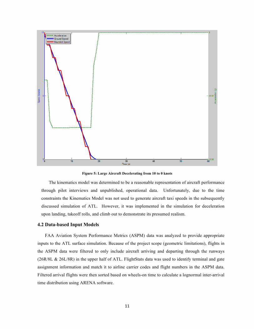
When the model is executed with proper inputs, it yields the output shown in the Figures 4 and 5
below. The data is stored in arrays and the results are plotted on a Cartesian plane. The x-axis
represents time in seconds. The left y-axis represents speed in knots and corresponds to the red and
blue lines. The right y-axis represents the acceleration in g's and corresponds to the green line. The
dotted green line represents the acceleration of the aircraft. This was used for test purposes to ensure
that the acceleration was within acceptable ranges. The blue line represents the ground speed of the
aircraft over time. The red line represents the same data, but rounded to the nearest integer. Figure 4
below shows that approximately 27 seconds are needed for a heavy aircraft to reach a target speed of
10 knots.
Figure 4: Heavy Aircraft Accelerating from 0 to 10 knots
Figure 5 below shows that approximately 19 seconds are needed for a large aircraft to decelerate
from 10 knots to a complete stop.
11
Figure 5: Large Aircraft Decelerating from 10 to 0 knots
The kinematics model was determined to be a reasonable representation of aircraft performance
through pilot interviews and unpublished, operational data. Unfortunately, due to the time
constraints the Kinematics Model was not used to generate aircraft taxi speeds in the subsequently
discussed simulation of ATL. However, it was implemented in the simulation for deceleration
upon landing, takeoff rolls, and climb out to demonstrate its presumed realism.
4.2 Data-based Input Models
FAA Aviation System Performance Metrics (ASPM) data was analyzed to provide appropriate
inputs to the ATL surface simulation. Because of the project scope (geometric limitations), flights in
the ASPM data were filtered to only include aircraft arriving and departing through the runways
(26R/8L & 26L/8R) in the upper half of ATL. FlightStats data was used to identify terminal and gate
assignment information and match it to airline carrier codes and flight numbers in the ASPM data.
Filtered arrival flights were then sorted based on wheels-on time to calculate a lognormal inter-arrival
time distribution using ARENA software.

12
The number of flights for each airline carrier were used to calculate airline probabilities for
subsequently discussed aircraft objects. The number of flights for each airline were identified by a
count of each carrier code throughout each day of interest. Airline probabilities were calculated by
dividing the number of flights for each carrier by the total number of filtered flights for the geometric
region of interest.
To support the kinematics model and attempt to produce realistic variance in the simulation,
probabilities for aircraft type (small, large, heavy) were computed. This was accomplished by
counting the number of aircraft in each weight class and dividing by the total number of filtered
aircraft.
The last input model developed for the ATL simulation is an in gate time distribution. The in gate
time is the difference between the gate-out and gate-in times for an aircraft and varies between
aircraft types, domestic versus international flights, and other factors. Despite derivation of this
probabilistic model, due to time constraints constant values were assumed for each aircraft type,
obtained from consultation of subject matter experts (SMEs) discussed subsequently. These values
were 40 minutes, 60 minutes, and 120 minutes for small, large, and heavy aircraft respectively.
4.3 Atlanta International Surface Simulation
The surface simulation takes inputs from the kinematics model and the data-based input model. It
is controlled by the airport geometry, FAA separation standards to maintain safety, and airline gate
assignments. The model outputs include a plot of surface count per unit time, and a numerical value
for the maximum surface count. It also provides the total and average arrival/departure taxi times.
Development of a simulation for surface operations at for ATL was performed using the process
depicted in Figure 6.
Figure 6: Simulation Development Process
The first step in the process was to identify a portion of the airport geometry that was feasible to
simulate in the time provided and representative of enough of the airport to produce meaningful
results.
4.3.1 Identification of Geometry
A geometry representing nearly half of the airport was determined to be feasible. Dr.
Lance Sherry (the project sponsor) approved this modeling scope. Dr. Alexander Klein, a former

13
GMU SEOR faculty member, was also consulted. Drs. Sherry and Klein are considered to be
subject matter experts (SMEs) with respect to airport surface operations. Dr. Klein developed the
Total Airspace and Airport Modeler (TAAM) tool – an extremely complex and sophisticated
simulation of most airports and airspace in the United States. Drs. Sherry and Klein both
indicated that the upper half of ATL was independent enough of the lower half that results could
be extrapolated to the entire airport.
Using runway dimensions from [4], satellite imagery from Google Maps, and Adobe
Photoshop, a 3.92 meter per pixel relationship was identified and used to obtain measurements for
objects within the identified geometry. These included runways, taxiways, ramps, and gates.
Each measurement was accurate to the aforementioned value of roughly 4 meters. Figure 7
contains a visualization of this step in the development process.
Figure 7: Identification of Geometry
The next step in simulation development process was identification of traffic flows within
the identified feasible geometry.
4.3.2 Identification of Traffic Flows
SMEs were consulted again, regarding traffic flows corresponding to the identified
geometry. Dr. Klein and a post-doctoral CATSR researcher confirmed that a common
configuration for traffic flows is that shown in Figure 8.

14
Figure 8: Identified Traffic Flows
It is important to note that this is not the only traffic flow configuration used at ATL. If
winds shift such that aircraft flowing per Figure 8 encounter significant tail winds, the direction
of arrivals and departures is reversed so that aircraft encounter head winds during landing and
takeoff. Another important consideration is whether one particular flow configuration is
dominant on blue sky days, the periods of interest. Research presented in [1] indicates that blue
sky day congestion can occur with either flow configuration.
This finding is supported by an analysis of Airport Surface Detection Equipment, Model
X, (ASDE-X) multilateration surveillance data for ATL, provided by the SAAB Sensis
Corporation. A MATLAB program was written to input and analyze ASDE-X data for two
known blue sky days (May 3 and 18, 2012) [1]. The MATLAB program reduced the data to only
that for stationary aircraft (ground speed field = 0). Per congestion peaks in [1], three time
periods were examined for each day: morning (09:00 to 11:00 AM Eastern U.S.), afternoon
(02:00 to 4:00 PM Eastern U.S.), and evening (06:00 to 08:00 PM Eastern U.S.).
Stationary aircraft positions were plotted and overlaid upon satellite imagery, producing
the graphic in Figure 9. The majority of congestion on these days, during the three time periods,
occurred on the two parallel taxiways above the ramps and below the departure runway (areas
within boxes in Figure 9).

15
Figure 9: ASDE-X Surveillance Data for Blue Sky Day Congestion
Figure 9 also depicts a departure queue (East-most congestion) for the assumed departure
runway shown in Figure 8. An arrival queue, emanating from the West-most taxiway (below the
assumed arrival runway in Figure 8) is also shown. Observations from the surveillance data
analysis were believed to validate the identified geometry by showing blue sky day congestion
within that geometry. Similarly, these observations appeared to validate the identified traffic
flow configuration with visible arrival and departure queues.
With the identified (and assumed validated) geometry and traffic flow configuration, the
next step in the simulation development process was translation of these characteristics into a
wireframe network model.
4.3.3 Wireframe Network Model
The wireframe network model was developed in distinct steps, in parallel to subsequently
discussed simulation functions, objects, and logic. The model, as it existed at each step, was
rigorously tested, perhaps hundreds of times, until the best possible (time constrained) output was
produced and validated both numerically and visually with a graphical user interface (GUI).
Figure 10 depicts the full wireframe network model overlaid upon runway, taxiway,
ramp, and gate components of the simulation GUI. Nodes are represented by solid blue circles.
Paths between nodes are represented by black lines.

16
Figure 10: Wireframe Network Model for ATL
Each development step included addition of a ramp, starting with the West-most ramp
and ending with the East-most ramp shown in Figure 10. The simulation built upon this network
model is discussed next.
4.3.4 Simulation Environment, Objects, and GUI
The MATLAB environment was selected for this project because of team member
experience and graphical capabilities. The simulation coordinate system is a three dimensional
Cartesian system consisting of x (East/West) and y (North/South) dimensions in the horizontal
plane and a z (altitude) dimension in the vertical plane. The origin (0, 0, 0) is located at the West-
most end of runway 26L.
Data structures were generated for all necessary objects, listed below:
a. Runways
• Occupancy status (0 or 1)
b. Taxiways and ramps
• Defined by node and arc groups
c. Gates
• Defined by nodes
• Number (1 to 92)
• Occupancy status (0 or 1)
d. Aircraft
• Type: small, large, or heavy (probabilistic)
• Airline: 1 for the most common airline at ATL, 2 for the group of all other
airlines operating at ATL (probabilistic)

17
• Flight Identification: ‘ABC’ for airline 1, “OTH” for airline 2; suffix (e.g.
‘001’, ‘002’) is odd for arrivals, even for departures
• x, y, z: position in meters
• xdot, ydot, zdot: velocity in meters per second
• Phase: landing, taxiing in, in gate, taxiing out, taking off
• Time (seconds)
• Time taxiing in (seconds)
• Time taxiing out (seconds)
• Assigned gate number
• Actual gate number
• Last node passed
• Holding status (0 or 1)
The simulation GUI (shown in Figure 11) depicts objects listed above in the horizontal
plane. Additionally, a data block, containing time (in seconds), current surface count, and
maximum surface count, is depicted in upper left corner. Aircraft are represented with “chevron”
(arrow head) symbols per international standards for next generation airborne avionics [7].
Symbols for small aircraft, in this case mostly private and regional jets, are the smallest chevrons
colored green. Symbols for the large aircraft (e.g., Boeing 737, Airbus A320) are colored orange.
Symbols for heavy aircraft (e.g., Boeing 777, Airbus A340) are colored blue and larger than
symbols for large aircraft.
Figure 11: Simulation GUI and Objects

18
The simulation GUI was developed to primarily depict operations in the horizontal plane.
However, vertical behavior (non-zero altitude) is shown with a black symbol depicting a shadow,
painted underneath the corresponding aircraft symbol, but above all other objects; this is
illustrated in more detail in a subsequent section. All simulation objects are controlled with the
functions described in the next section.
4.3.5 Simulation Functional Architecture
The simulation of ATL was designed to be very modular, scalable, and adaptable. The
functional architecture is decomposed in correspondence to the following subsections.
4.3.5.1 Simulate_ATL()
The highest level function declares global variables and contains the following user-
adjustable parameters:
• GUI on/off control flag
• GUI playback speed (e.g., 1 = 1 Hz, 0.1 = 10 Hz)
• Duration (seconds)
• In gate time intervals for each aircraft type (seconds)
• Inter-departure time for all aircraft (seconds)
• Collision threshold or separation distance considered to be a collision (meters);
assumed to be 76.2 meters (250 ft)
This function also initializes all simulation variables and contains a for loop that cycles
through each one second increment of the user-defined duration. Within this for loop, other
functions to generate, land, navigate, separate, hold, and takeoff aircraft are called.
Additionally, computations for outputs (e.g., taxi times, surface count, and maximum surface
count) are performed within this function.
4.3.5.1.1 Generate_aircraft()
This function generates aircraft objects per random inter-arrival times from
lognormal distribution; this parameter is user-adjustable. Aircraft objects are generated
approaching the airport at altitude, horizontally positioned just within the maximum x
value shown in Figure 11. Aircraft type and airline are determined with random uniform
variables obtained from data analysis. Maximum taxi speed, different for each aircraft
type, is set based on values from [8].

19
4.3.5.1.2 Land_aircraft()
This function lands aircraft with an assumed 3 degree glideslope, nominal 130 knot
final approach speed, a touch down point 0.25 nautical miles (463 meters) West of the
arrival runway threshold, and a 0.1g deceleration magnitude (also per [8]) until an aircraft
type specific taxi speed is achieved (prior to the runway end in all cases). Once an
aircraft has exited the runway it is navigated via the wireframe network model.
4.3.5.1.3 Navigate_aircraft()
The highest level navigation function constantly provides instructions to aircraft
objects, at each cycle in the simulation. This function determines gate assignments based
on the assigned airline, gate occupancy, and aircraft location. In most circumstances, the
lowest numbered available gate from the particular airline set is assigned. However, this
function compensates for two corner cases.
In one of these cases, an aircraft receives a gate reassignment after it has entered a
gate leg of the network, but before it has reached the node at the end of that leg (officially
occupying the gate). In this case the reassignment is ignored and the aircraft follows the
previous instruction (encoded in the aircraft object).
In the second case, an aircraft receives a gate reassignment corresponding to a ramp
that it has already passed. Similarly, the reassignment is ignored and the aircraft
continues to the previously assigned ramp. However, in this case the gate assignment
may change based on actions of aircraft ahead.
4.3.5.1.3.1 Navigate_to_ramp()
This navigation sub-function provides arriving aircraft with a precise path to the
assigned ramp in the form of a vector containing all nodes along the path. Aircraft
objects are programmed to keep a history of the last node passed such that they can
perceive the next node at any time. A look ahead algorithm is used to determine
distance to the next node in the path. Once this distance decreases to 10 meters or
less, the aircraft will: continue traveling straight, turn right, or turn left, per fields
indicating this in an object for the next node.

20
4.3.5.1.3.2 Navigate_to_gate()
Similarly, this function provides aircraft with a path to the assigned gate. Once
the look ahead algorithm determines that the assigned gate is directly ahead, aircraft
stop at the gate position and exit the arrival mode.
4.3.5.1.3.3 Navigate_to_runway()
This function provides departing aircraft with a path to the departure runway with
a construct very similar to arrival navigation functions. An aircraft in a gate is set to
the departure mode when its time in the gate exceeds the user-defined in gate interval.
The aircraft flight identifier is incremented by one (converting odd to even). Once an
aircraft reaches the departure runway location, it holds or takes off depending on the
occupancy field in the departure runway object. This occupancy is time-based,
controlled by the user-defined inter-departure time, and reflects the time needed for a
takeoff roll and dissipation of wake vortices generated by departing aircraft.
4.3.5.1.4 Determine_priority_and_detect_conflicts()
This function is the most complex in the simulation and required the most time to
develop. It cycles through pairs of active aircraft on the surface, not landing, in a gate, or
taking off. In many cases, this function simply determines is two aircraft are separated
by a distance less than the user-defined collision threshold; if the threshold is violated one
of the aircraft in the pair is instructed to hold if the other aircraft in the pair is not holding
for it (detected with this same function). This prevents infinite holds from occurring, at
the cost of requiring extremely complex and robust logic to account for all potential
scenarios. Due to time constraints it was admittedly not possible to implement complete
priority and collision avoidance logic. However, the logic in this function does account
for various scenarios, including:
• An algorithm to prevent aircraft entering or leaving neighboring gates from
holds because the distance between the gates is less than the collision
threshold
• A slight priority bias toward arrivals. If a departing aircraft will cross the
path of an arriving aircraft, it will hold unless it is in a position where
holding will significantly impede traffic flow (e.g., in the middle of a ramp).
If the latter occurs the arriving aircraft will temporarily hold for the
departure.

21
• A reward and penalty, first come first serve priority system. For example, if
a later departing aircraft reaches uppermost taxiway before an earlier
departing aircraft because of large disagreement between actual assigned
ramps it will proceed ahead of the earlier departing aircraft.
It is also extremely important to note that this function is responsible for limiting
aircraft taxi speeds based on the type of aircraft it is following. Small aircraft, capable of
greater taxi speeds, will catch up with large and heavy aircraft capable of lower taxi
speeds, but then will be limited to the speed of the aircraft ahead such that the collision
threshold distance is maintained between the aircraft. Similarly, a large aircraft will do
the same when following a heavy. In contrast, if a slower aircraft is a following a faster
aircraft (e.g., heavy behind small or large), an increasing spatial and temporal gap will
form between the two aircraft.
4.3.5.1.5 Hold_aircraft()
This subfunction is responsible for setting the hold status field in aircraft objects, as
determined by its parent function. This function also sets a field in a particular aircraft
object that contains the data structure index of another aircraft it is holding for (to prevent
infinite holds as previously described).
4.3.5.1.6 Takeoff_aircraft()
Once the departure runway occupancy status changes from occupied to unoccupied
per the user-defined inter-departure time, the next aircraft in the departure queue is set to
a takeoff mode. Using the developed kinematics model, aircraft thrust is set to the
maximum level and the aircraft accelerates toward the West along the departure runway.
Thrust to mass ratios for different aircraft types, identified through unpublished analysis
of operational data, were implemented. Once the aircraft reaches takeoff speed (150
knots in this implementation) it climbs until its horizontal position is beyond the
minimum x value shown in Figure 9.
4.3.5.1.7 Paint_display()
If the GUI is enabled by the user, this function is called at each one second time
increment within a simulation run. All GUI objects are refreshed with current states if
depicted. Figure 12 contains sample GUI output for a simulation run containing a
significant number of aircraft. Aircraft can be seen landing on the arrival runway and

22
taking off on the departure runway (shadow depicted). Many occupied gates, several
taxiing aircraft, and departure queue are also visible.
Figure 12: Sample Simulation GUI Output
A 6 minute video demonstration, illustrating roughly 30 minutes of simulated
surface operations (playback roughly 5 times faster than real time), accompanies this
document in MPEG-4 (MP4) format and is available online at the following uniform
resource locator (URL):
https://www.youtube.com/watch?v=glLn8vmlB6s

23
5. Validation, Results, and Sensitivity Analysis
5.1 Validation and Normal Day Results
The ATL surface simulation was validated through experimentation and comparison of output to
known characteristics for a normal, uncongested day. Table 2 contains expected and simulated
results for this scenario, limited to 12 hours (half day) due to time constraints.
Table 2: Expected versus Observed Results for a Normal Half Day.
The expected maximum surface count is an actual observed value (67, morning period [1]) scaled
down by a factor of 3 and rounded to the nearest integer. This was determined through analysis of
surface counts in the upper and lower halves of ATL. The lower half accounts for roughly 2/3 of the
total taxiway count because of a much greater distance between the Southernmost arrival runway and
terminals.
The simulated maximum surface count of 21 (versus expected value of 22) indicates very strong
agreement between output and reality. Expected taxi in and out times were derived from ASPM data
and not scaled or modified in any way. The simulated taxi in time was within 0.5 minutes of the
expected value. The simulated taxi out time was within 1 minute of the expected value.
The ATL simulation was also configured to produce a plot of surface counts versus time for 10
minute periods within the simulation duration. This was used to perform a frequency analysis
depicted by Figure 13.

24
Figure 13: Surface Count versus Time
Simulation time was first aligned with an observed time corresponding to an increase in surface
count. The amplitude of the curve for simulation output was scaled upward by a factor of three,
based on the previously discussed rationale and assumption that results can be extrapolated to the
entire airport. This does, however, limit the meaningfulness of an amplitude comparison. Despite
this, an 8 hour segment of the simulated period (dashed box) is remarkably close to the observations
both in trend and finer oscillations. This is not believed to be a coincidence. Subsequent
disagreement beyond the 8 hour simulation segment is postulated to be caused by simulation
limitations (discussed subsequently).
5.2 Blue Sky Day Results
The simulation was configured to run 12 hours (half) of a blue sky. This simply consisted of a
10 second (7.6%) reduction to inter-arrival times to produce banks of early arrivals. The marginal
change in configuration is due to logic limitations that do not support confidence in results for
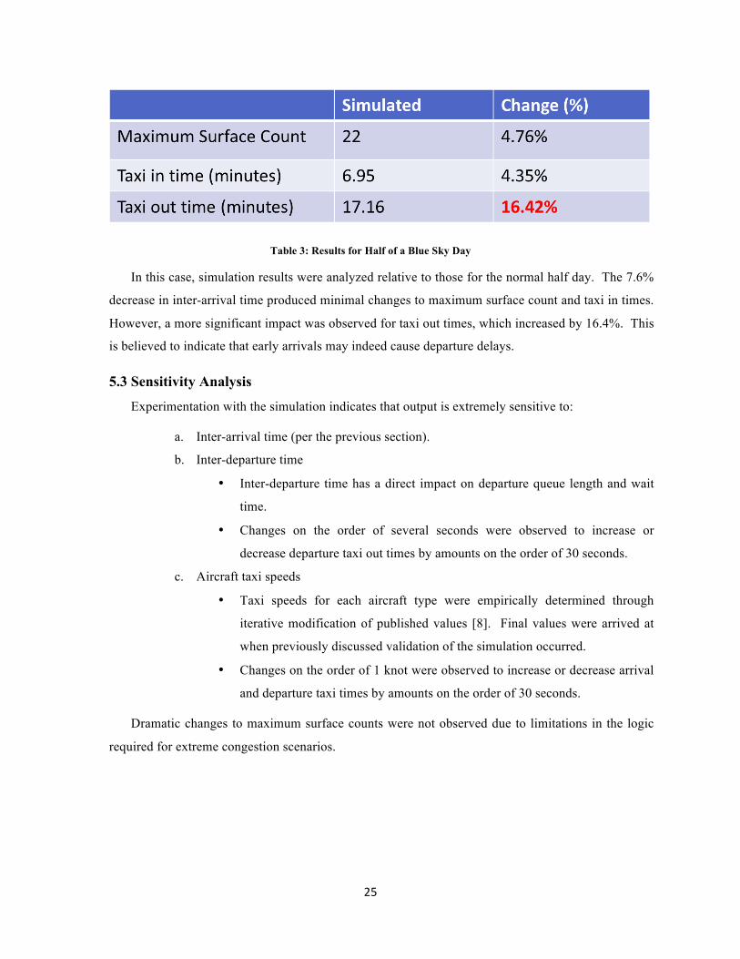
extremely congested scenarios. Table 3 contains results for a minimally congested scenario.
25
Table 3: Results for Half of a Blue Sky Day
In this case, simulation results were analyzed relative to those for the normal half day. The 7.6%
decrease in inter-arrival time produced minimal changes to maximum surface count and taxi in times.
However, a more significant impact was observed for taxi out times, which increased by 16.4%. This
is believed to indicate that early arrivals may indeed cause departure delays.
5.3 Sensitivity Analysis
Experimentation with the simulation indicates that output is extremely sensitive to:
a. Inter-arrival time (per the previous section).
b. Inter-departure time
• Inter-departure time has a direct impact on departure queue length and wait
time.
• Changes on the order of several seconds were observed to increase or
decrease departure taxi out times by amounts on the order of 30 seconds.
c. Aircraft taxi speeds
• Taxi speeds for each aircraft type were empirically determined through
iterative modification of published values [8]. Final values were arrived at
when previously discussed validation of the simulation occurred.
• Changes on the order of 1 knot were observed to increase or decrease arrival
and departure taxi times by amounts on the order of 30 seconds.
Dramatic changes to maximum surface counts were not observed due to limitations in the logic
required for extreme congestion scenarios.

26
6. Known Issues (Limitations) and Potential Future Work
Known issues include the following:
a. Aircraft hold logic for extreme congestion scenarios contains gaps because of time
constraints.
b. An observed phenomenon – aircraft temporarily parking behind occupied gates when all
gates are full – was not fully implemented, also because of time constraints.
These issues form the rationale for the limited analysis of blue sky day congestion; the congestion
level could only be marginally increased for this study. It is estimated that a task to correct the first item
above will require roughly 3 to 4 weeks. The second item above is estimated to require roughly 2 to 3
weeks of work.
Future work includes a more detailed analysis of blue sky days and determining the feasibility of
implementing various surface management techniques to Hartsfield-Jackson Atlanta International Airport.
7. Conclusions and Recommendations
A simulation of Hartsfield-Jackson Atlanta International Airport (ATL) was developed through
systems engineering processes. These processes included design, integration, testing, experimentation,
analysis, and validation. An analysis of surface counts, arrival taxi in times, and departure taxi out times
for a normal day indicate that the simulation is a reasonably accurate representation of the upper half of
the airport. The ATL simulation, configured for a normal day, is believed to accurately represent nominal
surface operations as shown through experimentation, analysis, and validation. A limited analysis of blue
sky days indicates that banks of early arrivals may indeed be the cause of departure delays.
A tangible product (MATLAB M file) accompanies this paper and is available to GMU faculty and
others at their discretion. The models and simulation developed for this project are:
a. Scalable for additional objects (e.g., taxiways, runways, runway exits, ramps, gates, etc.)
b. Adaptable for other airport geometries (no limitation to ATL)
c. Easily improved upon with additional time
d. A good candidate for future student projects, although this is recommended for the graduate level
It is recommended that work on this project is continued and further analysis of blue sky days is to be
conducted. With a reasonable amount of effort a more detailed and accurate analysis of blue sky days is
likely possible. Additionally, incorporation of a more complete geometry will strengthen capabilities of
the simulation and provide results more applicable to the entire airport. The ATL simulation, configured

27
for a normal day, is believed to accurately represent nominal surface operations as shown through
experimentation, analysis, and validation.
8. Acknowledgments
The authors would like to give special acknowledgement to several individuals who contributed to
this project:
• Dr. Lance Sherry
− Project Sponsor, George Mason University (GMU) Center for Air Transportation
Systems Research (CATSR)
• Dr. Kathryn Laskey
− Graduate Capstone Course Instructor and Faculty Advisor, George Mason University
(GMU) Department of Systems Engineering & Operations Research (SEOR)
• Dr. Alexander Klein
− Senior Vice President of Research & Development, AvMet Applications
• Dr. Benjamin Levy
− Manager, Operations Research Group, the SAAB Sensis Corporation
• Mr. Peter Stassen
− Principal Engineer and Pilot, the MITRE Corporation.
9. References
[1] Neyshabouri, S., 2013, Analysis of Airport Surface Operations: a Case Study of Atlanta Hartsfield
Airport, Fairfax, VA, George Mason University.
[2] Federal Aviation Administration, 2014, Aviation System Performance Metrics Database, available:
http://aspm.faa.gov/main/aspm.asp
[3] Stroiney, S., B. Levy, 2011, Departure Queue Management Benefits Across Many Airports,
Proceedings of the 2011 Integrated Communications Navigation and Surveillance (ICNS) Conference,
Herndon, VA, IEEE.
[4] AirNav LLC, 2014, KATL - Hartsfield - Jackson Atlanta International Airport, available:
http://www.airnav.com/airport/KATL
[5] Federal Aviation Administration, 2013, Airport Diagram: Hartsfield - Jackson Atlanta International,
Washington, DC, U.S. Department of Transportation.
[6] Sherry, L., 2011, Aircraft Performance, Fairfax, VA, George Mason University.

28
[7] RTCA Special Committee 186, 2014, Minimum Operational Performance Standards (MOPS) for
Aircraft Surveillance Applications (ASA) System, DO-317B, Washington, D.C., RTCA Inc.
[8] Ravizza, S., et al., 2012, The Trade-off Between Taxi Time and Fuel Consumption in Airport Ground
Movement, Conference on Advanced Systems for Public Transport (CASPT12), Santiago, Chile.
29
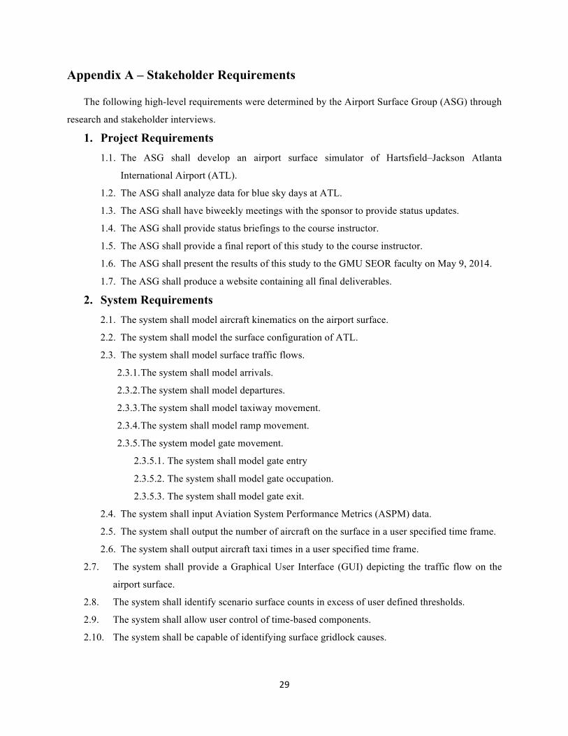
Appendix A – Stakeholder Requirements
The following high-level requirements were determined by the Airport Surface Group (ASG) through
research and stakeholder interviews.
1. Project Requirements 1.1. The ASG shall develop an airport surface simulator of Hartsfield–Jackson Atlanta
International Airport (ATL).
1.2. The ASG shall analyze data for blue sky days at ATL.
1.3. The ASG shall have biweekly meetings with the sponsor to provide status updates.
1.4. The ASG shall provide status briefings to the course instructor.
1.5. The ASG shall provide a final report of this study to the course instructor.
1.6. The ASG shall present the results of this study to the GMU SEOR faculty on May 9, 2014.
1.7. The ASG shall produce a website containing all final deliverables.
2. System Requirements 2.1. The system shall model aircraft kinematics on the airport surface.
2.2. The system shall model the surface configuration of ATL.
2.3. The system shall model surface traffic flows.
2.3.1. The system shall model arrivals.
2.3.2. The system shall model departures.
2.3.3. The system shall model taxiway movement.
2.3.4. The system shall model ramp movement.
2.3.5. The system model gate movement.
2.3.5.1. The system shall model gate entry
2.3.5.2. The system shall model gate occupation.
2.3.5.3. The system shall model gate exit.
2.4. The system shall input Aviation System Performance Metrics (ASPM) data.
2.5. The system shall output the number of aircraft on the surface in a user specified time frame.
2.6. The system shall output aircraft taxi times in a user specified time frame.
2.7. The system shall provide a Graphical User Interface (GUI) depicting the traffic flow on the
airport surface.
2.8. The system shall identify scenario surface counts in excess of user defined thresholds.
2.9. The system shall allow user control of time-based components.
2.10. The system shall be capable of identifying surface gridlock causes.

30
Appendix B – Project Management
B.1 Work Breakdown Structure
A Work Breakdown Structure (WBS), depicted in Figure 14, was developed to assist in planning,
evaluating, and managing project tasks. The WBS has been decomposed into five components:
project management, deliverables, front end analysis, back end analysis and development, and
solution. Project management consists of planning, team meetings, Earned Value Management
(EVM), and sponsor evaluations. The purpose of these tasks is to ensure the project team remains
focused on sponsor needs, within budget, and on time. Deliverables include status briefings, written
reports a project website, and peer evaluations. The front end analysis consists of research, problem
definition, scope determination, and requirements formulation. It also includes data analysis, which is
critical for the back end analysis and development that encompasses the design, coding, and testing of
the software. The solution includes analysis of results and group recommendations for the problem.
Airport Surface Congestion Project
3.0 Front End
4.0 Back End
2.0 Deliverables
5.0 Solution
1.0 Project Management
1.2 Team Meetings
1.3 Earned Value Management
2.1 Presentations
2.3 Website
2.2 Reports
3.1 Context
3.2 Problem Definition
3.3 Scope Definition
3.4 Requirements Formulation
4.2 Development / Coding
4.1 Design
4.3 Testing
3.5 Data Analysis
5.1 Analysis of the Results
2.4 Peer Evaluations
1.1 Planning
1.4 Sponsor Evaluation
Figure 14: Work Breakdown Structure

31
B.2 Schedule
The project schedule was implemented as a Gantt chart as shown in Figure 15. The schedule was
set to 16 weeks. The duration of each task in the WBS was estimated. The project progress was
tracked throughout the semester using EVM.
Figure 15: Schedule & Gantt Chart

32
B.3 Earned Value Management
Figure 16 shows the earned value of the project over its entire duration. The budgeted cost of
work performed and actual cost of work performed are seen to remain roughly consistent with the
expected costs throughout the duration of the project. In the graph the red line represents the projected
budget, which was set according to our baseline plan, the green line shows the actual cost and the
blue represents the earned value. These values only outline the project current status up to week 15 of
2014.
Figure 16: Earned Value Over Time
The Cost Performance Index (CPI) and Schedule Performance Index (SPI) indicate how closely
the accomplished work is on budget and within schedule. The CPI and SPI indices are only
showcasing the project update until Week 15 as shown in figure 17. According to the figure, the
project was on schedule, but more hours were needed to accomplish the tasks. Therefore, the project
went above the estimated cost with a cost variance of approximately 37k.

33
Figure 17: Cost & Schedule Performance Indices Over Time
B.4 Risks and Mitigations
There were several risks involved in the project. Table A1 below describes each risk as well as
the severity and mitigation strategy for that risk.
Table 4: Risks & Mitigations
ID Risk Severity Mitigation
1 Failure to complete a
simulation of the entire airport
due to time constraints.
High Based on meetings with SMEs, the airport has
two control towers, each controlling half of the
airport. A simulation of the upper half of the
airport will most likely provide reliable results.
2 Failure to integrate the
kinematics and network
models
Medium Use constant speeds for each aircraft type.
3 Failure to verify and analyze
the models.
Medium Allocate time for testing and analysis in order to
show the capability and results of the work
accomplished.
4 Having incompatible code that
makes the models difficult to
integrate.
Small Attempt to implement all of the models and code
in a single environment (MATLAB) for easier
integration.


![Airport Surface Operation Collaborative Automation Concept · important factor affecting airport operations, the Dallas – Fort Worth (DFW) Airport Development Plan [10] includes](https://img.dokumen.tips/doc/110x75/5f77025e5092e0635c33d742/airport-surface-operation-collaborative-automation-important-factor-affecting-airport.jpg)


![[EN Results of Airport Surface Multilateration[EN105] Evaluation Results of Airport Surface Multilateration ... ENRI Int. Workshop on ATM/CNS. Tokyo, Japan. (EIWAC 2010) Figure 10](https://img.dokumen.tips/doc/110x75/5e8a63671cf60f29276daff1/en-results-of-airport-surface-multilateration-en105-evaluation-results-of-airport.jpg)