Science of the Total Environment 485–486 (2014) 62–70

Contents lists available at ScienceDirect

Science of the Total Environment

j ourna l homepage: www.e lsev ie r .com/ locate /sc i totenv

A network-based approach for estimating pedestrian journey-timeexposure to air pollution

Gemma Davies ⁎, J. Duncan WhyattLancaster Environment Centre, Lancaster University, Lancaster, Lancashire, LA1 4YQ, UK

H I G H L I G H T S

• Physiology and activity level incorporated into estimates of journey-time exposure• Easy comparison of exposure between multiple origins and destinations• Flexibility to compare exposure between different individuals for different days• Ability to assess alternate ‘least exposed’ alternatives

⁎ Corresponding author. Tel.: +44 1524 510252.E-mail addresses: gemma.davies@lancaster.ac.uk (G. D

d.whyatt@lancaster.ac.uk (J.D. Whyatt).

http://dx.doi.org/10.1016/j.scitotenv.2014.03.0380048-9697/© 2014 Elsevier B.V. All rights reserved.

a b s t r a c t

a r t i c l e i n f o

Article history:Received 31 October 2013Received in revised form 4 March 2014Accepted 10 March 2014Available online 3 April 2014

Editor: Lidia Morawska

Keywords:PM2.5

Journey-time exposureAir pollution modellingGIS network analysisPhysiology

Individual exposure to air pollution depends not only upon pollution concentrations in the surrounding environ-ment, but also on the volume of air inhaled, which is determined by an individual's physiology and activity level.This study focuses on journey-time exposure, using network analysis in a GIS environment to identify pedestrianroutes betweenmultiple origins and destinations throughout the city of Lancaster, NorthWest England. For eachsegment of a detailed footpath network, exposurewas calculated accounting for PM2.5 concentrations (estimatedusing an atmospheric dispersion model) and respiratory minute volume (varying between individuals and withslope). For each of the routes generated the cumulative exposure to PM2.5 was estimated, allowing for easycomparison between multiple routes.Significant variations in exposure were found between routes depending on their geography, as well as in re-sponse to variations in background concentrations and meteorology between days. Differences in physiologicalcharacteristics such as age or weight were also seen to impact journey-time exposure considerably. In additionto assessing exposure for a given route, the approach was used to identify alternative routes that minimisedjourney-time exposure. Exposure reduction potential varied considerably between days, with even subtle shiftsin route location, such as to the opposite side of the road, showing significant benefits.The method presented is both flexible and scalable, allowing for the interactions between physiology, activitylevel, pollution concentration and journey duration to be explored. In enabling physiology and activity level tobe integrated into exposure calculations a more comprehensive estimate of journey-time exposure can bemade, which has potential to provide more realistic inputs for epidemiological studies.

© 2014 Elsevier B.V. All rights reserved.

1. Introduction

Evidence indicates that transport-related air pollution has a numberof health implications including mortality (Heinrich et al., 2005). Theseinclude short-term effects such as irritation to eyes, nose and throat,upper respiratory infections, headaches, nausea and allergic illnesssuch as asthma. Long term effects include chronic respiratory disease,cancer, heart disease and even brain damage. Ambient air pollution

avies),

has also been linked with low birth weight (Xia and Tong, 2006;Heinrich et al., 2005; Krzyzanowski, 2005; RCEP, 2007; Pedersen et al.,in press). Health impacts from transport-related air pollutionmay occur in response to a single journey (McCreanor et al., 2007;Peters et al., 2004). Reducing exposure to transport-related air pollutionis therefore a key target for public health (RCEP, 2007; Künzli et al.,2000).

An individual's exposure to air pollution depends on the duration ofexposure and volume of pollutants inhaled (Xia and Tong, 2006).Inhalation rates depend on both an individual's physiology and activitylevel. The main atmospheric pollutants affecting public health includenitrogen dioxide (NO2), particulates, sulphur dioxide (SO2) and ozone

63G. Davies, J.D. Whyatt / Science of the Total Environment 485–486 (2014) 62–70

(O3) (Xia and Tong, 2006). Of these, particulates have the longest cumu-lative effect on health as they contain materials not easily digested andresolved by the body, and can be deposited in the nose, throat and lungs(Xia and Tong, 2006). This study will therefore concentrate on particu-late matter less than 2.5 μm in diameter (PM2.5) as other researchershave shown that these are of greatest concern for human health (Popeand Dockery, 2006; Schwartz and Neas, 2000). PM2.5 is a non-threshold pollutant, with health impacts potentially occurring evenwith low concentrations (RCEP, 2007; Pope and Dockery, 2006).

While the proportion of an individual's time spent in transit is rela-tively small it can account for a disproportionately high amount oftheir exposure to air pollution. The impact of journey-time exposureon health is therefore potentially significant (Gulliver and Briggs,2005). For example, when evaluating personal exposure to black car-bon, Dons et al. (2012) found that while only 6.3% of participant timewas spent in transport, this corresponded to 21% of their personal expo-sure. Some studies have sought to calculate journey-time exposureusing monitoring (Yu et al., 2012; Gómez-Perales et al., 2004; Chanet al., 2002); however this approach is necessarily limited in the numberof potential routes for which exposure estimates can be determined.Attempts have been sought to address this challengemodelling bothpol-lutant concentrations and potential route choices (Gulliver and Briggs,2005; Hertel et al., 2008). However, very little research into journey-time exposure accounts for physiology and activity level despite theirsignificance in influencing individual exposure (inhaled dose). Oneexception to this is the work by Int Panis et al. (2010) who recognisethe importance of considering inhaled dose when comparing exposurebetween cyclists and car passengers, using monitoring techniques torecord particulate concentrations and respiratory measurements.

Fig. 1.Modelled factors affecting journ

However, consideration of respiratory rates remains conspicuously ab-sent from most other studies.

The aim of this paper is to present a method for calculating journey-time exposure between any combination of origins and destinations, in-corporating not only duration of journey and pollution concentrationsas considered by Gulliver and Briggs (2005), but accounting also forphysiology and activity level, thus enabling exposure to be calculatedas inhaled dose (μg) rather than ambient exposure (μg m−3). Thisstudy will focus entirely on pedestrians and hence consider only out-door exposure; however, the same approach could be applied to othertransport modes, or multimodal networks. In considering pedestriansonly, the range of activity levels to be considered is reduced and theneed to scale pollutant concentrations for different transport modes isavoided. Typically ‘in vehicle’ modes of transport are associated withlower activity levels than walking or cycling and therefore lower respi-ratory rates and potentially lower inhaled dose. This, however, needs tobe balanced against the potential health benefits of increased activitylevels (de Hartog et al., 2010). As exposure generally peaks duringpeak commuting hours (Briggs, 2005; Dons et al., 2013) the case studypresented focuses on 08:00 to 09:00 in the morning, with traffic flowdata representing typical rush hour conditions. The method will alsobe applied to explore the potential to reduce journey-time exposureby determining routes of least exposure in addition to fastest routes.The network developed for the purpose of this analysis includes foot-paths on either side of main roads, thus enabling the contrast in expo-sure between different sides of the road to be considered (Greaveset al., 2008).

This paper demonstrates the application of network analysis withina Geographic Information System (GIS) to calculate walking routes

ey-time exposure to air pollution.

Table 1Time impedance for crossing roads.

Crossing type Time impedance (s)

Traffic island 5Traffic island on busy road sections 10Zebra crossing 15Pedestrian lights 25Pedestrian lights as part of traffic control 45Additional crossing points 30Additional crossing points on busy road sections 80

64 G. Davies, J.D. Whyatt / Science of the Total Environment 485–486 (2014) 62–70

through a path network. The analysis incorporates journey duration(minutes); modelled PM2.5 concentrations (μg m−3); and respiratoryminute volume (VE) as a measure of physiology and activity level.Combined, these three elements enable the estimation of journey-time exposures under varying meteorological and backgroundconditions. Fig. 1 summarises the wide range of factors which influencejourney-time exposure andwhich are accounted for within themethodpresented.

2. Methods

This case study focuses on the city of Lancaster, NorthWest England,which has a population of approximately 55,000. While there are nomajor air pollution problems in Lancaster, an air quality management

Fig. 2. Study area

area has been declared around the main gyratory system where trafficcongestion frequently occurs during peak hours—this is illustrated inFig. 2.

, Lancaster.

Table 2Variation in walking speed with slope.

Gradient (°) Uphill speed (km/h) Downhill speed (km/h)

0–4.5 5.0 5.04.5–6.5 5.5 5.76.5–7.5 5.0 5.2N7.5 4.6 4.7

Box 1Calculations for respiratory minute volume.

Calculating Respiratory Minute Volume (VE)

Step 1 Harris Benedict equation for resting metabolic rate(RMR) (kcal.day−1):

Male ¼ 66:4730þ 5:0033Hþ 13:7516W−6:7550AFemale ¼ 65:0955þ 1:8496Hþ 9:5634W−4:6756A

Step 2 kcal.day−1 converted to ml.kg−1.min−1, using thefollowing formula:

kcal:day−1=1440 ¼ kcal:min−1;kcal:min−1=5 ¼ L:min−1;L:min−1=w� 1000 ¼ ml:kg−1:min−1

Step 3

CorrectedMET ¼ MET� 3:5 ml:kg−1:min−1HarrisBenedictRMR ml:kg−1:min−1ð Þ

Step 4

VEm3:min−1 ¼ CorrectedMET� V=1000

Equations taken from Ainsworth (2011)Height and weights from Halls and Hanson (2008).Ventilation rate from Berne et al (2004)

H ¼ height cmð Þ male ¼ 178cm; female ¼ 164cm½ �W ¼ weight kgð Þ male ¼ 70kg; female ¼ 60kg½ �A ¼ age yearð Þ 25 years old½ �V ¼ ventilation rate litres per minuteð Þ 6 L:min−1� �

65G. Davies, J.D. Whyatt / Science of the Total Environment 485–486 (2014) 62–70

2.1. The network dataset

The network dataset was created using a selection of OrdnanceSurvey (OS) digital map data (MasterMap product). Local streets,pedestrianised streets, alleys and private roads (with public access)were taken directly from the Integrated Transport Network (ITN)layer, with the routes represented as a single centre line. For busierroads the pavements on either side of the road were captured usingthe MasterMap Topography layer to determine the distance betweenthe pavement and road centreline. This enabled exposure comparisonsfor opposite sides of a road to be incorporated into the analysis. Addi-tional known footpaths including the canal tow path were also addedto the network, resulting in a comprehensive footpath network accurateto +/−1 m.

Where both sides of the road were captured separately, road cross-ing locations needed to be incorporated into the network. Google StreetViewwas used to identify the location and type of pedestrian crossingson main roads within the study area. Additional crossing points wereadded at further locations where the provision of specified pedestriancrossing points was limited (as quiet local streets are represented by asingle road centreline this assumes no time for crossing roads). For busi-er roads time impedances for crossingwere assumed as listed in Table 1.The crossing impendances were estimated from field observation andinformation from the local authority regarding the phasing of trafficlights.

For the purpose of this analysis a typical walking speed of 5 kphwasassumed (Colclough andOwens, 2010). The impact of gradient onwalk-ing speeds was also calculated. Directional-dependent slope was calcu-lated for each segment of the network, first ensuring that no networksegment was greater than 50 m in length to reduce the likelihood ofmultiple changes in slope direction. Walking speeds were assigned tonetwork segments as shown in Table 2 (Finnis and Walton, 2007 andColclough and Owens, 2010).

2.2. Respiratory minute volume

Physiology and activity level are represented in the analysis throughthe calculation of respiratory minute volume (VE). When combinedwith PM2.5 concentrations and duration of exposure, VE can be used tocalculate exposure in terms of inhaled dose. VE is calculated formetabol-ic equivalents (MET) representing varying activity levels with slope, atthe assumed walking speeds already defined. The METs were takenfrom Ainsworth et al. (2011) and are summarised in Table 3.

To calculate VE from METs, ‘corrected’ METs were calculated formales and females aged 25, of average weight and height (Halls andHanson, 2011). The average of the corrected METs for 25 year oldmales and femaleswas used in the analysis. These were thenmultipliedby a typical resting ventilation rate of 6 l per minute (Berne et al., 2004)

Table 3MET and VEs.

Activity level MET VE

Walking 4.5–5.1 km/h 3.5 0.022Walking 4.7–5.6 km/h, 3.6–20° slope 5.3 0.033Walking 4.7–5.6 km/h, greater than 20° slope 8.0 0.050

to calculate a baseline VE for use in the analysis. The calculations for VE

are shown in Box 1.

2.3. Modelling PM2.5 concentrations

PM2.5 concentrations were modelled using the dispersion modelADMS Urban v.3 (CERC, 2010). ADMS Urban is a comprehensive atmo-spheric dispersionmodelling system,which is used across theworld forstudies of air quality within urban areas and is suitable for use fromstreet level to city-wide scales, accounting for a range of pollutionsources (CERC, 2013). For this study an emissions inventory was de-rived from point sources listed in the NAEI emissions inventory for2011 (DEFRA, 2011) and road traffic emission estimates calculatedfrom road traffic counts, speeds and vehicle composition, with trafficdata obtained from the local authority, Lancashire County Council. Theavailable traffic count data comprised a mix of continuous traffic coun-ters (used for long term traffic monitoring), and automatic traffic countdata (typically covering the period of a week and collected for specificpurposes such as planning applications). These counts were supple-mented where available with annual average daily flow (AADF) trafficcounts (DFT, 2011). The dates for available data varied, with recordschosen from the available data which most closely represented typicalmorning rush hour (08:00–09:00) for the year 2011. Traffic flow andcomposition data were assigned to road centrelines from the OSMasterMap ITN layer, which were then imported to ADMS-Urban torepresent road sources. The latest road source emission factor dataset

66 G. Davies, J.D. Whyatt / Science of the Total Environment 485–486 (2014) 62–70

UK EFT v4.2 was utilised within the model (CERC, 2010). Canyons weremodelled for sections of the main gyratory around the city centre,where the road is surrounded by tall buildings on either side. The can-yon widths were measured from the MasterMap Topography layer,and heights for surrounding buildings calculated from LiDAR data.

Meteorological datawere taken fromManchester Ringwaymeteoro-logical station (BADC, 2012) (45 miles south east of Lancaster). Back-ground PM2.5 data were obtained from DEFRA's air quality dataarchive (http://uk-air.defra.gov.uk/data/) for the urban backgroundmonitoring site for Preston (20 miles south of Lancaster). Due to miss-ing records, the months of March and September were taken as beingbroadly representative of the range ofmeteorological conditions experi-enced throughout 2011.

Themodel was run to a set of 234,563 receptors spaced at 2m inter-vals along each line segment in the network. The average PM2.5 concen-tration per line segment was subsequently calculated for the period08:00 to 09:00 h and assigned to each line segment in the path network.

2.4. Exposure calculation

Slope for each line segment was calculated from the length of theline segment and the difference in elevation between its start and endpoints. For both uphill and downhill directions the duration in minuteswas calculated from the length and the appropriate speed as definedearlier in Table 2. Appropriate VE rates were also assigned to uphilland downhill directions for each line segment relative to the slope.From these attributes exposure to PM2.5 in both uphill and downhill di-rections was calculated for every line segment in the path networkbased on the equation:

Exposure μgð Þ ¼ MeanPM2:5 μg:m−3� �� Duration minutesð Þ� VE m3:min−1� �

2.5. Network analysis

Network analysis was carried out using the network analyst exten-sion within ArcGIS 10 (ESRI, 2010) Network attributes were createdboth for the duration in minutes and the exposure to PM2.5 for each ofthe 60 sample days in the study. This enables either fastest, or least pol-luted routes to be computed from any origin to any destination withinthe study area on any given day. For each route the accumulated timeand PM2.5 exposure is calculated.

5 10 15 200

10,000

20,000

30,000

40,000

50,000

60,000

70,000

80,000

90,000

100,000

Journey-tim

Fre

quen

cy

Fig. 3. Journey-time exposure distribution for all route combinations and da

In addition to calculating individual routes, origin destination (OD)cost matrixes were used to compute journey time exposure for numer-ous routes throughout the city, from each postcode centroid (whichtypically represents around 15 addresses (ONS, 2012)), to a set of 12destinations shown in Fig. 2, which represent the main secondary andtertiary education providers, key employers such as the city counciland hospital, and the major public transport hubs within the city. ODcost matrixes are used to compute and store the fastest or least pollutedpath between multiple combinations of potential route origins (startpoints) and destinations (end points). While OD cost matrices do notdisplay the routes chosen they are able to generate accumulated PM2.5

exposure for hundreds of potential routes, limited only by the numberof origins and destinations required and the size and quality of the net-work dataset. They therefore enable a broader analysis of the variationin potential journey-time exposure across the city.

The analysis was run first to demonstrate its application in assessingjourney time exposure, assuming fastest routes between origin and des-tination were chosen. Routes designed to minimise exposure to PM2.5

were also generated.

3. Case study results

Journey-time exposures were calculated for 60 days, from 1370 ori-gins (unit postcodes) to 12 destinations, giving a total of 986,400 routecalculations. From this, journeys with durations of less than 2 min orgreater than 25 min were excluded from further analysis. Short jour-neys were excluded because total exposure and potential for exposurereduction were likely to be very small. Longer journeys were excludedbecause it was felt that people would adopt alternative forms of trans-port in preference to walking. This left 530,100 route combinations forfurther analysis; the distribution of these relative to journey-time expo-sure can be seen in Fig. 3. The mean journey-time exposure to PM2.5

when walking along routes designed to minimise duration of journeywas calculated as 6.59 μg, with an understandably strong relationshipbetween the average journey-time exposure for a given route and theduration of the journey along that route (r2 = 0.976). This strongrelationship, however, masks considerable variation between days aswell as between routes. On average the range between minimum andmaximum exposure for a single route over the 60 days modelled was24 μg, with exposure varying by up to 44 μg for longer routes(c.25 min). Variation between days is strongly governed by variationin background PM2.5 concentrations, and associated meteorologicalconditions. The journey-time exposure data presented in Fig. 3 is posi-tively skewed towards journeys with relatively low exposure to PM2.5;

25 30 35 40 45

e exposure (µg)

ys modelled within the study, assuming minimising journey duration.

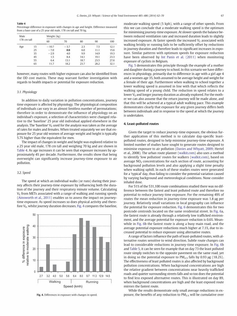
Table 4Percentage difference in exposure with changes in age and height. Difference measuredfrom a base case of a 25 year old male, 178 cm tall and 70 kg.

Male178 cm tall

Weight (kg)

60 70 80 90 100

Age 15 −10.7 −3.7 2.3 7.5 12.125 −7.0 0.0 6.0 11.1 15.635 −2.9 4.0 9.9 14.9 19.345 1.5 8.4 14.1 19.1 23.355 6.4 13.1 18.7 23.5 27.665 11.7 18.2 23.7 28.2 32.1

67G. Davies, J.D. Whyatt / Science of the Total Environment 485–486 (2014) 62–70

however, many routes with higher exposure can also be identified fromthe OD cost matrix. These may warrant further investigation withregards to health impacts or potential for exposure reduction.

3.1. Physiology

In addition to daily variation in pollution concentrations, journeytime exposure is affected by physiology. The physiological compositionof individuals can vary in an almost limitless number of permutations;therefore in order to demonstrate the influence of physiology on anindividual's exposure, a selection of characteristics were changed rela-tive to the ‘baseline’ 25 year old individual applied elsewhere in theanalysis. The ‘baseline’ VE used for the analysis was taken as the averageof rates for males and females. When treated separately we see that ex-posure for 25 year old women of average weight and height is typically5.7% higher than the equivalent for men.

The impact of changes in weight and height was explored relative toa 25 year old male, 178 cm tall and weighing 70 kg and are shown inTable 4. As age increases it can be seen that exposure increases by ap-proximately 4% per decade. Furthermore, the results show that beingoverweight can significantly increase journey-time exposure to airpollution.

3.2. Speed

The speed at which an individual walks (or runs) during their jour-ney affects their journey-time exposure by influencing both the dura-tion of the journey and their respiratory minute volume. CalculatingVE from METs associated with a range of walking and running speeds(Ainsworth et al., 2011) enables us to assess the impact on journey-time exposure. As speed increases so does physical activity and there-fore VE, whilst journey duration decreases. Fig. 4 compares the baseline,

Fig. 4. Differences in exposure with changes in speed.

moderate walking speed (5 kph), with a range of other speeds. Fromthis we can conclude that a moderate walking speed is the optimumforminimising journey-timeexposure. At slower speeds the balance be-tween reduced ventilation rate and increased duration leads to slightlyincreased exposure. At faster speeds the increased VE associated withwalking briskly or running fails to be sufficiently offset by reductionsin journey duration and therefore leads to significant increases in expo-sure. Similar patterns with optimum speeds for exposure reductionhave been observed by Int Panis et al. (2011) when monitoringexposure of cyclists in Belgium.

Fig. 5 demonstrates this principle through the example of a motherand daughter during a journey to school. In this scenario we have differ-ences in physiology, primarily due to difference in age with a girl age 4and awomen age 35, both assumed to be average height andweight fora female of their age. Furthermore when walking to school together alower walking speed is assumed in line with that which reflects thewalking speed of a young child. The reduction in speed relates to alower VE and longer journey duration as already explored. For themoth-er we can also assume that the return journey will be made alone, andthat this will be achieved at a typical adult walking pace. This exampledemonstrates clearly that exposure for any given journey differs bothbetween individuals and in response to the speed at which the journeyis undertaken.

4. Least-polluted routes

Given the target to reduce journey-time exposure, the obvious fur-ther application of this method is to calculate day-specific least-polluted routes, designed to help minimise journey-time exposure. Alimited number of studies have sought to generate routes designed tominimise exposure to air pollution (Davies and Whyatt, 2009; Hertelet al., 2008). The urban route planner (walkit.com) also uses a methodto identify ‘low pollution’ routes for walkers (walkit.com), based onaverage NO2 concentrations for each section of route, accounting forbackground pollution levels and also applying a slight time penaltywhen walking uphill. In each of these studies routes were generatedfor a ‘typical’ day, thus failing to consider the potential variation causedby varying background and meteorological conditions. None considerinhaled dose.

For 51% of the 531,100 route combinations studied there was no dif-ference between the fastest and least polluted route and therefore nopotential to reduce journey time exposure. For the remaining 49% ofroutes the mean reduction in journey-time exposure was 1.8 μg perjourney. Relatively small variations in local geography can influencethe potential for exposure reduction. Fig. 6 demonstrates this for twopostcode centroids located on the same residential street. In Fig. 6a,the fastest route is already through a relatively low trafficked environ-ment, and the average potential for exposure reduction is 0.6%. Mean-while in Fig. 6b the fastest route is along a busy main road, and theaverage potential exposure reductions much higher at 7.1%, due to in-creased potential to reduce exposure using alternative routes.

A range of factors influence the path of least-polluted routes,with al-ternative routes sensitive to wind direction. Subtle route changes canlead to considerable reductions in journey-time exposure. In Fig. 6band Table 5, it can be seen for example that on day 73 the least pollutedroute simply switches to the opposite pavement on the same road, yetin doing so the potential exposure to PM2.5 falls by 0.93 μg (18.2%).The effectiveness of least polluted routes is also affected by backgroundpollution concentrations. When background concentrations are highthe relative gradient between concentrations near heavily traffickedroads and quieter surrounding streets falls and so too does the potentialto find less exposed alternative routes. This is illustrated on day 89,when background concentrations are high and the least exposed routemirrors the fastest route.

While the results demonstrate only small average reductions in ex-posure, the benefits of any reduction to PM2.5 will be cumulative over

0 100 200 Metres

Home

School

Walking Speed (kmh-1)

Duration (minutes)

PM2.5 exposure (µg)

Girl (age 4) 3.2 15.2 5.23Woman (age 35 - accompanying child) 3.2 15.2 5.66

Woman (age 35 - alone) 5 11.2 5.20

a

b

Fig. 5. a) Example route from a home to primary school. b) Differences in average exposure to PM2.5 due to changes in walking speed and physiology.

68 G. Davies, J.D. Whyatt / Science of the Total Environment 485–486 (2014) 62–70

many months and years. The analysis presented here specifically looksto address ways in which to reduce journey-time exposure when com-muting, for which an individual may be assumed to make in the regionof 225 return trips per year. For example between the example at thetop of Bridge Road and the Town Hall shown in Fig. 6b, the average po-tential reduction in exposure resulting from walking a least exposedroute is 0.36 μg would result in a reduction in inhaled PM2.5 of 162 μgper year. As PM2.5 is a non-threshold pollutant, even small reductionsin pollution may have potential health benefits (RCEP, 2007; Pope andDockery, 2006).

5. Discussion and conclusion

The method presented facilitates analysis of a wide range of factorsinfluencing journey-time exposure, as outlined in Fig. 1, providing thepotential for more accurate journey-time exposure assessments for ep-idemiological studies. In considering ways to reduce exposure to PM2.5

it also provides a means with which to assess the trade-off between ac-tivity level and duration; the potential benefits of choosing alternativeroutes; and the influence of other factors such as weight on journey-time exposure. The spatial resolution of the method enables variationsin the exposure of individuals to be assessed in more detail than usingpollution concentrations from a central monitoring site. The methodhas the potential to be expanded to link together multiple journey-

time exposure estimates with pollution estimates for fixed locations(e.g. home or work) where people spend time between periods of tran-sit, thus providing a modelled alternative to the time-activity patternsand exposure calculations carried out through monitoring in studiessuch as Dons et al. (2012).

While recognising that all models are necessarily limited in the ex-tent to which they are able to represent the real world, or a given indi-vidual, thismethod adds to current approaches by incorporating activitylevel and physiology into the modelling of journey-time exposure.There remain, however, specific factors that this approach is unable toaddress, for example variations in thehealth andfitness of an individual.The model presented here links VE to path segments based upon theirslope, but fails to account for the influence the slope of previoussegments may have on VE as there each segment may potentially bereached from a number of different directions.

Themethod is scalable and can potentially be appliedwherever pathinformation exists and traffic flow can be estimated. Within the casestudy presented traffic flow information was the least adaptable ele-ment of the analysis,with considerable time required to derive informa-tion from a variety of traffic count data. For study areaswith establishedtraffic flowmodels this information should be easier to process andmayenable greater flexibility to model different times of day, or year. Whilethe case study presented successfully demonstrates the method for pe-destrians only, the same principles could easily be applied to any mode

Fastest route (also least-exposed day 89)

Least exposed day 72

Least exposed day 73

Least exposed day 266

Origin (Bridge Rd)

Destination (Town Hall)

0 100 200 m

a b

Fig. 6. Variations in the potential of least-exposed routes to reduce journey-time exposure, demonstrated for routes between Bridge Road and the Town Hall.

69G. Davies, J.D. Whyatt / Science of the Total Environment 485–486 (2014) 62–70

of transport and to multimodal networks. Exploring differences be-tween transport modes will require consideration of a greater varietyof activity levels and associatedmetabolic equivalents. Relationships be-tween indoor and outdoor pollutant concentrations also need to be con-sidered for some transport modes, although there is currently limitedconsensus regarding the scaling of pollutant concentrations (Boogardet al., 2009; Briggs et al., 2008; Esber et al., 2007; Int Panis et al., 2010;

Table 5Examples of journey-time exposure reductions for routes in Fig. 6b with corresponding backgr

Route Timea (min) Fastest route (μg) Least exposed route (μg) Reduction

Day 72 18.9 2.55 2.17 0.38Day 73 17.5 5.12 4.19 0.93Day 89 17.0 21.18 21.18 0.00Day 266 18.1 6.20 5.94 0.26

a Time for least exposed route. The time for the fastest route in Fig. 6b is 17.0 min.

Kaur et al., 2007; Yu et al., 2012; Zuurbier et al., 2010). Running themodel for a specific day requires the availability of both meteorologicaldata and background concentrations, for which missing records oftenexist. Of all the steps in themethod, assigning average pollution concen-trations to network segmentswas themost processing intensive, due tothe fine scale (2 m spaced receptors) at which the model was run. Thisfine scale, however, is important if subtle differences, such as the

ound and wind conditions.

(μg) Reduction (%) Back-groundPM2.5 (μg m−3)

Wind direction (°) Wind speed ms−1

14.9 4 270 2.118.2 9 60 1.50.0 53 180 4.14.2 14 180 4.1

70 G. Davies, J.D. Whyatt / Science of the Total Environment 485–486 (2014) 62–70

difference between sides of the road (typically 8–10 m wide) are to beexplored.

It is acknowledged that there is limited available data against whichto validate the currentmodel. Neither of the local air quality monitoringsites within Lancaster monitors PM2.5 and both are situated in unrepre-sentative areas (next to the bus station and next to a feeder lane at abusy junction); hence these are not suitable for validation purposes.VE calculations were compared against inhalation rates reported bythe USEPA (2011) and found to be in line with these calculations.

Using the method to identify routes of least exposure through thenetwork, it is clear that the potential for reducing exposure varies great-ly between days, depending on background concentrations and meteo-rology, especiallywind direction andwind speed. The effective design ofleast polluted routes, therefore, needs to reflect daily variations ratherthan ‘average’ conditions. In exploring least polluted routes the sensitiv-ities of pavement choice identified by Kaur et al. (2005) and Greaves etal. (2008) were also confirmed, with significant reductions in exposurebeing seen in some cases by simply crossing the road.

In conclusion, the methodology presented builds on existing pub-lished work, by enabling physiology and activity level to be incorporat-ed into a modelling approach. The flexibility and scalability of theapproach offer potential to explore fully the interactions between phys-iology, activity level, journey duration and pollution concentrations.With the ability to compute calculations formultiple sets of backgroundand meteorological conditions, to tailor to an individual's physiologyand to expand the approach to consider multiple transport modes themethod provides a means for calculating more accurate exposure esti-mates for individuals or cohorts which has potential benefits for futureepidemiological studies exploring the impact of air pollution on humanhealth.

Acknowledgments

We would like to thank Lancashire County Council for providingtraffic count data, which was essential to this study, and the reviewersof this paper for their constructive comments.

Appendix A. Supplementary data

Supplementary data to this article can be found online at http://dx.doi.org/10.1016/j.scitotenv.2014.03.038.

References

Ainsworth BE, Haskell WL, Herrmann SD, Meckes N, Bassett Jr DR, Tudor-Locke C, et al.The compendium of physical activities tracking guide. Healthy Lifestyles ResearchCenter, College of Nursing & Health Innovation, Arizona State University; 2011[https://sites.google.com/site/compendiumofphysicalactivities/home. Accessed10/12/12].

Berne RM, Levy MN, Koeppen BM, Stanton BA. Physiology. 5th ed. Missouri: Mosby; 2004.Boogard H, Borgman F, Kamminga J, Hoek G. Exposure to ultrafine and fine particles and

noise during cycling and driving in 11 Dutch cities. Atmos Environ 2009;43:4234–42.Briggs D. The role of GIS: coping with space (and time) in air pollution exposure assess-

ment. J Toxicol Environ Health A 2005;68:1243–61.Briggs D, de Hoogh K, Morris C, Gulliver J. Effects of travel mode on exposure to particu-

late air pollution. Environ Int 2008;34:12–22.British Atmospheric Data Centre (BADC)http://badc.nerc.ac.uk/home/index.html, 2012.

[Accessed 07/11/12].Cambridge Environmental Research Consultants (CERC). ADMS-Urban 3; 2010

[Cambridge].Cambridge Environmental Research Consultants (CERC). ADMS-Urban User Guide; 2013

[Cambridge. http://www.cerc.co.uk/environmental-software/assets/data/doc_userguides/CERC_ADMS-Urban3.2_User_Guide.pdf. Accessed 11/12/13].

Chan LY, Lau WL, Zou SC, Cao ZX, Lai SC. Exposure level of carbon monoxide and respira-ble suspended particulate in public transportation modes while commuting in urbanarea of Guangzhou, China. Atmos Environ 2002;36:5831–40.

Colclough J, Owens E. Mapping pedestrian journey times using a network-based GISmodel. J Maps 2010:230–9.

Davies G, Whyatt JD. A least-cost approach to personal exposure reduction. Trans GIS2009;13(2):229–46.

de Hartog J, Boogard H, Nijland H, Hoek G. Do the health benefits of cycling outweigh therisk? Environ Health Perspect 2010;118(8):1109–16.

Department for Environment, Food and Rural Affairs (DEFRA). National AtmosphericEmissions Inventory. http://naei.defra.gov.uk/, 2011. [Accessed 8/11/12].

Department for Transport (DFT). Traffic Counts. http://www.dft.gov.uk/traffic-counts,2011. [Accessed 15/11/12].

Dons E, Int Panis L, Van Poppel M, Theunis J,Wets G. Personal exposure to Black Carbon intransport microenvironments. Atmos Environ 2012;55:392–8.

Dons E, Temmerman P, Van Poppel M, Bellemans T, Wets G, Int Panis L. Street character-istics and traffic factors determining road user' exposure to black carbon. Sci TotalEnviron 2013;447:72–9.

Esber L, El-Fadel M, Nuwayhid I, Saliba N. The effect of different ventilation modes on in-vehicle carbon monoxide exposure. Atmos Environ 2007;41:3644–57.

ESRI. ArcGIS Desktop 10; 2010 [Redlands, California].Finnis K,Walton D. Field observations to determine the influence of population size, loca-

tion and individual factors on pedestrian walking speeds. Ergonomics 2007;51(6):827–42.

Gómez-Perales JE, Colvile RN, Nieuwenhuijsen MJ, Fernandez-Bremauntz A, Gutierrez F,Bernabe-Cabanillas R, et al. Commuters' exposure to PM2.5, CO, and benzene in pub-lic transport in the metropolitan area of Mexico City. Atmos Environ 2004;38(8):1219–29.

Greaves S, Issarayangyun T, Liu Q. Exploring variability in pedestrian exposure to fineparticulates (PM2.5) along a busy road. Atmos Environ 2008;42:1665–76.

Gulliver J, Briggs DJ. Time-space modelling of journey-time exposure to traffic-related airpollution using GIS. Environ Res 2005;97:10–25.

Halls S, Hanson J. Health calculators and charts. http://www.halls.md/, 2011. [Accessed10/12/12].

Heinrich J, Schwarze PE, Stilianakis N, Momas I, Medina S, Totlandsdal AI, et al. Studies onhealth effects of transport-related air pollution. In: Krzyzanowski M, Kuna-Dibbert B,Schneider J, editors. Health effects of transport-related air pollution. Denmark: WorldHealth Organisation; 2005. p. 25–65.

Hertel O, Hvidberg M, Ketzel M, Storm L, Stausgaard L. A proper choice of route signifi-cantly reduces air pollution exposure—a study on bicycle and bus trips in urbanstreets. Sci Total Environ 2008;389(1):58–70.

Int Panis L, de Geus B, Vandenbulcke G, Willems H, Degraeuwe B, Bleux N, et al. Exposureto particulate matter in traffic: a comparison of cyclists and car passengers. AtmosEnviron 2010;44(19):2263–70.

Int Panis L, Meeusen R, Thomas I, de Geus B, Vandenbulcke-Passchaert G, Degraeuwe B,et al. Systematic analysis of Health risks and physical Activity associated with cyclingPolicies SHAPES—final report. , 20Brussels: Belgian Science Policy; 2011. p. 78–81.

Kaur S, Nieuwenhuijsen M, Colvile R. Personal exposure of street canyon intersectionusers to PM2.5, ultrafine particle counts and carbon monoxide in Central London,UK. Atmos Environ 2005;39:3629–41.

Kaur S, Nieuwenhuijsen M, Colvile R. Fine particulate matter and carbon monoxide expo-sure concentrations in urban street transport microenvironments. Atmos Environ2007;41:4781–810.

Krzyzanowski M. Health effects of transport-related air pollution: summary for policymakers. Denmark: World Health Organisation; 2005.

Künzli N, Kaiser R, Medina S, Studnicka M, Chanel O, Filliger P, et al. Public-health impactof outdoor and traffic-related air pollution: a European assessment. Lancet 2000;356(9232):795–801.

McCreanor J, Cullinan P, Nieuwenhuijsen M, Stewart-Evans J, Malliarou E, Jarup L, et al.Respiratory effects of exposure to diesel traffic in persons with asthma. 2007;357(23):2348–58.

Office of National Statistics (ONS). Postal Geography. http://www.ons.gov.uk/ons/guide-method/geography/beginner-s-guide/postal/index.html, 2012. Accessed 01/12/13.

Pedersen M, Giorgis-Allemand L, Bernard C, Aguilera I, Andersen A, Ballester F, et al. Am-bient air pollution and low birthweight: a European cohort study (ESCAPE). LancetRespir Med, 1(9), 2014:695–704. [in press].

Peters A, von Klot S, Heier M, Trentinaglia I, Hormann A, Wichmann E, et al. Exposure totraffic and the onset of myocardial infraction. N Engl J Med 2004;351(17):1721–30.

Pope CA, Dockery DW. Health effects of fine particulate air pollution: lines that connect. JAir Waste Manage Assoc 2006;56:709–42.

Royal Commission on Environmental Pollution (RCEP). The Urban Environment, RoyalCommission on Environmental Pollution 26th Report; 2007. p. 35–40.

Schwartz J, Neas LM. Fine particles aremore strongly associated than coarse particles withacute respiratory health effects in schoolchildren. Epidemiology 2000;11(1):6–10.

United States Environmental Protection Agency (USEPA). Exposure factors handbook.edition. 2011. [www.epa.gov/ncea/efh/pdfs/efh_complete.pdf. Accessed 01/05/13].

Xia Y, Tong H. Cumulative effects of air pollution on public health. Stat Med 2006;25:3548–59.

Yu Q, Lu Y, Xiao S, Shen J, Li X, Ma W, et al. Commuters' exposure to PM1 by commontravel modes in Shanghai. Atmos Environ 2012;59:39–46.

Zuurbier M, Hoek G, Oldenwening M, Lenters V, Meliefste K, van den Hazel P, et al. Com-muters' exposure to particulate matter air pollution is affected by mode of transport,file type and route. Environ Health Perspect 2010;118(6):783–9.