335

DOI: 10.1037/13621-017APA Handbook of Research Methods in Psychology: Vol. 3. Data Analysis and Research Publication, H. Cooper (Editor-in-Chief)Copyright © 2012 by the American Psychological Association. All rights reserved.

C h a p t e r 1 7

A MultivAriAte Growth Curve Model for three-level dAtAPatrick J. Curran, James S. McGinley, Daniel Serrano, and Chelsea Burfeind

One of the most vexing challenges that has faced the behavioral sciences over the past century has been how to optimally measure, summarize, and predict individual variability in stability and change over time. It has long been known that a multitude of advantages are associated with the collection and analysis of repeated measures data; indeed, longitu-dinal data have become nearly requisite in many dis-ciplines within the behavioral sciences. The challenge of how to best empirically capture individ-ual change cuts across every aspect of the empirical research endeavor, including study design, psycho-metric measurement, subject sampling, data analy-sis, and substantive interpretation. Although many textbooks have been devoted to each of these research dimensions, here we have the much more modest goal of exploring just one specific type of longitudinal data analytic method: the multivariate growth model.

Given our love of jargon in the social sciences, our field has coined a rather large number of terms to describe patterns of intraindividual change over time. These terms include (but are not limited to) growth, curve, trajectory, and path, among many oth-ers. Whether the term is growth models, growth tra-jectories, growth curves, latent trajectories, developmental curves, latent curves, time paths, or latent developmental growth curve time path trajecto-ries of growth,1 all tend to refer to the same thing. Namely, repeated measures are collected on a

sample of individuals followed over time, and mod-els are designed to capture both the mean and vari-ance components associated with patterns of stability and change over time.

There are two broad types of growth models: the structural equation model (SEM) and the multilevel linear model (MLM). Whereas the SEM approaches the repeated measures as observed indicators of an underlying latent-growth process (e.g., Bollen & Curran, 2006; McArdle, 1988; Meredith & Tisak, 1990), the MLM approaches these data as the hierar-chical structuring of repeated measures nested within the individual (e.g., Bryk & Raudenbush, 1987; Raudenbush, 2001; Singer & Willett, 2003). A great deal of prior research has explored the similar-ities and dissimilarities of these two approaches, and the lines that demarcate the SEM and MLM are becoming increasingly blurred with the passing of each year (e.g., Bauer, 2003; Curran, 2003; Mehta & Neale, 2005; Newsom, 2002; Willett & Sayer, 1994). Suffice it to say that both methods are powerful and flexible approaches to the analysis of longitudinal data, the optimal choice of which depends strictly on the characteristics of the substantive question and the experimental design at hand (Raudenbush, 2001).

That said, here we focus exclusively on the growth model as estimated within the framework of the MLM, which stems directly from the substantive question on which we are currently working. As we

This research was partially funded by a grant from the Army Research Institute awarded to Patrick Sweeney; additional research team members included Kurt Dirks and Paul Lester. Sample computer code may be obtained from http://www.unc.edu/~curran

1OK, so we made up that last one.

© 2012

AMERIC

AN PSYCHOLOGICAL A

SSOCIATIO

N. ALL RIG

HTS RESERVED

Curran et al.

336

will describe in greater detail, we are interested in the longitudinal development of trust and integrity in cadets attending the U.S. Military Academy (USMA) at West Point. We quickly encounter, how-ever, a significant challenge in applying existing multilevel growth models to our data. As we will describe in a moment, the three-level MLM is well developed for examining stability and change in a single outcome variable (e.g., trajectories of trust). Furthermore, the two-level model is well developed for examining stability and change in two or more outcome variables at once (e.g., trajectories of trust and trajectories of integrity). Our substantive research focus, however, is on the interrelations of growth in two dimensions of trust, yet the nesting of time within cadets and cadets within squads results in a three-level data structure. We must thus expand the standard three-level univariate growth model to allow for growth in two or more outcomes over time.

Although the two-level multivariate growth model has been well developed within the MLM (e.g., MacCallum, Kim, Malarkey, & Kiecolt-Glaser, 1997), we are unaware of any extensions of this model to allow for three levels of nesting. Our goal here is thus to review the current models available to estimate growth in two or more outcomes within the two-level MLM, to extend these models to allow for three levels of nesting, and to demonstrate this model using real data. Although by the end of our chapter we will find ourselves up to our eyeballs in equations, we make a concerted effort to retain a sig-nificant focus on the practical application of these techniques to real social science data in the face of the unavoidable yet necessary technical explication of the models.

We begin with a review of the univariate two-level growth model, and we consider predictors that do and do not change over time. We then draw on existing methods to extend this two-level model to include two or more outcomes at once. We take a step back and review the univariate three-level growth model, and we again consider predictors that do and do not change over time. We then generalize the multivariate methods for the two-level model for data characterized by three levels of nesting. Once defined, we demonstrate these methods using real empirical data drawn from the longitudinal study of

leadership and trust in a sample of cadets enrolled at the USMA at West Point. We conclude with poten-tial limitations of our approach, and we offer recom-mendations for the use of these methods in practice.

Two-LeveL GrowTh ModeLs

We begin our exploration of the unconditional growth model using a slightly modified version of notation used by Raudenbush and Bryk (2002, Equations 6.1 and 6.2). This notational scheme will allow us to easily expand the univariate two-level model to the more complex multivariate and three-level models that we present later.

Unconditional Two-Level Univariate Growth Model.We can define the Level-1 equation for a two-level linear growth model as

y time eti i i ti ti= + +� �0 1 , (1)

where yti is the measure of outcome y at time t (t = 1, 2, . . . , T) for individual i (i = 1, 2, . . . , N); π0i and π1i are the intercept and slope that define the linear trajec-tory unique to individual i; timeti is the numerical mea-sure of time at assessment t for individual i; finally, eti is the time- and individual-specific residual. Time is often coded as timeti = t − 1, so the intercept of the tra-jectory represents the initial assessment, although many other coding schemes are possible (e.g., Biesanz, Deeb-Sossa, Papadakis, Bollen, & Curran, 2004). Here we focus on a linear trajectory, but our developments directly expand to any functional form.

An important aspect of this model is that it is assumed that the individually varying parameters that define the growth trajectory (e.g., the intercept and slope) are themselves random variables. We can thus define Level-2 equations for these terms as

� �

� �

0 00 0

1 10 1

i i

i i

r

r

= += + ,

(2)

where β00 and β10 are the mean intercept and slope pooling over all individuals, and r0i and r1i are the deviation of each individual’s trajectory parameters from their respective means.

The Level-1 and Level-2 expressions are primar-ily for pedagogical purposes, and the actual model of

© 2012

AMERIC

AN PSYCHOLOGICAL A

SSOCIATIO

N. ALL RIG

HTS RESERVED

A Multivariate Growth Curve Model for Three-Level Data

337

interest is the reduced form expression that results from the substitution of the Level-2 equations into the Level-1 equation. Substituting Equation 2 into Equation 1 results in

y time r r time eti ti i i ti ti= +( )+ + +( )� �00 10 0 1 , (3)

defined as in Equations 1 and 2. The first parentheti-cal term contains the fixed effects; these represent the mean intercept and mean linear slope pooling over all individuals. The second parenthetical term contains the individual deviations that constitute the random effects; the variance of these deviations rep-resent the individual variability at both the Level-1 and Level-2 parts of the model. These random effects are an important component of any growth modeling application, but they are of particular interest to the models that we work to develop here. We will thus consider both the Level-1 and Level-2 deviations a bit more closely.

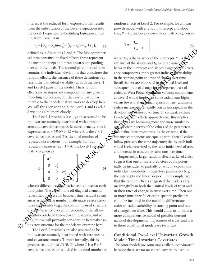
The Level-1 residuals (i.e., eti) are assumed to be multivariate normally distributed with a mean of zero and covariance matrix r; more formally, this is expressed as eti ∼ MVN (0, r) where r is the T × T covariance matrix and T is the total number of repeated observations. For example, for four repeated measures (i.e., T = 4) the Level-1 residual matrix is given as

R =

�

�

�

�

12

22

32

42

0

0 0

0 0 0

, (4)

where a different residual variance is allowed at each time-point. The zeros in the off-diagonal elements reflect that there are no between-time residual covari-ances estimated. A number of alternative error struc-tures are possible (e.g., the commonly used structure of equal variance over all time-points, or the allow-ance for correlated time-adjacent residuals, and so on), but we will primarily consider the heteroskedas-tic error structure for the models we examine here.

The Level-2 residuals are also assumed to be multivariate normally distributed with zero means and covariance matrix T; more formally, this is given as [u0i, u1i] ∼ MVN (0, T) where T is a P × P covariance matrix for which P is the total number of

random effects at Level 2. For example, for a linear growth model with a random intercept and slope (i.e., P = 2), the Level-2 covariance matrix is given as

T =

�

� �

00

10 11

,

(5)

where τ00 is the variance of the intercepts, τ11 is the variance of the slopes, and τ10 is the covariance between the intercepts and slopes. Larger Level-2 vari-ance components imply greater individual variability in the starting point and rate of change over time. Recall that we are interested in the initial level and subsequent rate of change in self-reported trust of cadets at West Point. Significant variance components at Level 2 would imply that some cadets start higher versus lower in their initial reports of trust, and some cadets increase more rapidly versus less rapidly in the development of trust over time. In contrast, as these Level-2 random effects approach zero, this implies that cadets are becoming more and more similar to one another in terms of the values of the parameters that define their trajectories. At the extreme, if the variance components are equal to zero, then all cadets follow precisely the same trajectory; that is, each indi-vidual is characterized by the same initial level of trust and increase in trust at the same rate over time.

Importantly, larger random effects at Level 2 also suggest that one or more predictors could poten-tially be included to partially or wholly explain the individual variability in trajectory parameters (e.g., the intercepts and linear slopes). For example, say that the random effects suggested that cadets vary meaningfully in both their initial levels of trust and in their rates of change in trust over time. Then one or more time-specific or cadet-specific predictors could be included in the model to differentiate cadet-to-cadet variability in starting point and rate of change over time. This would allow us to build a more comprehensive model of possible determi-nants of developmental trajectories of trust, and it is to these conditional models we turn next.

Conditional Two-Level Univariate Growth Model: Time-Invariant CovariatesThe prior models are sometimes called unconditional because there are no measured covariates used to

© 2012

AMERIC

AN PSYCHOLOGICAL A

SSOCIATIO

N. ALL RIG

HTS RESERVED

Curran et al.

338

predict the random parameters that define the growth trajectory.2 We can easily expand the uncon-ditional growth model to include one or more pre-dictors at either Level 1, Level 2, or both. Predictors that are characteristics of the individual and thus do not change as a function of time are called time-in-variant covariates (or TICs), and these are entered into the Level-2 equations. Examples of TICs might be biological sex, country of origin, ethnicity, or cer-tain genetic characteristics. In some applications, the TIC might in principle change over time, but for empirical or substantive reasons, only the initial assessment is considered (e.g., Curran, Stice & Chas-sin, 1997). Because TICs only enter at Level 2, the Level-1 equation remains as defined in Equation 1. However, the Level-2 equation is expanded to include one or more person-specific measures that are constant over time.

For example, assuming a linear growth model defined at Level 1, a single person-specific TIC, denoted wi, is included as

� � �

� � �

0 00 01 0

1 10 11 1

i i i

i i i

w r

w r

= + += + + ,

(6)

where β01 and β11 capture the expected shift in the conditional means of the intercept and slope compo-nents associated with a one-unit shift in the TIC. For example, positive coefficients would reflect that higher values on the TIC are associated with higher initial values and steeper rates of change over time. Importantly, these shifts in the conditional means are independent of the passage of time, highlighted by the fact that the TICs are not subscripted by t to represent time. Thus, one might find that the devel-opmental trajectories of trust in male cadets are defined by a different starting point and different rate of change relative to female cadets. These TICs could even be allowed to interact with one another— for example, the difference in trajectories of trust between male and female cadets could depend in part on the gender of the squad leader.

The inclusion of TICs is a powerful component of the MLM growth model. However, there may be important covariates we want to consider that are

not constant over time. Instead, one or more covari-ates might take on a unique value at any given time-point, and treating these as invariant over time would be inappropriate (Curran & Bauer, 2011). This type of predictor can be included within the MLM as a time-varying covariate.

Conditional Two-Level Univariate Growth Model: Time-varying CovariatesIn contrast to the TICs that are assumed to be con-stant over time, time-varying covariates (or TVCs) can take on a unique value at any given point in time. For example, covariates such as peer influence, anxiety, delinquency, or substance use would be expected to change from time-point to time-point, and it is critical that these temporal fluctuations be incorporated into the model (e.g., Curran & Bauer, 2011; Curran, Lee, MacCallum, & Lane, in press). Because the value of the TVC is unique to a given individual and a given time-point, these covariates enter directly into the Level-1 equations.

For example, the Level-1 model with a single TVC, denoted zti, is given as

y time z eti i i ti i ti ti= + + +� � �0 1 2 . (7)

Although π0i and π1i continue to represent the individual-specific intercept and slope components of the growth trajectory, these are now net the influ-ence of the TVC (and vice versa). In other words, these are the parameters of the trajectory of the out-come controlling for the effects of the TVC. The impact of the TVC on the outcome is captured in π2i which represents the shift in the mean of the out-come y at time t per one-unit shift in the TVC at the same time t. Importantly, whereas the TICs shift the conditional means of the trajectory parameters, the TVCs shift the conditional means of the outcome above and beyond the influence of the underlying growth trajectory. For example, the outcome of interest might be a cadet’s trust, and the TVC is a measure of perceived integrity in that same individ-ual; the TVC model would allow for the estimation of a developmental trajectory of trust, while simulta-neously including the time-specific influence of

2This is a bit of a misnomer given that time is a predictor at Level 1, yet the term unconditional commonly implies no predictors in addition to the mea-sure of time.

© 2012

AMERIC

AN PSYCHOLOGICAL A

SSOCIATIO

N. ALL RIG

HTS RESERVED

A Multivariate Growth Curve Model for Three-Level Data

339

perceived integrity. Allowing integrity to vary in value over time is a marked improvement over using just the initial measure of integrity as a TIC because much additional time-specific information is incor-porated into the model.

A particularly interesting aspect of the TVC model is that the magnitude of the effect of the TVC on the outcome can vary randomly across individu-als. The inclusion of this random effect is not required and would be determined on the basis of substantive theory or empirical necessity. This can most clearly be seen in the Level-2 equations that correspond to the TVC model defined in Equation 7:

� �

� �

� �

0 00 0

1 10 1

2 20 2

i i

i i

i i

r

r

r

= += += + ,

(8)

where β00, β10, and β20 represent the mean of each random term, and the corresponding residuals rep-resent the individually varying deviations around these means. Including the term r2i allows for the magnitude of the relation between the TVC and the outcome to vary randomly over individuals; omit-ting this term implies that the magnitude of the TVC effects is constant for all individuals. These level-2 equations could easily be expanded to include one or more TICs to examine predictors of each random Level-1 effect, but we do not explore this further here (for further details, see Raudenbush & Bryk, 2002; Singer & Willett, 2003).

The TVC model offers a powerful and flexible method for examining individual variability in change over time as a function of one or more pre-dictors that also vary as a function of time. One aspect of the TVC model that must be appreciated is that whereas an explicit growth process is estimated with respect to the outcome (i.e., yti), no such growth process is estimated with respect to the TVC (i.e., zti). In other words, although the TVC can take on unique values at any given time-point, it is not systematically related to the passage of time (e.g., Curran & Bauer, 2011). In many applications of the TVC model, this restriction is completely appropri-ate. One might be interested in examining trajecto-ries of reading ability having controlled for the time-specific effects of days of instruction missed

(Raudenbush & Bryk, 2002, p. 179) or in examining trajectories of heavy alcohol use having controlled for the time-specific effects of a new marriage (Cur-ran, Muthén, & Harford, 1998) or in a large variety of applications of daily diary studies (e.g., Bolger, Davis, & Rafaeli, 2003). In all of these examples, the TVC would not even be theoretically expected to change systematically over time. There are a variety of other examples in which the TVC is uniquely well suited to test the important questions of substantive interest.

Yet there are other situations in which substan-tive theory would not only predict that the TVC might take on different values over time, but that the TVC is itself developing systematically as a function of time. That is, the TVC may be expected to be characterized by a smoothed underlying trajectory that is defined by both fixed and random effects (Curran & Bauer, 2011). Our earlier hypothetical example considered the development of trust as the outcome and perceived integrity as the TVC. How-ever, this strongly assumes that integrity is not devel-oping systematically over time. Yet theory predicts that both trust and integrity codevelop systematically over time, and arbitrarily treating one of these con-structs as a criterion and the other as a TVC would not correspond to our substantive theory. Further-more, the core theoretical question of interest may not be related to how the time-specific value of the TVC is related to the time-specific value of the out-come (as is tested in the TVC model); instead, it may be how the parameters of the trajectory of the TVC relate to the parameters of the trajectory of the out-come. This is sometimes described as examining how two or more constructs “travel together” through time (e.g., McArdle, 1989). To test ques-tions such as these, we must move to a multivariate growth model that allows for the simultaneous esti-mation of growth in both the outcome and the TVC.

Two-Level Multivariate Growth ModelOur goal is to define a model that allows for the esti-mation of growth processes in two or more con-structs simultaneously. This is a distinct challenge given that the standard multilevel model is inher-ently univariate in that it is limited to a single crite-rion measure (e.g., Raudenbush & Bryk, 2002,

© 2012

AMERIC

AN PSYCHOLOGICAL A

SSOCIATIO

N. ALL RIG

HTS RESERVED

Curran et al.

340

Equation 14.1). These univariate models have been expanded to the multivariate setting by Goldstein (1995), Goldstein et al. (1993), and MacCallum et al. (1997), among others; we draw on this collected body of work here.

The key to approaching this problem is to stack our multiple criterion variables into a newly created variable that is nominally univariate (i.e., there is just one variable), but this variable actually contains repeated assessments on two or more outcomes over time. This is sometimes called a synthesized variable (e.g., MacCallum et al., 1997). We will then incor-porate a series of dummy variables as exogenous predictors that will give us full control of which spe-cific outcomes we are referencing within different parts of the model. This will ultimately allow us to use our standard univariate multilevel modeling framework to fit what is in actuality a rather com-plex multivariate structure.

We begin by defining a simple linear growth model at Level 1, but we will add superscripts to all of the terms to identify to which outcome the term is associated. We use a linear trajectory here, but a variety of alternative functional forms could be used instead. Furthermore, a different form of growth could be used for each of the individual outcomes (e.g., linear in one outcome and quadratic in another). The general expression for k = 1, 2, . . . , K multivariate outcomes is

y time eti

k

i

k

i

k

ti

k

ti

k( ) ( ) ( ) ( ) ( )= + +� �0 1 . (9)

So yti

1( ) would represent the outcome for the first construct (where k = 1; e.g., trust) and yti

2( ) would represent the outcome for the second construct (where k = 2; e.g., integrity), and so on. The level-2 equations are also modified to denote whether the term is associated with the first criterion measure (k = 1) or the second (k = 2):

� �

� �

0 00 0

1 10 1

i

k k

i

k

i

k k

i

k

r

r

( ) ( ) ( )

( ) ( ) ( )= +

= + . (10)

Compare this with Equation 2 to see the direct parallel between the Level-2 univariate and multi-variate expressions. Finally, the reduced form expression is given as

y time r r titi

k k k

ti

k

i

k

i

k( ) ( ) ( ) ( ) ( ) ( )= +( ) + +� �00 10 0 1 mme eti

k

ti

k( ) ( )+( ). (11)

We can combine these equations into a single multivariate expression in which there is a single synthesized criterion variable that we arbitrarily denote dvti to represent the dependent variable dv at time t for individual i. In other words, we manu-ally create a new variable in the data set that stacks the multiple outcome variables into a single- column vector. Because multiple outcomes are now contained in a single variable, we must include additional information to distinguish which specific element belongs to which specific outcome. To do this, we create two or more new variables (denoted δk) that are simple binary dummy variables that represent which specific out-come is under consideration. There are K dummy variables, one each for k = 1,2, . . . K outcomes. The dummy variable is δk = 1 for construct k, and is equal to zero otherwise. (We will show a specific example of this in a moment.)

Finally, we can fit a single model to this new data structure in which a separate growth process is simultaneously fitted to each outcome k, the specific outcome of which is toggled in or out of the equa-tion using an overall summation weighted by the dummy variables (e.g., MacCallum et al., 1997). More specifically, the general expression for the reduced-form model is

dv time

r r

ti k

k k

ti

k

k

K

i

k

= +( )

+ +

( ) ( ) ( )

=

( )

∑� � �00 101

0 11i

k

ti

k

ti

ktime e( ) ( ) ( )+( ). (12)

In words, Equation 12 defines the growth trajectory for each outcome of interest, and the dummy codes include or exclude the relevant values in the synthe-sized dependent variable through the overall summation.

To further explicate this, we can consider just the bivariate case in which K = 2. We define k = 1 to represent yti and k = 2 to represent zti, and we super-script with y and z to identify to which outcome each term belongs. For example, y might represent trust and z might represent integrity. In this case, Equation 12 simplifies to

dv time r r titi y

y y

ti

y

i

y

i

y= +( ) + +( ) ( ) ( ) ( ) ( )� � �00 10 0 1 mme e

time

ti

y

ti

y

z

z z

ti

z

( ) ( )

( ) ( ) ( )

+( )

+ +(� � �00 10 )) + + +( )

( ) ( ) ( ) ( )r r time ei

z

i

z

ti

z

ti

z

0 1 .

(13)

© 2012

AMERIC

AN PSYCHOLOGICAL A

SSOCIATIO

N. ALL RIG

HTS RESERVED

A Multivariate Growth Curve Model for Three-Level Data

341

This expression highlights that this requires an atyp-ical definition of the model relative to the standard two-level TVC growth model. To see this, we will first distribute the two binary variables and gather up our terms:

dv time

r r

ti

y

y

y

y ti

y

i

y

y i

= +( )+ +

( ) ( ) ( )

( )

� � � �

�

00 10

0 1

yy

y ti

y

ti

y

y

z

z

z

z

time e

ti

( ) ( ) ( )

( ) ( )

+( )+ +

� �

� � � �00 10 mme

r r time e

ti

z

i

z

z i

z

z ti

z

ti

z

z

( )

( ) ( ) ( ) ( )

( )+ + +0 1� � �(( ). (14)

There are two somewhat-odd things about this expression relative to the usual univariate growth model. First, there is no overall intercept term for this reduced-form model. Instead, the intercept for the first outcome (i.e., yti) is captured in the main effect of the first dummy variable (i.e., � �00

y

y( ) ); simi-

larly, the intercept for the second outcome (i.e., zti) is captured in the main effect of the second dummy variable (i.e., � �00

z

z( ) ). Second, the linear slope for

each outcome is captured in the interaction between each dummy variable and time. Specifically, the lin-ear slope for the first outcome (i.e., yti) is captured in the interaction of the first dummy variable and time (i.e., � �10

y

y ti

ytime( ) ( )); the linear slope for the second outcome (i.e., zti) is captured in the interac-tion of the second dummy variable and time (i.e., � �10

z

z ti

ztime( ) ( )). Thus, the main effects of the dummy variables represent the outcome-specific intercepts, and the interactions between the dummy variables and time represent the outcome-specific slopes. See MacCallum et al. (1997) for an excellent description and demonstration of this model with three outcomes.

There are a number of advantages to this model expression, a key one of which is the inclusion of more complex error structures at both level 1 and level 2 than is possible within the univariate TVC growth model. The reason is that the covariance structure not only holds within each construct sepa-rately (e.g., within yti and within zti), but it also holds across construct. For example, a univariate growth model of trust examines covariance struc-tures only within trust; and a univariate growth model of integrity examines covariance structures only within integrity. But a multivariate growth

model of trust and integrity allows for the examina-tion of covariance structures between trust and integ-rity both at the time-specific (i.e., Level-1) and trajectory-specific (i.e., Level-2) parts of the model. This can be critically important information to include, not only in terms of properly modeling the joint structure of the observed data but also in terms of fully evaluating the substantive research question of interest.

For example, consider the Level-1 covariance structure for the bivariate model of yti and zti (i.e., the model defined in Equation 14). The corresponding Level-1 covariance structure is e e e e e e ei

y

i

y

i

y

i

y

i

z

i

z

i

z

1 2 3 4 1 2 3( ) ( ) ( ) ( ) ( ) ( ) (, , , , , , )) ( ) ( ), ~ ,e MVNi

z

4 0 R with matrix elements

R =

( )

( )

( )

( )

( )

�

�

�

�

� �

1

2

2

2

3

2

4

2

11 1

2

0

0 0

0 0 0

0 0 0

y

y

y

y

z y z, (( )

( ) ( )

( ) ( )0 0 0 0

0 0 0 0 0

0 0 0

22 2

2

33 3

2

44

� �

� �

�

z y z

z y z

z

,

,

,,y z( ) ( )

0 0 0 4

2�

.

(15)

The upper left quadrant represents the Level-1 residual covariance structure among the four repeated assessments of yti; this is equivalent to those of the univariate model shown in Equation 4. Similarly, the lower-right quadrant represents the Level-1 residual covariance structure among the four repeated assessments of zti. However, critically important information is contained in the lower left quadrant in the form of the within-time but across-construct residual covariance structure. For exam-ple, the element �11

z y,( ) represents the covariance between the Level-1 residuals of yti and zti at the first time-point (i.e., t = 1). This captures the part of trust at Time 1 that is unexplained by the trajectory of trust that covaries with the part of integrity at Time 1 that is unexplained by the trajectory of integrity. This provides a way to include potentially important covariances among the time-specific Level-1 residu-als across the two or more multivariate outcomes, the omission of which could artificially inflate the variance components at Level 2.

The multivariate model also allows us to examine across-construct covariances among the Level-2

© 2012

AMERIC

AN PSYCHOLOGICAL A

SSOCIATIO

N. ALL RIG

HTS RESERVED

Curran et al.

342

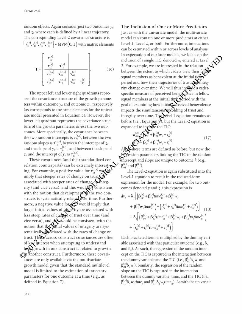
random effects. Again consider just two outcomes yti and zti where each is defined by a linear trajectory. The corresponding Level-2 covariance structure is

r r r r MVNi

y

i

y

i

z

i

z

0 1 0 1 0( ) ( ) ( ) ( ) ( ), , , ~ ,T with matrix elements

T =

( )

( ) ( )

( ) ( ) ( )

�

� �

� � �

�

00

10 11

00 01 00

10

y

y y

z y z y z

z

, ,

,yy z y z z( ) ( ) ( ) ( )

� � �11 10 11

,

. (16)

The upper left and lower right quadrants repre-sent the covariance structure of the growth parame-ters within outcome yti and outcome zti, respectively (as corresponds to the same elements for the univar-iate model presented in Equation 5). However, the lower left quadrant represents the covariance struc-ture of the growth parameters across the two out-comes. More specifically, the covariance between the two random intercepts is �00

z y,( ), between the two random slopes is �11

z y,( ), between the intercept of zti and the slope of yti is �01

z y,( ), and between the slope of zti and the intercept of yti is �10

z y,( ).These covariances (and their standardized cor-

relation counterparts) can be extremely interest-ing. For example, a positive value for �11

z y,( ) would imply that steeper rates of change on trust are associated with steeper rates of change on integ-rity (and vice versa), and this would be consistent with the notion that development in the two con-structs is systematically related over time. Further-more, a negative value for �01

z y,( ) would imply that larger initial values of integrity are associated with less steep rates of change of trust over time (and vice versa), and this would be consistent with the notion that the initial values of integrity are sys-tematically associated with the rates of change on trust. These across-construct covariances are often of key interest when attempting to understand how growth in one construct is related to growth in another construct. Furthermore, these covari-ances are only available via the multivariate growth model given that the standard multilevel model is limited to the estimation of trajectory parameters for one outcome at a time (e.g., as defined in Equation 7).

The Inclusion of one or More PredictorsJust as with the univariate model, the multivariate model can contain one or more predictors at either Level 1, Level 2, or both. Furthermore, interactions can be estimated within or across levels of analysis. In expectation of our later models, we focus on the inclusion of a single TIC, denoted wi, entered at Level 2. For example, we are interested in the relation between the extent to which cadets view their fellow squad members as benevolent at the initial time period and how their trajectories of trust and integ-rity change over time. We will thus include a cadet-specific measure of perceived benevolence in fellow squad members at the initial time period with the goal of examining how initial perceived benevolence impacts the simultaneous unfolding of trust and integrity over time. The Level-1 equation remains as before (i.e., Equation 9), but the Level-2 equation is expanded to include the TIC:

� � �

� � �

0 00 01 0

1 10 11

i

k k k

i i

k

i

k k k

w r( ) ( ) ( ) ( )

( ) ( )= + +

= + (( ) ( )+w ri i

k

1 . (17)

All of these terms are defined as before, but now the regression parameters linking the TIC to the random intercept and slope are unique to outcome k (e.g., �01

k( ) and �11

k( )).The Level-2 equation is again substituted into the

Level-1 equation to result in the reduced-form expression for the model. For example, for two out-comes denoted y and z, this expression is

dv time wti y

y y

ti

y y

i= + +(+

( ) ( ) ( ) ( )� � � �

�

00 10 01

11

yy

i ti

y

i

y

i

y

ti

y

ti

yw time r r time e( ) ( ) ( ) ( ) ( ) ( ))+ + +( 0 1 ))

+ + + +( ) ( ) ( ) ( ) ( )� � � � �z

z z

ti

z z

i

ztime w00 10 01 11 ww time

r r time e

i ti

z

i

z

i

z

ti

z

ti

z

( )

( ) ( ) ( ) (

( )

+ + +0 1))( ).

(18)

Each bracketed term is multiplied by the dummy vari-able associated with that particular outcome (e.g., δy and δz). As such, the regression of the random inter-cept on the TIC is captured in the interaction between the dummy variable and the TIC (i.e., � �01

y

y iw( ) and � �01

z

z iw( ) ). Similarly, the regression of the random slope on the TIC is captured in the interaction between the dummy variable, time, and the TIC (i.e., � �11

y

y i tiw time( ) and � �11

z

z i tiw time( ) ). As with the univariate

© 2012

AMERIC

AN PSYCHOLOGICAL A

SSOCIATIO

N. ALL RIG

HTS RESERVED

A Multivariate Growth Curve Model for Three-Level Data

343

two-level model, the TIC shifts the conditional means of the random intercepts and slopes per unit shift in the TIC. In the multivariate model, however, these mean shifts affect all outcomes simultaneously.

Now that we have laid out the model equations, we find that a key practical challenge in fitting these models to real data is the need to restructure the data in a way that is not necessarily intuitive but that is needed to allow for proper model estimation. Despite the nonintuitiveness, a bit of careful thought shows that this can be accomplished in a straightforward manner; we demonstrate this in the next section.

data structure for the Two-Level Multivariate Growth ModelAn example of the data structure for the standard organization for the univariate TVC model is

presented in the left panel of Figure 17.1. A sample data structure is given for four individuals where col-umn i denotes the identification number of each per-son, column t denotes time-point, column yti denotes the criterion (e.g., trust), column zti denotes the TVC (e.g., integrity), and column wi denotes a Level-2 TIC (e.g., benevolence). This is precisely how the data would be structured in the standard univariate growth model with one TVC and one TIC.

Compare this standard structure to that pre-sented in the right panel of Figure 17.1 that is refor-matted for the bivariate model. Note that these are precisely the same data as are shown in the left panel except for two key differences. First, the values on yti and zti are now strung out in a single column labeled dvti; this represents the newly synthesized criterion variable that we manually created and will be the

i t yti zti wi i t dvti wi δy δz

1 1 y11 z11 w1 1 1 y11 w1 1 01 2 y21 z21 w1 1 1 z11 w1 0 11 3 y31 z31 w1 1 2 y21 w1 1 01 4 y41 z41 w1 1 2 z21 w1 0 12 1 y12 z12 w2 1 3 y31 w1 1 02 2 y22 z22 w2 1 3 z31 w1 0 12 3 y32 z32 w2 1 4 y41 w1 1 02 4 y42 z42 w2 1 4 z41 w1 0 13 1 y13 z13 w3 2 1 y12 w2 1 03 2 y23 z23 w3 2 1 z12 w2 0 13 3 y33 z33 w3 2 2 y22 w2 1 03 4 y43 z43 w3 2 2 z22 w2 0 14 1 y14 z14 w4 2 3 y32 w2 1 04 2 y24 z24 w4 2 3 z32 w2 0 14 3 y34 z34 w4 2 4 y42 w2 1 04 4 y44 z44 w4 2 4 z42 w2 0 1

3 1 y13 w3 1 03 1 z13 w3 0 13 2 y23 w3 1 03 2 z23 w3 0 13 3 y33 w3 1 03 3 z33 w3 0 13 4 y43 w3 1 03 4 z43 w3 0 14 1 y14 w4 1 04 1 z14 w4 0 14 2 y24 w4 1 04 2 z24 w4 0 14 3 y34 w4 1 04 3 z34 w4 0 14 4 y44 w4 1 04 4 z44 w4 0 1

FIGUre 17.1. standard data structure for a four-time-point two-level univariate growth model with one time-varying covariate (left panel) and the modified data structure for a four-time-point two-level bivariate growth model (right panel).

© 2012

AMERIC

AN PSYCHOLOGICAL A

SSOCIATIO

N. ALL RIG

HTS RESERVED

Curran et al.

344

unit of analysis for the multivariate model. Second, the TIC remains constant across individuals but is now repeated for each outcome. Third, there are two new dummy variables, denoted δy and δz, each of which is equal to one when the corresponding ele-ment in dvti is from that construct, and zero other-wise. For example, in the first row of data δy = 1 and δz = 0 because the element of dvti is from outcome yti; similarly, in the second row of data δy = 0 and δz = 1 because the element of dvti is from outcome zti. This pattern repeats throughout the entire data matrix. The multivariate growth model can now be fitted directly to these newly structured data.3

Three-LeveL GrowTh ModeLs

All of the models that we have explored thus far assume that the data structure is nested. That is, repeated measures are nested within individual, and this necessitates the two-level model. Importantly, this structure in turn implies that the individual subjects in the sample are mutually independent. In other words, it is strongly assumed that no two indi-viduals are any more or less similar than any other two. This assumption is commonly met in practice, especially when subjects are obtained using some form of simple random sampling procedure, and subjects are not themselves nested in some higher structure (e.g., Raudenbush & Bryk, 2002).

However, there are many situations in which not only are the repeated measures nested within indi-viduals but also individuals are in turn nested within groups. A common example is when repeated mea-sures are nested within children, and children are in turn nested within classroom. In our case, we have repeated measures nested within cadet, and cadets are in turn nested within squads. Such a data struc-ture would violate the assumptions of the two-level model because two cadets who are members of the same squad are likely to be more similar to one another than two cadets from different squads. A major strength of the multilevel model is the natural way that it may be expanded to many complex sam-pling designs, including three levels of nesting. But these models are understandably more complex, and

we must closely consider how the necessary expan-sions are possible in the multivariate case.

Three-Level Unconditional Univariate Growth ModelWe will begin by moving back to the two-level uni-variate model and then extending it to allow for three levels of nesting. Our motivating example is time nested within cadet, and cadet is nested within squad. The Level-1 model becomes

y time etij ij ij tij tij= + +� �0 1 , (19)

where t and i continue to represent time and individ-ual, respectively, but now j denotes group member-ship at level 3 (j = 1, 2, . . . , J). More specifically, ytij is the obtained measure on outcome y at time t for individual i nested in group j; π0ij and π1ij are the intercept and slope for individual i in group j; timetij is the numerical measure of time at time t for indi-vidual i in group j, and etij is the time-, individual-, and group-specific residual where etij ∼ MVN (0, r).

The Level-2 equations are

� �

� �

0 00 0

1 10 1

ij j ij

ij j ij

r

r

= +

= + , (20)

where β00j and β10j are the group-specific intercept and slope of the linear trajectory. These terms are sometimes a bit tricky to think about at first. The group-specific intercept and slope (i.e., β00j and β10j) represent the mean of the intercepts and the mean of the slopes of the growth trajectories for all of the individuals nested within group j. For example, these might represent the mean initial value and mean rate of change in trust for all of the cadets who are nested within a given squad j. As such, the residuals r0ij and r1ij represent the deviation of each individual’s inter-cept and slope around their group-specific mean val-ues. That is, the residuals capture the variability of each cadet’s trajectory of trust around their own squad-specific means trajectory of trust. More for-mally, this is given as [r0ij, r1ij] ∼ MVN (0, Tπ); we will explore the Tπ covariance matrix of random effects more closely in a moment.

3A detailed example of this restructuring is available from Patrick J. Curran or from http://www.unc.edu/∼curran

© 2012

AMERIC

AN PSYCHOLOGICAL A

SSOCIATIO

N. ALL RIG

HTS RESERVED

A Multivariate Growth Curve Model for Three-Level Data

345

Finally, given the three-level structure of the data, the group-specific intercepts and slopes (e.g., β00j and β10j) themselves vary randomly across groups. The Level-3 equations are thus

� �

� �

00 000 00

10 100 10

j j

j j

u

u

= +

= + , (21)

where γ000 and γ100 represent the grand mean inter-cept and slope pooling over all individuals and all groups, and the residual terms u00j and u10j capture the deviation of each group-specific value from the grand means, and [u00j, u10j] ∼ MVN (0, Tβ). The reduced form expression for the three-level univari-ate growth model is

y time

u r u time

tij tij

j ij j tij

= +( )+ + + +

� �000 100

00 0 10 rr time eij tij tij1 +( ). (22)

See Raudenbush and Bryk (2002, Chapter 8) for an excellent description of the general three-level model as well as a discussion of studying individual change within groups.

A key characteristic of this model is the estimation of random components at both levels two and three, and the covariance structures of these random effects will be of specific interest in the models described in the section Three-Level Multivariate Growth Model. In the two-level model, the Level-2 covariance matrix was denoted T. In the three-level model, however, there is a T matrix at Level 2 and at Level 3. This is why we must distinguish these T matrixes with the use of an additional subscript: Tπ for Level 2 and Tβ for Level 3. Let us first consider the covariance struc-ture of the residuals at Level 2 captured in Tπ.

For a linear model defined at Level 1, the Level-2 covariance matrix takes the form

T�

�

� �

�

� �=

00

01 11

, (23)

where τπ00 represents the Level-2 variance of the intercepts, τπ11 the variance of the slopes, and τπ01 the covariance between the intercepts and slopes. These are sometimes challenging estimates to inter-pret given that they reside at the middle level of nesting. Specifically, these estimates represent the amount of variability among the individual-specific

trajectories within group (e.g., variability among tra-jectories of trust for each cadet sharing the same squad). Thus, larger values reflect greater person-to-person variability in the trajectories within group; similarly, smaller values reflect greater person-to-person similarity in the trajectories within group. At the extreme, if these variance components equal zero, then each person within the group is charac-terized by the same trajectory. For example, a larger value of τπ11 would imply greater variability in rates of change in trust among cadets within the same squad. If τπ11 = 0 then every cadet within each squad is characterized by precisely the same developmen-tal trajectory of trust over time. Although this implies that there is no cadet-to-cadet variability in the development of trust within squad, this does not imply that there is no meaningful squad-to-squad variability in the development of trust over time. To assess this, we must turn to the Level-3 covariance matrix of random effects.

The covariance matrix of random effects at the third level of analysis is denoted Tβ. For the linear model with full random effects defined in Equation 22), the elements of this matrix are

T�

�

� �

�

� �=

00

01 11

, (24)

where τβ00 represents the Level-3 variance of the intercepts, τβ11 the variance of the slopes, and τβ01 the covariance between the intercepts and slopes. In contrast to the Level-2 variance components that capture individual-level variability of the trajectory parameters within group (e.g., squad), Tβ captures the group-to-group level variability of the trajectory parameters between group. For example, larger val-ues of τβ00 and τβ11 would indicate greater squad-to-squad variability in intercepts and slopes; that is, some squads are characterized by higher versus lower starting points on the outcome variables and larger versus smaller rates of change over time. Alternatively, smaller values indicate less variability in the trajectory parameters across squad. For exam-ple, larger variance components would imply that there are potentially meaningful differences in the squad-level trajectories of trust over time across the set of squads; some squads might be defined by

© 2012

AMERIC

AN PSYCHOLOGICAL A

SSOCIATIO

N. ALL RIG

HTS RESERVED

Curran et al.

346

higher starting points and steeper rates of change, whereas others are not. At the extreme, values of zero reflect that all squads are governed by the same trajectory parameters; for example, all squads are defined by the same starting point of trust and same rate of change in trust over time. Indeed, in this extreme case, the three-level model simplifies to the two-level structure defined earlier given that there is no meaningful squad-to-squad variability.

To briefly summarize, the Level-1 variance compo-nents reflect the time-specific variations in trust around each cadet’s trajectory of trust; the Level-2 vari-ance components reflect the cadet-specific variations in the trajectories of trust around the mean trajectory of trust within each squad; and the Level-3 variance com-ponents reflect the squad-specific variations in the tra-jectories of trust around the grand mean trajectory of trust pooling over all cadets and all squads. This break-down of the random effects is one of the most elegant aspects of the three-level model: The total variability observed in trust can be broken down into time- specific, cadet-specific, and squad-specific effects. And if meaningful random effects are identified at any level of analysis, one or more predictors can be included to attempt to explain these variations.

Three-Level Conditional Univariate Growth ModelJust as with the two-level model, covariates can be included at any level of analysis. In the three-level model, however, predictors can be time specific (i.e., Level-1 model), person specific (i.e., Level-2 model), or group specific (i.e., Level-3 model). Using our previous terminology, TVCs would thus appear at Level 1, and individual- and group-specific TICs would appear at Levels 2 and 3, respectively. Given our primary interest in change in two or more constructs over time, here we will focus just on the TVCs at Level 1; inclusion of TICs is a natural extension of the two-level model described earlier (e.g., Raudenbush & Bryk, 2002, pp. 241–245).

The Level-1 equation for a simple linear growth model with one TVC is defined as

y time z etij ij ij tij ij tij tij= + + +� � �0 1 2 , (25)

where ztij is the time-, person-, and group-specific TVC, and π2ij captures the relation between the TVC

and the outcome at time-point t. The magnitude of the relation between the TVC and the outcome can vary randomly over individual with corresponding Level-2 equations

� �

� �

� �

0 00 0

1 10 1

2 20 2

ij j ij

ij j ij

ij j ij

r

r

r

= +

= +

= + ,

(26)

where β20j represents the mean relation between the TVC and the outcome pooling over all individuals within group j. Finally, the magnitude of these within-group specific effects can itself vary over group, and this is captured in the Level-3 equations

� �

� �

� �

00 000 00

10 100 10

20 200 20

j j

j j

j j

u

u

u

= +

= +

= + .

(27)

The reduced form results from the substitution of Equation 27 into 26, and Equation 26 subse-quently into Equation 25. Although tedious, it is interesting to see the full set of collected terms:

y time z u r

tim

tij tij tij j ij= + +( ) + +( )� � �000 100 200 10 0

ee u r z u r etij ij tij tij j ij tij+ +( ) + + +( )2 00 0 . (28)

This model is in the same form as its two-level counterpart with the key exception that an additional covariance matrix is allowed to capture between-group variability at the third level of nesting. We again assume, however, that although the TVC can take on a different numerical value at each time-point t, the TVC itself is assumed to not change systemati-cally over time. Whether by theoretical rationale or empirical necessity, there are many situations in which we would like to expand the univariate three-level model to simultaneously capture growth in two or more constructs over time. Whereas the two-level multivariate model is well established in the literature (e.g., MacCallum et al., 1997), we are unaware of any prior presentation of the expansion of this model to three levels of nesting. It is to this that we now turn.

Three-Level Multivariate Growth ModelThe expansion of the multivariate growth model from two to three levels of nesting is both intuitive

© 2012

AMERIC

AN PSYCHOLOGICAL A

SSOCIATIO

N. ALL RIG

HTS RESERVED

A Multivariate Growth Curve Model for Three-Level Data

347

and straightforward. Just as we expanded the uni-variate growth model to allow for individuals to be nested within group, we will expand the multivari-ate model in precisely the same way. Indeed, we will use the same dummy variable approach to combine the multiple outcomes into a single three-level model. The only difference here is that the reduced form expression is more complex because of the nesting of time within individual within group.

The general expression is

dv time utij k

k k

tij

k

k

K

j= +( ) +( ) ( ) ( )

=∑� � �000 100

100

kk

ij

k

j

k

tij

k

ij

k

tij

r

u time r time

( ) ( )

( ) ( ) ( )

+(+ +

0

10 1

kk

tij

ke( ) ( )+ ) (29)

for k = 1, 2, . . . , K outcomes. There is no need to modify the notation for the dummy variables to include information about group membership because the dummy variables only demarcate to which outcome variable the numerical value belongs; this is not unique to time, person, or group. For the bivariate case, this simplifies to

dv time u rtij y

y y

tij

y

j

y

i= +( )+ +( ) ( ) ( ) ( )� � �000 100 00 0 jj

y

j

y

tij

y

ij

y

tij

yu time r time e

( )

( ) ( ) ( ) ( )

(

+ + +10 1 ttij

y

z

z z

tij

ztime u

( )

( ) ( ) ( )

)+ +( )

+� � �000 100 000 0

10 1

j

z

ij

z

j

z

tij

z

ij

z

ti

r

u time r time

( ) ( )

( ) ( ) ( )

+(+ + jj

z

tij

ze( ) ( )+ ),

(30)

where the first bracketed term captures the three-level growth process for outcome ytij (e.g., trust) and the second bracketed term captures the three-level growth process for outcome ztij (e.g., integrity). As before, these two growth processes need not be the same (e.g., the first could be linear and the second quadratic, and so on). As with the two-level multivar-iate expression, the definition of the model is atypical relative to the standard three-level growth model. The main effects of the two dummy codes are again the intercept of each construct, respectively, and the interaction between each dummy code and time are again the slope of each construct, respectively.

The key benefit stemming from this rather com-plex (yet intuitively appealing) model is the ability to explicitly incorporate various covariance struc-tures among the residual terms at all three levels

both within and across constructs. The Level-1 covariance structure for this model is the same as that defined in Equation 15 for the two-level model. However, the covariance structures at Levels 2 and 3 can become quite interesting. Given space con-straints and the similarity in the types of inferences that can be drawn, here we will focus primarily on the level-2 covariance structure as estimated both within and across the multivariate outcomes (i.e., Tπ). However, all of our descriptions would generalize naturally to the Level-3 covariance struc-ture (i.e., Tβ). Furthermore, these generalizations offer unique insights into the relations among growth trajectories at the level of the group. Thus Tπ estimates the random components of individual-level trajectories nested within groups, and Tβ esti-mates the random components of group-level trajectories across groups. Only the three-level model provides this joint estimation of within- and between-group effects (the specific parameterization of which would depend on substantive theory and empirical necessity).

To remain concrete, we will continue to consider the three-level bivariate growth model defined in Equation 30. There is thus a linear trajectory esti-mated for both outcomes, and all trajectory parame-ters are allowed to vary both at Level 2 and Level 3. The joint covariance structure for the two growth processes at Level 2 is contained in the matrix Tπ. The specific elements of this matrix are

T�

�

� �

� � �

�

� �

� � �=

( )

( ) ( )

( ) ( )

00

10 11

00 01 00

y

y y

z y z y, , zz

z y z y z z

( )

( ) ( ) ( ) ( )

� � � �

� � � �10 11 10 11

, ,

. (31)

Note the substantial similarity to the Level-2 covariance matrix from the two-level bivariate growth model defined in Equation 16. The critical difference between the Level-2 covariance matrix T from the two-level model and the Level-2 covariance matrix Tπ from the three-level model is that the lat-ter explicitly accounts for the clustering of individu-als within groups at the highest level of nesting. If we were to fix the Level-3 covariance matrix to zero

© 2012

AMERIC

AN PSYCHOLOGICAL A

SSOCIATIO

N. ALL RIG

HTS RESERVED

Curran et al.

348

(e.g., Tβ = 0), then the three-level model would reduce to the two-level model and the Level-2 cova-riance matrices defined in Equations 16 and 31 would be equal (e.g., T = Tπ).

The same pattern as was observed in the T matrix defined in Equation 16 holds here. Namely, the upper left and lower right quadrants represent the variance components of the trajectory parame-ters of the individuals nested within each group for outcome y and outcome z, respectively. Further-more, the lower left quadrant represents the vari-ance components across the two outcomes. For example, the element �

�00

z y,( ) captures the covariance between the random intercepts on outcome z with the random intercepts on outcome y; this element assesses the extent of similarity in the starting points of the trajectories of z and y of individuals nested within group. Similarly, the element �

�11

z y,( ) captures the covariance between the random slopes on out-come z with the random slopes on outcome y; this assesses the extent of similarity in the rates of change of the trajectories of z and y. Finally, the ele-ment �

�10

z y,( ) captures the covariance between the ran-dom slopes on z and the random intercepts on y, and �

�01

z y,( ) the covariance between the random inter-cepts on z with the random slopes on y. As with the two-level models, these covariances can be standard-ized into correlations for interpretation and effect size estimation.

These covariance estimates are often of key sub-stantive interest when testing hypotheses regarding stability and change over time. As in the two-level bivariate growth model, the lower-left quadrant of the Tπ matrix captures the similarity or dissimilarity in patterns of growth in the two outcomes over time. This can provide insight into a variety of interesting questions. For example, to what extent are the start-ing points of the trajectories of trust and integrity related? Is the rate of change in trust systematically related to the rate of change in integrity? Do individ-uals who report higher initial levels of trust also report steeper rates of change in integrity (and vice versa)? The key advantage of the three-level model is that these relations are estimated while properly allowing for the nesting of individuals within groups. Furthermore, similarly intriguing insights can be gained about group-level characteristics of

growth through the Level-3 variance components (i.e., Tβ) that would not otherwise be accessible via the two-level model. For example, on average, do squads that are characterized by higher initial levels of trust tend to increase more steeply in integrity over time? These are just a few of the many advan-tages of the multivariate–multilevel growth models.

The Inclusion of one or More PredictorsOne or more predictors can be included at any of the three levels of analyses. Furthermore, interac-tions can be estimated within one level, across two levels, or even across all three levels. Because the equations are direct extensions of those already defined, we do not repeat these here. For example, the inclusion of a single TIC at Level 2 follows the same structure as was defined in Equation 18 but with the addition of the necessary Level-3 error terms (for full details, see Raudenbush & Bryk, 2002, Chapter 8).

data structure for the Three-Level Multivariate Growth ModelThe data structure required to fit the three-level bivariate growth model is a direct extension of that used for the two-level model. For example, the left panel in Figure 17.2 presents the standard data struc-ture used to fit the three-level TVC model defined in Equation 22 to four individuals with the inclusion of a Level-2 TIC. There is more information here than was required for the two-level model given the need to simultaneously track group membership. Thus, column j denotes group, column i denotes individual, and column t denotes time. Subjects 1 and 2 are members of Group 1, and Subjects 3 and 4 are mem-bers of Group 2. Finally, ytij is the observed outcome variable, ztij is the TVC, and wij is the person-specific TIC. To combine the outcome and the TVC into a bivariate model, these must be restructured under a single column as the newly constructed (or synthe-sized) dependent variable.

These restructured data are shown in the right panel of Figure 17.2. Columns j, i, and t all remain as before, but there is a newly created column labeled dvtij; this is the newly synthesized variable that is a stacked vector of ytij and ztij. The TIC wij is again repeated over both the outcome variables.

© 2012

AMERIC

AN PSYCHOLOGICAL A

SSOCIATIO

N. ALL RIG

HTS RESERVED

A Multivariate Growth Curve Model for Three-Level Data

349

Finally, the binary variables denoted δy and δz again identify to which construct each element of the syn-thesized variable belongs. Note the significant simi-larities between the data structures presented in Figure 17.1 and Figure 17.2. The only meaningful difference is that Figure 17.1 implies that the four individuals are independent, whereas Figure 17.2 explicitly captures information about the group to which each individual belongs.4

We have now fully explicated the multivariate growth model for three levels of nesting, and we have described the data structure needed for estima-tion. We now turn to the application of these mod-els to evaluate several research hypotheses about the

development of trust and integrity over time using real empirical data drawn from a longitudinal study of military cadets.

eMPIrICaL exaMPLe: The LonGITUdInaL deveLoPMenT oF TrUsT In MILITary CadeTs

The core constructs of trust, influence, and leader-ship have long been a critically important focus of past and ongoing military research. Despite the wealth of knowledge that has been gathered, little is known about how trust and influence codevelop over time (e.g., Sweeney, 2007; Sweeney, Dirks,

4Examples of how to reorder univariate data to a multivariate structure are available from Patrick J. Curran or from http://www.unc.edu/∼curran

j i t ytij ztij wij j i t dvtij wij δy δz

1 1 1 y111 z111 w11 1 1 1 y111 w11 1 01 1 2 y211 z211 w11 1 1 1 z111 w11 0 11 1 3 y311 z311 w11 1 1 2 y211 w11 1 01 1 4 y411 z411 w11 1 1 2 z211 w11 0 11 2 1 y121 z121 w21 1 1 3 y311 w11 1 01 2 2 y221 z221 w21 1 1 3 z311 w11 0 11 2 3 y321 z321 w21 1 1 4 y411 w11 1 01 2 4 y421 z421 w21 1 1 4 z411 w11 0 12 3 1 y132 z132 w32 1 2 1 y121 w21 1 02 3 2 y232 z232 w32 1 2 1 z121 w21 0 12 3 3 y332 z332 w32 1 2 2 y221 w21 1 02 3 4 y432 z432 w32 1 2 2 z221 w21 0 12 4 1 y142 z142 w42 1 2 3 y321 w21 1 02 4 2 y242 z242 w42 1 2 3 z321 w21 0 12 4 3 y342 z342 w42 1 2 4 y421 w21 1 02 4 4 y442 z442 w42 1 2 4 z421 w21 0 1

2 3 1 y132 w32 1 02 3 1 z132 w32 0 12 3 2 y232 w32 1 02 3 2 z232 w32 0 12 3 3 y332 w32 1 02 3 3 z332 w32 0 12 3 4 y432 w32 1 02 3 4 z432 w32 0 12 4 1 y142 w42 1 02 4 1 y142 w42 0 12 4 2 y242 w42 1 02 4 2 y242 w42 0 12 4 3 y342 w42 1 02 4 3 y342 w42 0 12 4 4 y442 w42 1 02 4 4 z442 w42 0 1

FIGUre 17.2. standard data structure for a four-time-point three-level univariate growth model with one time-varying covariate (left panel) and the modified data structure for a four-time-point three-level bivariate growth model (right panel).

© 2012

AMERIC

AN PSYCHOLOGICAL A

SSOCIATIO

N. ALL RIG

HTS RESERVED

Curran et al.

350

Curran, & Lester, 2010; Sweeney, Thompson, & Blanton, 2009). Gaining a better understanding of the etiological process that underlies the develop-ment of the determinants of trust and how trust subsequently affects influence is critical both from a theoretical and practical standpoint. Theoretically, a more rigorous study of these etiological processes would provide a greater and more nuanced under-standing of the underlying developmental model; practically, understanding how leadership, trust, and influence develop, are maintained, and are potentially lost can directly inform how these important characteristics might be fostered and sup-ported, particularly in a military training environ-ment such as the USMA.

We focus on three specific dimensions that are related to trust and influence (Mayer & Davis, 1999): trustworthiness, integrity, and benevolence. All three constructs were assessed as each cadet’s per-ception of their fellow squad members; there were 542 individual cadets, each nested within one of 131 squads. Trustworthiness represents the confidence or faithfulness a cadet holds in their fellow squad members; integrity represents the cadet’s perception that fellow squad members adhere to ethical or moral principles; and benevolence represents the cadet’s perception that fellow squad members care about the cadet’s well-being. Our ultimate interest is in how these characteristics relate to influence (e.g., the ability of one individual to affect the behavior of another), but here we will specifically examine how trustworthiness and integrity codevelop over time and how initial levels of benevolence impact this developmental process.

designData were obtained from 542 male and female cadets who attended the USMA at West Point. Cadets were assessed between one and four times throughout a single academic year (144 cadets were assessed once, 124 twice, 131 three times, and 136 four times) resulting in a total of 1,329 Person × Time observations. Although there was some subject attri-tion over time, these rates were modest and were addressed in the estimation of the multilevel models

under the assumption that the data were missing at random (e.g., Allison, 2002). Although the structure of these data constitutes five levels of hierarchical nesting (repeated assessments nested within cadets; cadets nested within squads; squads nested within platoons; and platoons nested within companies) for purposes of demonstration, we focus here on the first three levels of nesting: time, cadet, and squad. More specifically, the 542 cadets were nested in 131 squads, which were nested in 39 platoons, which were nested in 10 companies. The mean number of cadets per squad was 4.08 with a range of 1 to 22. Although we are ignoring the nesting of squads in platoon, and platoons in company, preliminary analy-sis indicated that these fourth and fifth levels of nest-ing introduced only trivial dependence into the data (e.g., all intraclass correlations were less than .01).

MeasuresWe drew three measures from a much larger assess-ment battery given to each cadet at each time-point. We are interested in the cadets’ report of trust, integ-rity, and benevolence of all of the other cadets that belong to their own squad5 using items drawn from Mayer and Davis (1999). All three measures were assessed at all four time points; we considered the four repeated measures of trust and integrity and the initial assessment of benevolence that we used as a TIC. Further analysis might consider also growth in benevolence (e.g., a multivariate growth model with three outcomes), although we do not pursue these models here.

Trust was computed as the mean of four items, and integrity and benevolence as the mean of three items. All items were rated on a 7-point ordinal scale ranging from 1 (strongly disagree) to 7 (strongly agree). Reliability coefficients ranged from .89 to .92 across the four time-points for trust, from .89 to .93 for integrity, and was equal to .88 for the initial assessment of benevolence. Sample items for trust include “I feel secure in having my members of squad make decisions that critically affect me as a cadet” and “I would be willing to rely on my members of squad in a critical situation, such as combat.” Sample items for integrity include “I like my members of

5That is, cadets reported on all of their fellow squad members as a group and not on each squad member individually.

© 2012

AMERIC

AN PSYCHOLOGICAL A

SSOCIATIO

N. ALL RIG

HTS RESERVED

A Multivariate Growth Curve Model for Three-Level Data

351

squads’ values” and “Sound principles seem to guide my members of squads’ behavior.” Finally, sample items for benevolence include “My members of squad are very concerned about my welfare” and “My mem-bers of squad will go out of their way to help me.”

summary statisticsThe mean reported levels of trust and integrity were both high at the first time-point and were generally increasing over time. On a scale ranging from one to seven, the sample means and standard deviations (SD) are as follows: for trust, Time 1 = 5.14 (SD = 1.22), Time 2 = 5.25 (SD = 1.13), Time 3 = 5.33 (SD = 1.14), and Time 4 = 5.54 (SD = 1.12); for integrity, Time 1 = 5.65 (SD = 0.87), Time 2 = 5.68 (SD = 0.88), Time 3 = 5.67 (SD = 0.98), and Time 4 = 5.85 (SD = 0.83); and for benevolence, at Time 1 = 5.40 (SD = 1.02). The within- and across-construct correlations between trust and integrity over time showed a general autoregressive pattern in which there were stronger correlations among observations taken closer in time compared with observations taken further apart in time. For example, the corre-lation between trust at Time 1 and trust at Time 2 was .51, at Times 1 and 3 was .46, and at Times 1 and 4 was .33. Trust and integrity also showed strong correlations both within and across time. For example, the correlation between trust at time 1 and integrity at Time 1 was .61, at Time 2 was .70, at Time 3 was .75, and at Time 4 was .76. Finally, the correlation between trust at Time 1 and integrity at Time 2 was .61, at Time 1 and Time 3 was .35, and at Time 1 and Time 4 was .31.

resultsWe followed an analytic strategy that might be com-monly used in practice: We estimated a total of four multilevel models: two univariate unconditional three-level growth models of trust and integrity independently, one unconditional three-level bivari-ate growth model of trust and integrity jointly, and one conditional three-level bivariate growth model of trust and integrity with benevolence as a TIC. We present each of these models in turn.

Univariate three-level growth model: Trust. We began by fitting a series of alternative functional

forms to the repeated measures of trust (e.g., inter-cept only, linear, quadratic), and standard likelihood ratio tests (LRTs) indicated that a linear trajectory was optimal. Furthermore, additional LRTs indi-cated that the optimal structure for the random effects was defined by homoskedastic residuals at Level 1, a random intercept and random slope at Level 2, and a random intercept at Level 3. This covariance structure allowed for variability among the repeated measures within each cadet (Level 1), variability in starting point and rate of change in trust across cadets within squad (Level 2), and vari-ability in starting point across squads (Level 3). The grand mean intercept was 5.16 and mean slope was .11, and both were significantly different from zero (p < .001). This result indicated that there was a rather high initial level of cadet trust in their fellow squad members (5.16 on a 1-to-7 scale) and that trust increased linearly over the four time-points. Furthermore, there were significant variance compo-nents at all three levels of analysis, indicating poten-tially meaningful variability in time-specific levels of trust around each cadet’s trajectory, cadet-specific trajectories around squad-specific mean trajectories, and squad-specific intercepts around the grand intercept. There was also a significant negative cova-riance between the intercept and slope, indicating that higher initial levels of trust were associated with less steep increases over time. All point estimates and standard errors for these random effects are presented in Table 17.1.

Univariate three-level growth model: Integrity. We followed the same model building strategy for the four repeated measures of integrity as we used for trust. The final model for integrity was defined and evaluated using the same structure as we used for trust. The optimal fitting model was defined by a linear trajectory with homoskedastic errors at Level 1, a random intercept and random slope at Level 2, and just a random intercept at Level 3. The mean intercept was 5.65 (p < .0001), and mean slope was .04 (p = .028) indicating that, as we saw with the trust outcome, there was a rather high initial level of perceived integrity among fellow squad members (5.65 on a 1-to-7 scale) and that integrity increased linearly over the four time points. Furthermore,

© 2012

AMERIC

AN PSYCHOLOGICAL A

SSOCIATIO

N. ALL RIG

HTS RESERVED

Curran et al.

352

the Level-1 residual variance significantly differed from zero, as did the Level-2 random intercept and slope; however, the covariance between the intercept and slope was not significantly different from zero. Finally, the Level-3 random intercept was marginally significant (p = .072). The point estimates and stan-dard errors for these random effects are presented in Table 17.2.

Bivariate three-level growth model: Trust and integrity. There were significant fixed effects defin-ing a linear trajectory for both trust and integrity, and there were significant (and one marginally sig-nificant) random effects at all three levels of analy-sis. Each of the univariate models was estimated in isolation, however, and we do not yet know how trust and integrity are related over time. One option would be to use one measure as the outcome and

one as the TVC. Not only would the choice of which measure would be the outcome and which the TVC be arbitrary (because we are equally interested in both), but the standard TVC model would be inappropriate given the systematic growth in both constructs (e.g., Curran & Bauer, 2011).6 We will thus use the multivariate techniques defined earlier to estimate a single bivariate model linking trust and integrity at the level of the trajectories while accounting for the nesting of cadet within squad (i.e., Equation 30).

The bivariate model was estimated consistent with Equation 30. Linear trajectories were estimated for both trust and integrity. Homoskedastic errors were estimated for both constructs at Level 1, and these residuals were allowed to covary within time and across construct (e.g., the residuals for trust and integrity covaried within Times 1, 2, 3, and 4, but

TaBLe 17.2

estimates, standard errors, and z ratios for all random effects From the Three-Level Univariate Growth Model of Perceived Integrity

Covariance parameter Estimate SE z ratio p value

Level 1 residual (�̂2) 0.397 0.026 15.43 < .001

Level 2 intercept (�̂�00

) 0.393 0.059 6.61 < .001

Level 2 intercept-slope covariance (�̂�01

)/correlation −0.292/−.30 0.021 −1.42 .16

Level 2 slope (�̂�11

) 0.025 0.011 2.19 .014

Level 3 intercept (�̂�00

) 0.037 0.026 1.46 .072

6It may seem equally arbitrary for us to then include the initial assessment of benevolence as a TIC and not consider systematic growth in this con-struct as well. However, our initial theoretical question relates to the initial status of benevolence on trajectories of trust and integrity, and this model would be logically extended to include the estimation of growth in all three constructs simultaneously in subsequent analysis.

TaBLe 17.1

estimates, standard errors, and z ratios for all random effects From the Three-Level Univariate Growth Model of Perceived Trust

Covariance parameter Estimate SE z ratio p value

Level 1 residual (�̂2) 0.526 0.034 15.44 < .001

Level 2 intercept (�̂�00

) 0.870 0.103 8.47 < .001

Level 2 intercept-slope covariance (�̂�01

) / correlation −0.151 / −.54 0.038 −4.00 < .001

Level 2 slope (�̂�11

) 0.089 0.019 4.59 < .001

Level 3 intercept (�̂�00

) 0.078 0.042 1.86 .031

© 2012

AMERIC

AN PSYCHOLOGICAL A

SSOCIATIO

N. ALL RIG

HTS RESERVED

A Multivariate Growth Curve Model for Three-Level Data

353

they did not covary across time). Random intercepts and slopes were estimated at Level 2, and these were allowed to covary across construct (e.g., the inter-cepts and slopes for both trust and integrity freely covaried with one another). Finally, random inter-cepts were estimated at Level 3, and these two effects were allowed to covary across construct.

As expected, fixed effects and within-construct random effects estimates were similar to those obtained through the previous univariate growth models, and we do not report these again here. However, of primary interest in this model were the cross-construct correlations among the random effects. For cadets nested within squads (i.e., Level 2), the initial level of trust was significantly and pos-itively correlated with the initial level of integrity (r = .74, p < .001); thus cadets reporting higher ini-tial values on one construct tended to report higher initial values on the other. The slope of trust was significantly and positively correlated with the slope of integrity (r = .78; p < .001). This suggests that steeper increases in one construct were associated with steeper increases in the other construct, indi-cating that trust and integrity codevelop over time. Interestingly, there were nonsignificant covariances between the initial value of trust and change in

integrity and between the initial value of integrity and change in trust. This indicates that the starting point on one construct did not inform the subse-quent rate of change in the other construct. Finally, the covariance between the initial status of trust and the initial status of integrity was nonsignificant at the level of the squad (i.e., Level 3), indicating that squad-specific means of the initial values of trust and integrity were not systematically related.

Bivariate three-level growth model: Benevolence as a TIC. Given that both trust and integrity show significant cadet-to-cadet variability in initial status and rate of change, we next introduced benevolence as a Level-2 TIC to help explain this variability.7 As we described, the substantive question is whether initial levels of perceived benevolence predict later changes in both trust and integrity. Table 17.3 pres-ents the fixed effects from this conditional three-level bivariate growth model. Benevolence was significantly and positively predictive of initial levels of both trust and integrity. This finding indicates that higher values of perceived benevolence at the initial time period were systematically related to higher values of both perceived trust and integrity. Interestingly, benevolence was significantly and

7The unconditional models were both based on a sample of N = 542 cadets. However, only n = 344 cadets reported on benevolence at the initial time period. The conditional model is thus based on the subsample of n = 344. To examine the potential impact of this reduction in sample size, we rees-timated the conditional model using multiple imputation methods with 10 imputed data sets so that all 542 cadets were retained. The results for the pooled imputed analysis were nearly identical to that of the restricted sample.

TaBLe 17.3

Fixed-effects estimates for Three-Level Bivariate Growth Model of Trust and Integrity with Benevolence as a Level-2 Time-Invariant Covariate

Coefficient Estimate SE z ratio p value

Trust intercept 5.124 0.041 126.09 < .001Trust slope 0.096 0.026 3.69 .0002Integrity intercept 5.660 0.037 151.42 < .001Integrity slope 0.026 0.021 1.28 .199Benevolence → trust intercept 0.894 0.039 22.88 < .001Benevolence → trust slope −0.195 0.025 −7.81 < .001Benevolence → integrity intercept 0.523 0.036 14.66 < .001Benevolence → integrity slope −0.090 0.020 −4.56 < .001

Note. The first four rows represent the conditional means of the intercept and slope for trust and integrity, respectively; the second four rows represent the regression of the intercept and slope of trust and integrity on the Level-2 measure of benevolence.

© 2012

AMERIC

AN PSYCHOLOGICAL A

SSOCIATIO

N. ALL RIG

HTS RESERVED

Curran et al.

354

negatively predictive of changes in both trust and integrity over time. This indicates that higher values of perceived benevolence at the initial time period were systematically related to less steep increases in both trust and integrity over time. Although this may initially seem like a paradoxical finding because of the negative relation, we must graphically probe this cross-level interaction to better understand the nature of this relation.

Following the strategies described in Curran, Bauer, and Willoughby (2006) and Preacher, Cur-ran, and Bauer (2006), we probed the interaction between benevolence and change over time in trust and integrity and calculated the model-implied tra-jectories at plus and minus one standard deviation around the mean; these results are presented in Fig-ures 17.3 and 17.4. Figure 17.3 shows that trust is significantly increasing over time, but only for those cadets who reported lower levels of initial benevo-lence; for those reporting higher benevolence, trust remains stably high (or slightly decreasing) across all four time-points. Figure 17.4 reports a similar pattern for integrity such that lower values of initial benevolence are associated with steeper increases in integrity over time. However, the magnitude of the

relation between benevolence and change in integ-rity is smaller than is the relation between benevo-lence and change in trust. Further research is needed to better understand the nature of these rather complex relations.

summary. Pooling over our set of results, we can draw several initial conclusions about the rela-tions between cadet ratings of trust, integrity, and benevolence both within and across time. First, both trust and integrity were characterized by posi-tive linear trajectories spanning the academic year at West Point. Second, there was significant vari-ability in both the intercepts and the slopes of these trajectories among cadets nested within squad. This suggests that, within squads, some cadets are report-ing higher versus lower initial levels of trust and integrity, and some are reporting steeper versus less steep changes over time. Third, the initial levels of both trust and integrity vary across squad as well. This finding indicates that the mean squad-level initial reports of each of these constructs varies from squad to squad. Thus some squads are characterized by higher overall initial levels of trust and integrity, whereas some squads are not.

FIGUre 17.3. Model-implied trajectories of trust at high, medium, and low levels of perceived benevolence.

© 2012

AMERIC

AN PSYCHOLOGICAL A

SSOCIATIO

N. ALL RIG

HTS RESERVED

A Multivariate Growth Curve Model for Three-Level Data

355

Importantly, the bivariate model indicated that the trajectories of trust and integrity are systematically related to one another within and across time. In fact, the results showed strong cor-relations between both the initial levels and the rates of change over time between trust and integ-rity. This pattern of findings suggests that these two constructs codevelop across the span of the academic year. These across-construct relations could only be identified in the bivariate model in which change in each construct is estimated simultaneously. Interestingly, however, the initial level on one construct was not systematically related to the rate of change on the other. Finally, we considered benevolence as a Level-2 TIC and these results indicated significant relations between initial levels and rates of change for both trust and integrity. Probing of the cross-level interactions indicated that trust and integrity increased significantly more steeply for cadets who reported lower initial levels of perceived benevolence; for cadets reporting higher initial levels of benevolence, both trust and integrity remained high and stable, if not showing some slight decrease over time.

Again, we did not intend these analyses to be a rigorous test of our underlying theoretical model about the development of trust over time and the impact of this developmental process on later influ-ence. Instead, we examined a specific subquestion relating to the unfolding of trust and integrity over time and the impact of initial benevolence on this process primarily to highlight the potential advan-tages and disadvantages of our proposed model. Ongoing work in our group is examining the broader theoretical questions of interest as well as potential further extensions of this modeling framework.

ConCLUsIon

Our motivating substantive questions focused on the development of trust in cadets attending the USMA at West Point, and this analysis involved three levels of nesting: repeated measure nested within cadet, and cadet nested within squad. The multilevel growth-modeling framework was thus an ideal analytic method for testing our proposed hypotheses. Although prior work has proposed a multivariate–multilevel growth model for two levels

FIGUre 17.4. Model-implied trajectories of integrity at high, medium, and low levels of perceived benevolence.

© 2012

AMERIC

AN PSYCHOLOGICAL A

SSOCIATIO

N. ALL RIG

HTS RESERVED

Curran et al.

356

of nesting, we are unaware of any prior attempts to extend this model to account for three levels of nesting. Explicating and demonstrating this three-level multivariate growth model has been our goal.

Although the equations necessary to define the multivariate three-level growth model are many, the underlying conceptual framework is both straightfor-ward and elegant. Our goals were (a) to design a model to examine individual variability in trajecto-ries of trust and integrity within each cadet, (b) to determine how these trajectories varied both within and between squads, (c) to estimate the degree of correspondence between the two trajectories over time, and (d) to test the extent to which benevolence influenced the parameters that defined the develop-mental trajectory within each cadet. Although a stan-dard multilevel TVC model could be estimated to examine trust as the outcome and integrity as the TVC (or vice versa), whatever measure was defined as the TVC is assumed to not systematically vary with the passage of time. Yet there was clear evidence that both measures were increasing systematically over time, and thus arbitrarily treating one as the TVC would result in a misspecified model that did not evaluate the specific research hypotheses at hand.

More important, only the multivariate growth model allowed for the simultaneous estimation of growth in both trust and integrity, which in turn provides an explicit estimate of the covariance struc-ture among the set of parameters that defines each of the trajectories. This analytic approach means that we can obtain estimates of the degree to which the initial levels of trust are related to changes in integ-rity, or the initial levels of integrity are related to changes in trust, or even the degree to which changes in trust are related to changes in integrity. The relation between changes in trust and changes in integrity was of primary substantive interest, and the multivariate growth model provides a means with which to directly and rigorously test our hypotheses.

The models we describe here could be extended in a number of interesting ways. We considered measures that were continuously and normally dis-tributed, but these models can be estimated with such discrete outcomes as binary, ordinal, or count

outcomes. We only considered simultaneous growth in two constructs, but this model could be extended to include three or even more outcomes (as was done by MacCallum et al., 1997, in the two-level framework). Although we used linear functions for both of our outcomes, these functional forms need not be the same; the functions can be mixes of lin-ear, piecewise linear, or curvilinear trajectories over time. Finally, we only considered a single Level-2 time-invariant predictor; it is straightforward to include one or more predictors at any of the three levels of analysis as well as the inclusion of interac-tions within or across levels. Taken together, this approach offers a variety of significant strengths.

Despite these many strengths, there are of course associated limitations. First, although partially missing data can be included for each of the out-come measures, complete case data are required for the exogenous covariates (although multiple impu-tation methods can be used to circumvent this problem). Second, as with the traditional fixed effects regression model, all measured variables are assumed to be error free; any measurement error that exists attenuates the estimated regression coef-ficients relative to their population values. Third, the examination of the two outcome measures at the level of the trajectories is strictly a between-per-son comparison. In other words, the model-implied relations between trust and integrity are evaluated at the level of the cadet-specific trajectories. Addi-tional analytic work would be needed to simultane-ously obtain both between-person (i.e., at the level of the trajectory) and within-person (i.e., at the level of specific time assessments) components of the relation between the two outcomes (for further discussion, see Curran & Bauer, 2011; Curran et al., in press).

We have drawn on existing developments within the two-level multivariate–multilevel model and the three-level univariate–multilevel model to describe a general three-level growth model for two or more correlated outcomes. Because this model is embed-ded within the standard multilevel analytic frame-work, we can draw on all the strengths of this modeling tradition to provide a powerful and flexi-ble method for testing a broad range of proposed hypotheses within the behavioral sciences. We have

© 2012

AMERIC

AN PSYCHOLOGICAL A

SSOCIATIO

N. ALL RIG

HTS RESERVED

A Multivariate Growth Curve Model for Three-Level Data

357

found these techniques to be highly applicable in our own work, and we hope that our discussion might be of some use to you in your own.

referencesAllison, P. (2002). Missing data (Sage University Papers

Series: Quantitative Applications in the Social Sciences, No. 07-136). Thousand Oaks, CA: Sage.

Bauer, D. J. (2003). Estimating multilevel linear mod-els as structural equation models. Journal of Educational and Behavioral Statistics, 28, 135–167. doi:10.3102/10769986028002135

Biesanz, J. C., Deeb-Sossa, N., Papadakis, A., Bollen, K., & Curran, P. (2004). The role of coding time in estimating and interpreting growth curve models. Psychological Methods, 9, 30–52. doi:10.1037/1082-989X.9.1.30

Bolger, N., Davis, A., & Rafaeli, E. (2003). Diary meth-ods: Capturing life as it is lived. Annual Review of Psychology, 54, 579–616. doi:10.1146/annurev.psych.54.101601.145030

Bollen, K. A., & Curran, P. J. (2006). Latent curve models: A structural equation approach. Hoboken, NJ: Wiley.

Bryk, A. S., & Raudenbush, S. W. (1987). Application of hierarchical linear models to assessing change. Psychological Bulletin, 101, 147–158. doi:10.1037/0033-2909.101.1.147

Curran, P. J. (2003). Have multilevel models been structural equation models all along? Multivariate Behavioral Research, 38, 529–569. doi:10.1207/s15327906mbr3804_5

Curran, P. J., & Bauer, D. J. (2011). The disaggregation of within-person and between-person effects in longitu-dinal models of change. Annual Review of Psychology, 62, 583–619.

Curran, P. J., Bauer, D. J., & Willoughby, M. T. (2006). Testing and probing interactions in hierarchical linear growth models. In C. S. Bergeman & S. M. Boker (Eds.), The Notre Dame Series on Quantitative Methodology: Vol. 1. Methodological issues in aging research (pp. 99–129). Mahwah, NJ: Erlbaum.

Curran, P. J., Lee, T.-H., MacCallum, R., & Lane, S. (in press). Disaggregating within-person and between-person effects in multilevel and structural equation growth models. In G. R. Hancock & J. R. Harring (Eds.), Advances in longitudinal methods in the social and behavioral sciences. Charlotte, NC: Information Age.

Curran, P. J., Muthén, B. O., & Harford, T. C. (1998). The influence of changes in marital status on devel-opmental trajectories of alcohol use in young adults. Journal of Studies on Alcohol, 59, 647–658.

Curran, P. J., Stice, E., & Chassin, L. (1997). The rela-tion between adolescent and peer alcohol use: A longitudinal random coefficients model. Journal of Consulting and Clinical Psychology, 65, 130–140. doi:10.1037/0022-006X.65.1.130

Goldstein, H. (1995). Multilevel statistical models (2nd ed.). New York, NY: Halsted.

Goldstein, H., Rasbash, J., Yang, M., Woodhouse, G., Pan, H., Nuttall, D., & Thomas, S. (1993). A multilevel analysis of school examination results. Oxford Review of Education, 19, 425–433. doi:10.1080/0305498930190401

MacCallum, R., Kim, C., Malarkey, W., & Kiecolt-Glaser, J. (1997). Studying multivariate change using mul-tilevel models and latent curve models. Multivariate Behavioral Research, 32, 215–253. doi:10.1207/s15327906mbr3203_1

Mayer, R., & Davis, J. (1999). The effect of the perfor-mance appraisal system on trust for management: A field quasi-experiment. Journal of Applied Psychology, 84, 123–136. doi:10.1037/0021-9010.84.1.123

McArdle, J. J. (1988). Dynamic but structural equa-tion modeling of repeated measures data. In J. R. Nesselroade & R. B. Cattell (Eds.), Handbook of multi-variate experimental psychology (2nd ed., pp. 561–614). New York, NY: Plenum Press.

McArdle, J. J. (1989). Structural modeling experiments using multiple growth functions. In P. Ackerman, R. Kanfer, & R. Cudeck (Eds.), Learning and individ-ual differences: Abilities, motivation, and methodology (pp. 71–117). Hillsdale, NJ: Erlbaum.

Mehta, P. D., & Neale, M. C. (2005). People are vari-ables too: Multilevel structural equations modeling. Psychological Methods, 10, 259–284. doi:10.1037/1082-989X.10.3.259

Meredith, W., & Tisak, J. (1990). Latent curve analysis. Psychometrika, 55, 107–122. doi:10.1007/BF02294746

Newsom, J. (2002). A multilevel structural equation model for dyadic data. Structural Equation Modeling, 9, 431–447. doi:10.1207/S15328007SEM0903_7

Preacher, K. J., Curran, P. J., & Bauer, D. J. (2006). Computational tools for probing interac-tions in multiple linear regression, multilevel modeling, and latent curve analysis. Journal of Educational and Behavioral Statistics, 31, 437–448. doi:10.3102/10769986031004437

Raudenbush, S. W. (2001). Comparing personal trajecto-ries and drawing causal inferences from longitudinal data. Annual Review of Psychology, 52, 501–525. doi:10.1146/annurev.psych.52.1.501

Raudenbush, S. W., & Bryk, A. S. (2002). Hierarchical linear models: Applications and data analysis methods (2nd ed.). Newbury Park, CA: Sage.

© 2012

AMERIC

AN PSYCHOLOGICAL A

SSOCIATIO

N. ALL RIG

HTS RESERVED

Curran et al.

358

Singer, J., & Willett, J. (2003). Applied longitudinal data analysis: Modeling change and event occurrence. New York, NY: Oxford University Press.

Sweeney, P. J. (2007). Trust: The key to combat leadership. In D. Crandall (Ed.), Leadership les-sons from West Point (pp. 252–277). San Francisco: Jossey-Bass.

Sweeney, P. J., Dirks, K. T., Curran, P. J., & Lester, P. B. (2010, January). The trajectory of trust: How does trust develop and why? Paper presented at the 5th

EIASM Workshop on Trust Within and Between Organizations, Madrid, Spain.

Sweeney, P. J., Thompson, V. D., & Blanton, H. (2009). Trust and influence in combat: An interdependence model. Journal of Applied Social Psychology, 39, 235–264. doi:10.1111/j.1559-1816.2008.00437.x

Willett, J., & Sayer, A. (1994). Using covariance structure analysis to detect correlates and predictors of indi-vidual change over time. Psychological Bulletin, 116, 363–381. doi:10.1037/0033-2909.116.2.363

© 2012

AMERIC

AN PSYCHOLOGICAL A

SSOCIATIO

N. ALL RIG

HTS RESERVED