A multispecies model of fish stocks in the Baltic Sea

Dana, vol. 7, pp. 23-43, 1989

A multispecies model of fish stocks in the Baltic Sea

Jan HorbowySea Fisheries Institute, Al. Zjednoczenia 1, 81-345 Gdynia, Poland

AbstractThe Andersen and Ursin multispecies stock assessment model has been slightly modified and used to simulate interactions between cod, herring, sprat, benthos and zooplankton in Sub-divisions 25-29S of theBaltic in the years 1974-1984. The main modifications were: including intraspecific competition into thefeeding level formula and introducing a prey biomass-dependent preference index. The model has beenverified by comparing simulated yield, age at catch, growth of fish, and cod food composition with appropriate observed values. Finally, a number of fishing strategies where fishing mortality and age at fullcapture of cod were changed under the simulations.

IntroductionA relatively simple system of trophic levels in the Baltic Sea makes it easy to applymultispecies models for the evaluation of predator-prey interactions, which mayform the basis for more precise stock assessment, catch prediction, and determination of an optimal fishing policy. Several authors (Mandecki, 1976; Majkowski,1977; Horbowy & Kuptel, 1980) have undertaken such an approach on the basisof the Danish multispecies model (Andersen & Ursin, 1977).

Mandecki (1976) used the Danish multispecies model to simulate the relationships between cod, herring, sprat and zooplankton in the Baltic. He limited himselfto modeling the impact of the predator stock on the survival rate of its prey, withouttaking into account the dependence of individual growth on the amount of food resources. This author found that the observed fluctuations in the catches of Balticfish may be explained, in part, by the predator—prey interactions between the stocksof cod and herringlike fish. He calculated that, in order to attain a maximum catchor maximum profits, the cod stock should be eliminated entirely so that herring andsprat could be exploited in the total absence of their predator. He then assumed thatthe sum of fishing mortality coefficients was constant and determined the valuesleading to maximum catches. It turned Out that these values approached the actualand the autho thus, concludes that the Baltic fishery exhibits an exploitation pattern similar to the optimal.

Majkowski (1977) used the Danish model to simulate interactions between cod,herring and sprat in the Baltic proper, taking into account both the impact of thepredator stock on the mortality of prey and biomass of prey on the predator growth.Like Mandecki, he found that interactions of the type: predator-prey influenced thefluctuations in Baltic fish catches and predicted their size for a few following years.

24 JAN HORBOWY

Horbowy & Kuptel (1980) did not introduce anything totally novel to multispecies modeling. These authors concentrated on various stocks of cod, herring andsprat in the Baltic Sub-divisions 24-29S, cod feeding migrations and introducinginto the model zooplankton and benthos as external variables. Their catch predictions were based on several different stock exploitation patterns.

In 1981 the ICES Working Group on Multispecies Assessment of the Baltic Fishmet for the first time to ‘discuss multispecies assessment of the Baltic fish and to advise on any data deficiencies’ (Anon., 1981) focussing on simulation of an appropriate data base.

In the above mentioned applications based on the Andersen & Ursin (1977) approach, some of the basic model’s parameters were determined within the modeledcatches with observed ones. Thus, using the model parameters determined independently of it and taking into account some other criteria of its credibility (e.g. a comparison of the modeled and observed food and growth of fish) should increase itsvalue. The present author also introduces certain modifications to the Danish modelaimed at a fuller presentation of trophic relationships and population dynamics.

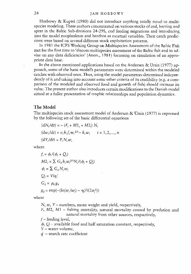
The ModelThe multispecies stock assessment model of Andersen & Ursin (1977) is expressedby the following set of the basic differential equations

(dN,/dt) = — (F1 + Mi, + M2,) N

(dw,/dt)=v,hf,w1213—kw, i= i,2,...,n

(dY/dt) = FNw

where

/= qI(4+Q,)

M2, = G,, h,w3N/( 4 + Q,)4,, = G11N1w7

Q, = VIq,

G1, =g, = exp(—(ln(w1/w,) —

i)2/(2o2))

where

N, w, Y — numbers, mean weight and yield, respectively,F, M2, Mi — fishing mortality, natural mortality caused by predation and

natural mortality from other sources, respectively,f— feeding level,4,, Q — available food and half saturation constant, respectively,V — water volume,q’ — search rate coefficient

A STOCK ASSESSMENT MODEL 25

r — positive parameter determining biomass concentration—weight relationship,v, h, k — growth parameters,

— total preference of prey i by predator j,g1 — size preference of prey i by predator j,

— food size preference parameters,p — vulnerability of prey i to predation by predator j,i, j — entity (age group or life stage),n — number of entities.

Some modifications of the Danish model were made in order to better reproduce trophic relationships. These are:

Modification of the feeding levelIn the Danish model, feeding level depends on the amount of food available topredators. Here, feeding level was modified so that it was also dependent on predator numbers. It was assumed that the search rate coefficient q, is inversely proportional to the number of fish, NSF, competing for food 4

q’ =

where is a parameter. Thus, in the present approach

Q, = q1NS

where q, = V/ce. Now the feeding level of the entity is being formulated as

f = çb1/(çb1 + qNS) = (q/NS1)/(q51/(NS + q))

depends on the available food biomass per fish competing for food c/,. Only intraspecific competition was considered and it was assumed for simplicity that, forthe given age only one year older and one year younger age groups of a speciescompete for food so

1”1S1 = A, N —1 + N + A, *1’ J\J +1

and

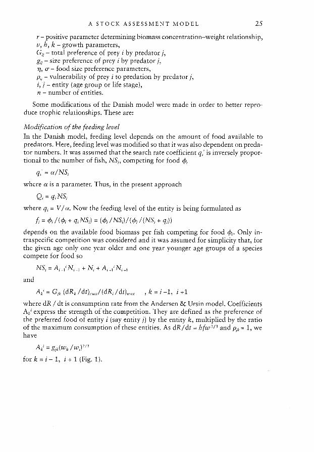
Ak1 = G1k (dRk /dt)max/(dRi /dt)max , k = i —1, i +1

where dR / dt is consumption rate from the Andersen & Ursin model. CoefficientsAk express the strength of the competition. They are defined as the preference ofthe preferred food of entity i (say entity j) by the entity k, multiplied by the ratioof the maximum consumption of these entities. As dR/dt = hfw2!3and P,k = 1, wehave

Ak’ = gJk(w /w1)213

fork=i—1, i÷l(Fig.1).

26 JAN HORBOWY

1.0

Prey biomass-dependent preference indexIvlev (1955) observed that predators can change their electivity when the biomassof prey changes. Food positively elected can be omitted when its biomass dropsmarkedly while food previously avoided can be positively elected. The analysis ofthe Baltic cod stomach contents indicates that cod increases its preference for herring when the ratio of herring to sprat biomass increases. Similarly, cod’s preferencefor zooplankton and benthos increases when the biomass of herring-like fishbiomass to cod biomass ratio declines. Thus, the cod prey biomass-dependent preference index, p, for herring, sprat, zooplankton and benthos has been modeled as

Ph f Al Th(B1,/B,—A2) + A3 for Al Th(Bh/B,—A2) + A3 i/Ph

1 l/p, for Al Th(Bh/B, — A2) + A3> i/Ph

1 for Al Th(Bh/B,—A2) +A3 i/ph

I i/[ph(Al Th(Bh/B, —A2) + A3)] for Al Th(Bh/B, — A2) + A3 > i/ph

Pb[al Th(B/(Bh + B,) —a2) + a3 for al Th(BC/(Bh + B,) —a2) + a3 Pb”

pbrnax for al Th(BC/(Bh + B,) —a2) + a3 >

PZ = Pb

B, Bh, B, — biomass of cod, herring and sprat, respectively,Al, A2, A3, al, a2, a3, pbrnx — parameters,Ph — vulnerability of herring to cod predation,Tb — tangent hyperbolic function.

.8

.6

1*1 —

‘0 .4

. 5ji-1

.2

Fig. 1. Geometrical interpretation of the sizepreference g15 included in the formula for thecoefficient Aki. W is predator weight, W isprey weight.

wi_I W. LnWia]_In— Ln__LWi Wi Wi

where


The constrains have been imposed in order to retain pp 1 (p may be greaterthan 1) and prevent too high consumption of zooplankton and benthos. NowAndersen & Ursin’s preference G1 becomes

G11 = p11 p1g11.

Mortality due to starvationAndersen & Ursin (1977) incorporated density dependent starvation mortality ofthe larval stages into their model. Here, the starvation mortality formula was developed on the basis of Ivlev’s (1955) experiments with starving fish. Ivlev examined

Table 1. Time (days) of death of 50% of bream andsheatfish fed by reduced ration r, with respect tosustained one Rs (Ivlev, 1955).

riRs Bream Sheatfish

0 34 460.1 51 760.2 73 890.4 94 1160.75 117 1421.0 126 151

the time of death of 50% of fish fed by a ration, r, reduced with respect to sustainedone, Rs (Table 1). His results can be approximated by

t50% = bl — exp(—b2 r/Rs)

where hi and b2 are parameters. Further, Ivlev states that t50% increases linearlywith fish age

tso%(t) = (bl — exp(—b2 r/Rs))(t + 1).

From the Andersen & Ursin theory, it results that

r/Rs= [Ifs

where [and fs are the actual and sustained feeding levels respectively. As fs fulfillsdw/dt=0, then

r/Rs = vhw”3f/k.

Let’s assume that the fraction, S. of death due to starvation in time zt is proportional to the length of that interval in power u. Then

S/0.5 = (t/t50%)”

and as

S = 1 — exp(— MS zt)

28 JAN HORBOWY

we have the mean in the interval zt coefficient of starvation mortality, MS

0 forffs,

MS= in 1—0.51 Zt

zt \ (bl — exp(—b2 vhw’/3f/k))(t + 1)I for f< fs and t < 2t50%,

for 1< fs and t 2/ t55%,

where 2h/II t50% is the time of the starvation death of all the fish.

External variables

The model presented has been applied in Sub-divisions 25-29S of the Baltic Properto assess predator-prey interactions and to analyze different exploitation patterns.Fig. 2 illustrates the simulated trophic levels.

CATCHES

COD

HERRING SPRAT

BENTHOS ZOOPLANKTON Fig. 2. Simulated trophic levels in Sub-divisions

_______________ _______________

25-29S of the Baltic.

To have a complete model, the author has attempted to develop submodels offish recruitment and fishing mortality. However, no distinct relationship was foundbetween cod recruitment and spawning stock biomass and data on salinity, oxygenconditions, water temperature on the spawning ground collected by the Sea Fisheries Institute. Similarly, mean fishing mortality of cod and herring appeared to beonly slightly dependent on fishing effort (determined as the ratio of the total catchto the catch per unit of effort of a selected vessel) and exploited stock biomass.Thus, recruitment and fishing mortality were treated as external variables. Theirvalues were taken from VPA results (Anon, 1986 a,b). The recruitment estimateswere then increased by multiplying them by a constant factor to compensate forhigh grazing mortality of the youngest fish. In the case of sprat, different factorswere used for the periods 1974-77 and 1978-84 to reflect low and high predatorbiomass in these periods. To reflect fishing mortality of the pre-recruit fish, meanlong-term partial recruitment coefficients were used.


Zooplankton and benthos were also treated as external variables. Their meanyearly values for 1974-79 (Table 2) were estimated by Horbowy & Kuptel (1980based on the Sea Fisheries Institute’s data on zooplankton and benthos distributionin the Gulf of Gdansk and the estimate of long-term production of zooplanktonand long-term benthos biomass (Thurow, 1978)). For the 1980-84 period, average

Table 2. Mean yearly biomass (106 tons> of zooplankton and benthos used in the model.

Year 1974 1975 1976 1977 1978 1979 1980-84

Zooplankton 4.4 4.4 4.8 4.0 5.4 5.1 4.7Benthos 2.8 2.9 3.0 2.7 3.2 3.3 3.0

values were used as there is a lack of appropriate yearly data. Each month, a newbiomass of zooplankton and benthos is introduced into the model on the basis oftheir monthly distribution in the Gulf of Gdansk (Horbowy & Kuptel, 1980); theweight of the individuals present remains constant.

Parameter values

The parameter values are presented in Table 3. The food preference parameters forcod were determined on the basis of cod stomach contents data (Zalachowski, inpress); these data were also submitted to the Working Group on MultispeciesAssessments of Baltic Fish. For the i, cr and p values, the method of Ursin (1973)slightly modified by Horbowy (1982) was used. Parameters Al, A2, A3, al, a2, a3were adjusted so as to give simulated p values close to the observed (Fig. 3). In orderto determine the observed p values the p estimates for each year were obtained bythe method cited above. Next it was assumed that the variance in the p values iscaused by the p values contained in them, so the observed p’s were estimated fromthe formula

PVy=Y

iJ ) 6J

where p is mean vulnerability for the 1977-84 period and y denotes a year. The ,o- and p values for herring and sprat were assumed.

To determine growth parameters, von Bertalanffy’s equations were fitted toweight-at-age data (Anon., 198 6a,b). Weight-at-age estimates for herring and sprat

3 3

herring benthos

Fig. 3. Modeled prey bio-2 2

mass-dependent preference index, p,,, versus oh-

°served one, P055 for twocod preys: herring andbenthos.

1 2 3 4 1 2 3

® omitted P ohs

30 JAN HORBOWY

Table 3. Values of parameters used in the model.

Parameter Age group Cod Herring Sprat

v 0.3 0.3 0.3h 18.7 27.0 10.2k 0.023 1.3 0.93

0 27 225 201 20 59 82 50 97 163 74 121 28

q 4 169 161 565 600 231 866 1750 341 2007 4400 451 5948 11000 501 —

Thod 3.6 — —

7hcrrng 4.15 — —

Thp 4.55 — —

1bcnthos 6.1 5.9 —

7Izooplnkton 5.0 5.9 5.6

°od 1.05 — —

hring 0.76 — —

Uspra 1.0 — —

0bcntho 0.25 0.02LTzooplankton 0.15 0.02 0.15

Pd 0.5 — —

Pherring 0.6 — —

Psprn 1.0 — —

Pbnntho 0.42 1.0 —

Pnooplnnkron 0.046 1.0 1.0

Al 0.36A2 4.4A3 1.2al 2.4a2 0.25a3 0.8

Mi 0.25 0.15 0.1561 1.1 1.1 1.1b2 0.33 0.33 0.33u 2.0 2.0 2.0

in Sub-divisions 25-29S were determined as the weighted by numbers mean weightat-age of appropriate populations (herring in Sub-divisions 25-27 and 28-29S, andsprat in Sub-divisions 25, 26 + 28 and 27 + 29S). Next, the v value taken fromJobling (1982) was used to calculate


for i belonging to a species and H being the anabolism coefficient in von Bertalanffy’s equation. The above simultaneous equations served for the estimation ofq values. The number of unknown parameters (q1 and h) is greater by 1 than thenumber of equations, so h was chosen in such a way as to give the best correspondence of the observed and simulated in the model growth of fish.

The values of bi and b2 were determined on the basis of Ivlev’s (1955) experiments (Table 1). Mi was adjusted so as to give M for adult fish similar to the valuesassumed by the Baltic Working Groups.

Results and DiscussionReliability of the modelThe mean relative differences between the simulated and observed catches of cod,herring and sprat were 10, 9 and 12%, respectively (Table 4). At least part of thatdifference is caused by the mean long-term partial recruitment coefficients used inthe model. For example, employing actual partial recruitment coefficients for codin 1977 would reduce the difference for that year from —27% to —7%.

Table 4. The relative difference between the catches(in weight) determined by the multispecies modeland the observed catches from Working Group reports for 1974-1984 period (in %).

Year Cod Herring Sprat

1974 —1 —13 —131975 18 —6 31976 —14 14 61977 —27 5 81978 —1 12 —111979 10 6 —111980 —6 10 —231981 —15 —12 —141982 —4 10 —171983 6 9 21984 5 —5 21

Mean of absolute values 10 9 12

Age group Cod Herring Sprat

0 — 0.23 —0.051 0.33 0.40 0.892 —0.02 0.59 0.853 0.56 0.79 0.964 0.95 0.88 0.945 0.92 0.72 0.936 0.92 0.78 0.897 0.93 0.97 —

A comparison of the age composition of cod, herring, and sprat catches, calculated by means of the model, with the observed age composition is presented inTable 5. Correlation coefficients between observed and calculated catches are highin most cases. Greater deviations may be observed mostly in partially recruited agegroups. For cod, this may be seen in age groups 1 and 2, for herring — in age groups0 and 1, for sprat — in age group 0. These differences are the result of causes discussed above — the use of mean long-term partial recruitment coefficients. As a re

Table 5. The correlation coefficients betweencatch at age in numbers estimated by the modeland observed one in 1974-1984.

32 JAN HORBOWY

500r 700 1000Age 2 Age3 Age 4

r= .53 r .40 r

300[ 600 900

I 0© omitted

0 © 000

200 400 000 © 8000

2 34 36 40 42 46 48

2200 00

3200

Ages 0

1600 r= .77 2000 03000

1400•

1800 02803 Fig. 4. Correlation be-

0 0 tween the weight of0 Age 7 cod determined by the

© r=1200 1600 2600 model, torn, and obAge 6 served length, 1obs’ by

- .24age groups 2-7 in

54 56 62 641974-84 years.

obs (Cm)

suit, there is a certain error in those years, in which deviations of the coefficientsfrom their mean values are quite large.

Weight of cod by age groups simulated in the model is in fairly good agreementwith cod lengths observed in the catches (Fig. 4). Observed length (Kosior, pers.communication) instead of observed weight was used for comparison because of itsbetter availability and greater accuracy. The highest correlation coefficients between calculated and observed values were obtained for cod age groups 4, 5 and 7(about 0.8), lower for age groups 2 and 3 (0.63 and 0.40 respectively). Cod agegroups 2 and 3 are not fully recruited to the exploitable stock so only larger specimens from these groups are caught. This may be the cause of poor correlation between their simulated and observed growth. The model did not reflect the growthof the cod age group 6. The reason for that may be low variation in the observedvalues.

A comparison of growth of herring and sprat calculated from the model with theobserved growth is somewhat difficult since the model use simulated herring andsprat stocks from Sub-divisions 25-29S while available data refer to growth observed in actual stocks. Grygiel (1979) presented the mean weight of sprat in thesouthern Baltic by age groups for the 1974-1977 period. When these data werecompared with the values obtained from the model, a rather good relationship wasobtained (Fig. 5). The adequacy of the herring growth equation used in the modelmay be argued on the basis of Horbowy (1983). Using a herring growth equation

Fig. 5. Correlation between themodeled, Wm and observed,W0b,, weight of sprat by agegroups 0-5 in 1974-1977 years.

Fig. 6. Correlation between theshare of sprat, herring and zoo-plankton + benthos in the cod’sfood determined on the basis ofthe model, F,,,, and observedshare, 1obs’ by cod’s age groups2-6 in 1977-1984 years.

2 4 6 8 10 12 14 16

spratr* .58

XX

IC

6,,

X% X

W (giohs

zaoplanktan * benthosr= .51

0 Omitted

* ageS

o age 4-5

x age 3

• age 2

33

r* .68

A STOCK ASSESSMENT MODEL

r= .76

r*.74

XX

r= .55

0

rc-.05

0

a

a age 0

5—”— 1o —ii— 2*_,_ 30-- 4

5

12

10

0

8

6

20

80

60

40

60 herringr*.82

40 *

00

Xc20

)S<X XXX

P (‘I,,)obs

0

20 40 6020 40 60

0

XX

0 0

0*

0

* 5 *0*00

S

20

20 40 60

p (*/)ohs

80 103

34 JAN HORBOWY

similar to that used here, the author obtained good comparability between the calculated length and the observed.

The last criterion of the model’s reliability consisted of a comparison of the simulated and observed species composition of the food of cod. Only the food of codwas considered since the food of herring and sprat was treated in the model in avery general way (zooplankton as a whole and benthos as a whole). The observedcomposition of cod food (Zaachowski, in press) is presented by 5- and 10-cmlength classes. On the other hand, the model is based on the use of age groups andall calculations are made for them. Thus, to enable a comparison of the calculatedfood composition with the observed, age groups were assigned to all length intervalsfrom the data of Zafachowski. This procedure resulted in a certain error in the obtained data observed by age group since individual age groups did not correspondexactly to the length classes according to which Zalachowski classified his data.Nevertheless the correlation between the simulated and observed food compositionof cod split into herring, sprat, and zooplanktori + benthos (Fig. 6) was fairly satisfactory. It is worth noting that the model reflects relatively well changes in the shareof sprat in the food of individual cod age groups and — to a lesser degree — the shareof zooplankton + benthos in the food of age groups 3 and 4-5 in consecutive years.The model did not reflect the variance of the observed share of herring in the foodof various age groups of cod. This may have been caused by a lower variance in thisshare when compared with sprat and zooplankton + benthos.

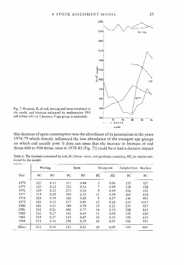
Stock dynamics in the 1974-1984 periodBiomass values simulated in the model for cod, herring, and sprat stocks in the1974-84 period are shown in Fig. 7. For comparison, biomass estimates of thesespecies made by the Baltic multispecies Working Group (Anon., 1988) are presentedas well. All presented values refer to 1 January. Herring biomass estimates from themodel are very close to the multispecies Working Group values while the simulatedbiomass of sprat exhibits a similar trend to the multispecies Working Group estimates with an increasing difference from 1981-84. The MSVPA values of predationmortality were in the range of 1.0-1.8 for many age groups of sprat from Sub-division 25. This is about 3 times higher than the model estimates. The biomass estimates of cod also show a similar trend to the MSVPA values. However, MSVPA values are about 50% greater than the model estimates. This difference was primarilycaused by the cod’s weights-at-age which, in the MSVPA, are 200-50% higher forthe 2-4 age groups respectively than those simulated in the model. These age groupsconstitute about 50% of cod biomass and the weights-at-age used in the MSVPAare weights-at-age in the catch, which may result in overestimation of MSVPAbiomass.

The consumption of herring-like fish by cod in 1974-84 estimated by the modelwas, on average, about 550 thous. tons (410 to 760 thous. tons (Table 6)). This figure included, on the average, 210 thous. tons of herring (120-290 thous. tons range)and 335 thous. tons of sprat (190-540 thous. tons range). In the 1976-79 period,the consumption of sprat by cod kept decreasing, being compensated for by increasing consumption of benthos (as high as 900-1000 thous. tons). The main reason for


2000 herring

1800

o’:=t

(all values refer to 1 January, 0 age group is excluded).2ooi.-

76 78 80 82 84MSVPA

model

this decrease of sprat consumption was the abundance of its generations in the years1976-79 which directly influenced the iow abundance of the youngest age groupson which cod usually prey. It does not seem that the increase in biomass of cod(from 600 to 900 thous. tons in 1978-83 (Fig. 7)) could have had a decisive impact

Table 6. The biomass consumed by cod, BC (thous. tons), and predation mortality, M2, by species estimated by the model.

Herring Sprat Young cod Zooplankton Benthos

Year BC M2 BC M2 BC M2 BC BC

1974 117 0.11 311 0.44 5 0.06 135 4271975 152 0.13 333 0.52 7 0.09 158 4381976 159 0.13 273 0.50 9 0.09 236 5311977 219 0.20 203 0.55 11 0.09 263 6181978 228 0.19 186 0.69 9 0.07 236 8951979 285 0.25 217 0.84 12 0.10 235 10371980 282 0.23 340 0.78 15 0.12 234 9271981 241 0.21 406 0.77 14 0.10 208 8141982 216 0.17 543 0.64 11 0.08 150 6501983 219 0.17 514 0.69 10 0.10 150 6121984 215 0.16 358 0.59 10 0.09 182 591

Mean 212 0.18 335 0.63 10 0.09 199 685

36 JAN HORBOWY

Table 7. Mean biomass consumed by cod (thous. tons)by age groups in 1974-19 84 estimated by the model.

Cod Prey speciesage Zoo-

group Herring Sprat Benthos plankton

0 0 0 13 901 3 25 115 842 21 83 180 203 47 125 164 44 52 70 110 15 39 23 56 06 24 7 26 07 14 2 12 08+ 12 0.5 9 0

Table 8. Biomass (thous. tons) of herringand sprat consumed by cod in 1980-1984estimated by the multispecies VPA (Anon.,1988).

Herring Sprat 25,Year 25-29S 26+28

1980 775 1871981 856 6641982 810 8211983 677 9431984 583 663

on the low recruitment of sprat. This argument is supported by the fact that thenumbers of recruited herring, which are also eaten intensively by cod, did not undergo great fluctuations. In the 1980-1984 period, a large increase in the consumption of sprat, thus, reflecting an increase in its biomass, was observed. This was accompanied by a decrease in benthos consumption.

Cod from age groups 2-4 eat, on average, 280 thous. tons of sprat. This constitutes 83% of the sprat biomass consumed by all predators (Table 7). Herring aremostly consumed by cod age groups 3-5 and the amount consumed is 140 thous.tons, which constitutes 65% of herring biomass lost to predation.

Let us also compare the consumption by cod calculated by means of the modelwith multispecies VPA estimates made in Anon. (1988), (Table 8). The cod’s consumption of herring assessed by the Baltic multispecies Working Group is about 3times greater than the model estimates (Table 6) while cod’s consumption of spratexceeds the model values by about 50%. The MSVPA simulations are based on theannual consumption by cod calculated using the evacuation rate for North Sea cod(24 hours). However, in situ estimation of the evacuation time of sprat from codstomachs in Sub-divisions 25 indicated a period of 60-70 hours (Anon., 1988).Applying this value in the calculations, would reduce the biomass of sprat consumed by cod estimated in MSVPA by about a factor of 3. Taking into account inMSVPA, sprat from Sub-divisions 27 and 29S could produce a value for spratbiomass eaten by cod, which is close to the model estimates. Assuming that theevacuation time for herring in cod stomachs is similar to that for sprat, then theherring biomass consumed by cod assessed by MSVPA would also decrease by afactor of about 3 and would be very close to the model estimates. Some differencesbetween the estimates of cod consumption may be caused by basing the model onPolish stomach content data only while the MSVPA runs employ both Polish andUSSR data which are different.

The entire sprat stock, 0-1 age groups of herring and the 0 age group of cod sustain the heaviest predation by cod (Table 9). The other fish are consumed to a smalldegree.


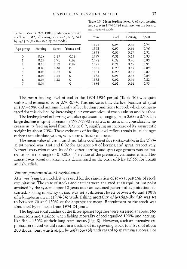
Table 9. Mean (1974-1984) predation mortalitycoefficient, M2, of herring, sprat and young codby age groups estimated by the model.

Age group Herring Sprat Young cod

0 0.28 0.69 0.181 0.24 0.71 0.082 0.13 0.52 0.023 0.08 0.40 04 0.06 0.32 05 0.04 0.28 06 0.04 0.25 07 0.04 — 0

Table 10. Mean feeding level, / of cod, herringand sprat in 1974-1984 estimated on the basis ofmultispecies model.

Year Cod Herring Sprat

1974 0.94 0.66 0.741975 0.93 0.66 0.761976 0.93 0.67 0.811977 0.91 0.63 0.831978 0.92 0.70 0.891979 0.91 0.69 0.911980 0.90 0.67 0.891981 0.90 0.67 0.871982 0.91 0.67 0.841983 0.92 0.66 0.821984 0.92 0.66 0.83

The mean feeding level of cod in the 1974-1984 period (Table 10) was quitestable and estimated to be 0.90-0.94. This indicates that the low biomass of spratin 1977-19 80 did not significantly affect feeding conditions for cod, which compensated for this decline by increasing their consumption of zooplankton and benthos.

The feeding level of herring was also quite stable, ranging from 0.63 to 0.70. Thelarge decline in sprat biomass in 1977-1980 resulted, in turn, in a considerable increase in its feeding level from 0.75 to 0.9, signifying an increase of its asymptoticweight by about 70%. These estimates of feeding level reflect trends in its changesrather than absolute values, which are difficult to assess.

The mean value of the natural mortality coefficient due to starvation in the 1974-1984 period was 0.04 and 0.02 for age group 0 of herring and sprat, respectively.Natural starvation mortality of the other herring and sprat age groups was estimated to be in the range of 0-0.003. The value of the presented estimates is small because it was based on parameters determined on the basis of Ivlev (1955) for breamand sheatfish.

Various patterns of stock exploitationAfter verifying the model, it was used for the simulation of several patterns of stockexploitation. The state of stocks and catches were analysed at an equilibrium pointattained by the system about 10 years after an assumed pattern of exploitation hasstarted. Fishing mortality of cod was set at different levels between 40 and 190%of a long-term mean (1974-84) while fishing mortality of herring-like fish was setto between 70 and 130% of the appropriate mean. Recruitment to the stock wassimulated by its mean from 1974-84 years.

The highest total catches of the three species together were assessed at about 665thous. tons and attained when fishing mortality of cod equalled 190% and herring-like fish — 130% of their long-term means (Fig. 8). However, such an intensive exploitation of cod would result in a decline of its spawning stock to a level of about200 thous. tons, which might be unfavourable with regard to spawning success. For

38 JAN HORBOWY

800A

400B

x X X 0

600 0 0 3(0 7QCx x

— x 0

.400 200 x

600

200 100

Fcod

•Fhs • sprot 1=3, Fh= F

oFhs - F o herring,

F, x F1,,= 1.3

x F = 1.3 x cod • I‘ F,5 F

hos+ IC

= 13

• t =5 F-,5= 1.3=

Fig. 8. A. Total catches for different fishing mortality of cod Fd, and herring-like fish, F+h. B. Catchesby species for different FCOd . C. Total catches for different F0d and Fh+, and age of full capture of cod,t (the unit of fishing mortality is the long-term mean fishing mortality).

this reason the variant according to which cod fishing mortality should increase by60% should be considered to give maximum yield. This enables a catch of 660thous. tons of fish, including 265 thous. tons of cod and 395 thous. tons of herringand sprat. Such catches would be higher by 15 thous. tons than those attained atan exploitation intensity of cod equal to the long-term mean. At the same time, thecost of cod catches would increase significantly because of the great decline of itsbiomass and related drop in the catch per effort. The simulations also indicate theoverfishing of cod. A decrease of fishing intensity to 70% of its long-term meanwould enable a slight increase of cod catches and a concomitant reduction of costs.Other simulations were made in order to assess the impact of both abandoning fishing operations for cod and the elimination of cod from the ecosystem on stocks andcatches. In the first case, total catches dropped considerably (to 200 thous. tons).This figure included 164 thous. tons of herring and 37 thous. tons of sprat.

The problem of the state of stocks after eliminating the cod population is farfrom simple since, as the result of the lack of natural mortality due to predation M2,natural mortality Mi would probably increase (the predator eliminates weaker anddiseased individuals). We are unable to estimate this change.

Employing in the calculations the hitherto used values of Mi, the total catchafter eliminating cod stock and maintaining fishing intensity for herring and spratat unchanged levels equalled 510 thous. tons (herring — 270 thous. tons, sprat —

230 thous. tons). However, due to their overabundance, these fish would be small,weights of sprat would not exceed 6g, weights of herring — 40g. Increasing fishingmortality for herring-like fish up to 3 times the mean value would allow for catch-


ing 920 thous. tons of fish (herring — 560 thous. tons, sprat — 360 thous. tons) ofnormal size.

Assuming that Mi increases to the currently assumed value of total natural mortality for adults (M = 0.2 for herring, M = 0.5 for sprat) then by increasing fishingmortality of herring and sprat 3 times, we would have a catch of 700 thous. tons(500 thous. tons of herring, 200 thous. tons of sprat).

The actual catch after eliminating cod would probably be contained somewherewithin these levels, determined by extreme values of Mi. However, these considerations do not take into account positive effects of predator presence (e.g. a decreasein the fluctuations of prey population biomass, elimination of weaker and diseasedindividuals).

The next simulation involved the influence of a change of the age of full captureof cod on the catches attained, with the fishing mortality for herring-like fish equalto the long-term mean and 30% higher than the mean, and employing various levelsof fishing mortality for cod (Fig. 8). The most favourable results were obtainedwhen the age of full capture of cod was reduced from the current 4 to 3 years andfishing mortality for cod, herring and sprat was increased by 30%. The catch attained at this variant would be about 670 thous. tons (230 thous. tons of cod and440 thous. tons of sprat and herring), i.e. higher by 10 thous. tons than in the bestvariant maintaining the present age of full capture of cod. A further increase in fishing mortality of cod would result in a decline of the biomass of its spawning stockbelow 200 thous. tons. A variant involving an increase of the age of full capture ofcod to 5 years and a simultaneous large (90%) increase of its fishing mortality (intensive catch of older fish, feeding mainly on herring-like fish) turned out to be unfavourable. There were two reasons for this. First, a greater part of the consumedbiomass of sprat and herring is eaten by cod in age groups 2-5 (Table 7). Second,this variant does not lead to a sufficient decrease of cod biomass due to their beingcaught so late.

The simulations carried out point to a moderate sensitivity of total catches tochanges in fishing intensity of cod ranging from 40 to 190% of their long-termmean. Their increase is about 70-120 thous. tons, a result of an increase in codcatches by about 35 thous. tons. Only the total elimination of cod has a visible impact on the yield obtained. Although the biomass of herring and sprat consumed bycod seems moderate it consists mainly of young fish. As a result, cod eliminatesabout 50% of sprat in age group 0 and 25% of the same age group of herring.

The dependence of the biomass of the herring-like fish on the biomass of cod(Fig. 9) resembles a power relationship (linear on the logarithmic scale). An increasein cod stock biomass c times results in a decrease of herring and sprat biomass byabout g times. The influence of herring and sprat biomass on cod biomass is muchsmaller in the biomass range taken into account here. A decrease in herring andsprat stock by 10% brings about a decline in cod biomass by about 1% and is practically not reflected in the catches.

40 JAN HORBOWY

80 .

7.8 x

7.4

7.2•

F,,5 = 03 FFig. 9. The relationship between herring

F like fish biomass, B5,, and cod biomass B,X F

:= 1.3 F for three levels of herring and sprat fishing

70 .., mortality, Fh,S.70 80

In B

Discussion of modifications testedLet us analyse the advisability and effect of the modifications introduced into theDanish model on the basis of the results of simulations and literature. The direct introduction of the abundance of fish competing for food, NS, to the denominator ofthe formula for feeding level is justified by the experiments of Houde (1975, 1977).He found that the growth rate and survival of sea bream, bay anchovy and linedsole larvae were negatively correlated with population density. The dependence ofgrowth on population density resembled the hyperbolic function used here to describe feeding level. In addition, Horbowy (1983) presented a model of Baltic herring growth, in which relating feeding level to the number of fish made it possibleto reflect the observed growth.

The influence of the introduction of a food preference coefficient dependent onthe biomass of prey, p, may be well seen by comparing the growth of cod age groups4 and 5, obtained from two models (Fig. 10). A sudden decline in the sprat stockbiomass in 1977-1979 (in Fig. 7 the lowest sprat biomass is in 1980 but it does notinclude the 0 age group which was very abundant in that year) was immediately reflected in the growth of these two age groups calculated with the help of the unmodified model. In the case of the modified model, cod compensated for the scarcityof sprat by increasing consumption of zooplankton and benthos. As a result of this,growth of cod was similar to that observed. Feeding on sprat is much less importantfor cod in age groups 6 and 7 and for these groups, both models give a qualitativelysimilar picture of predator growth to that observed. As a result, the modified formof f and the introduction of coefficient p led to a much higher correlation betweencalculated cod growth and that observed (Table 11). The present model also betterreflects the growth of sprat (Table 11).

The accuracy of the formula for natural mortality due to starvation introducedhere may be discussed only on the basis of literature as appropriate data are notavailable. Ursin (1967) determined the catabolism coefficient for Lebistes reticula


49 1000 57 1700

Age S

48 900

Age

56 1500

47 801 1300

— St— 74 76 78 80 74 76 78 80

72 3000

Age 6 73 320065 2403

64 2200

Fig. 10. Cod growthin weight simulated

_

e7

in the unmodified 63 2000 71 2800

model (A), in themodified model (B),and the observed 62 1800 2600

growth of cod inlength in 1974-1980

______________________

SCyears. 74 76 78 80 74 76 78 80years

o—o observedX—3< model B— model A

tus, observing that until the fish lost 20% of their weight, mortality was low andthen rapidly increased. This seems to be in agreement with MS treated as a functionof &, which first increases slowly and then rapidly. Laurence (1974) investigatedthe growth and mortality of haddock larvae depending on the amount of food. Heobtained a high correlation between growth and survival rate of larvae and amountof food available to one larva, 4/N. The dependence of mortality on 4/N is similarto the relationship between presented here for the functional form of MS and /N.Mills (1982) analysed factors influencing the mortality and growth of dace larvae.

Table 11. The correlation of the fish growth determined by the unmodified model (a) andmodified model (b) with the observed growth.

Age groupSpecies 1 2 3 4 5 6 7

a — —0.19 0.55 0.55 0.40 0.20 0.18Cod

b — 0.63 0.40 0.91 0.77 0.24 0.79

a —0.57 —0.39 0.36 0.88 0.54 — —

Spratb 0.74 0.76 0.81 —0.05 0.68 — —

42 JAN HORBOWY

It turned out that growth rate was smaller and mortality greater in tanks with agreater number of larvae. Changes in mortality due to the abundance of larvae weresimilar to changes of MS as a function of N. The investigations carried out byWerner & Blaxter (1982) on the influence of food on the growth and survival rateof herring larvae showed that both processes depend on the amount of food andchanges in mortality were qualitatively similar to the changes of MS.

AcknowledgementsI would like to thank K.P. Andersen and Dr. E. Ursin for their valuable comments on earlier draft of thepresent paper. I am grateful to Dr. M. Kosier for placing at my disposal partly unpublished data on codlength. Reports of ICES Working Groups are quoted by kind permission of the ICES General Secretary.

ReferencesAndersen, K.P., Ursin, E. 1977. A mulrispecies extension to the Beverton and Holt theory of fishing with

accounts of phosphorus circulation and primary production. — Meddr Danm. Fisk- og Havunders.N.S. 7: 31.9-435.

Anon., 1981. Report of the ad hoc Working Group on multispecies assessment in the Baltic. — ICES C.M.1 981/J:34.

Anon. 1986a. Report of the Working Group on the assessment of the demersal stocks in the Baltic. —

ICES 1986/Assess.: 21.Anon. 1986b. Report of the Working Group on the assessment of the pelagic stocks in the Baltic. — ICES

1986/Assess.: 20.Anon. 1988. Report of the Working Group on multispecies assessments of Baltic fish. — ICES

1988/Assess.: 1.Grygiel, WY. 1979. Wzrost szprota poludmowego Baltyku. (The growth of sprat in the southern Baltic).

— In: Z biologii ryb Baltyku. Studia i materialy. Ser. B144.Horbowy, J. 1982. The estimation of parameters of predator-prey preference function for Baltic cod. —

ICES 1982/J:28.Horbowy, J. 1983. The modeling of the coastal spring herring growth and modified yield per recruit

curve. — ICES 1983/J:5.Horbowy, J., Kuptel, M. 1980. Use of a multispecies model to assess Baltic stocks and forecast catches.

— ICES 1980/J:15.Houde, E.D. 1975. Effects of stocking density and food density on survival, growth and yield of labo

ratory-reared larvae of sea bream Archosargus rhomboidalis (L), (paridae). —J. Fish. Biol. 7: 115-127.

Houde, E.D. 1977. Food concentration and stocking density effects on survival and growth of laboratory-reared larvae of bay anchovy Anchoa mitchili and lined sole Achirus lineatus. — Marine Biology.43: 333-341.

mien, vs. 1955. Eksperimentalnaja ekologia pitanija ryb. (Experimental ecology of fish feeding). —

Naukova dumka. Kiev.Jobling, M. 1982. Food and growth relationship of th cod, Gadus rnorbua L., with special references to

Balsfjorden, north Norway. —J. Fish. Biol. 21: 357-371.Laurence, G.C. 1974. Growth and survival of haddock (Melanogrammus aeglefinusl larvae in relation

to planktonic prey concentration. —J. Fish. Res. Bd. Can. 31: 1415-1419.Majkotuski, J. 1977. Prognosis for catches of cod, herring and sprat in the Baltic Sea, and their optimiza

tion with the aid of the mathematical model. — Pol. Arch. Hydrobiol. 24: 361-382.Mandecki, WY. 1976. A computer simulation model for interacting fish populations studies, applied to

the Baltic. — Pol. Arch. Hydrobiol. 23: 281-307.Mills, CA. 1982. Factors affecting survival of dace, Leuciscus leuciscus (L.), in the early post-hatching.

— J. Fish Biol. 20: 645-655.


Thurow, ER. 1978. The fish resources of the Baltic Sea. — FAO Fish. Circ. No. 708.Ursin, E. 1967. A mathematical model of some aspects of fish growth, respiration and mortality. J. —

Fish. Res. Bd. Can. 24: 2355-2453.Ursin, E. 1973. On the prey size preference of cod and dab. — Meddr Danm. Fisk- og Havunders. 7: 85-

98.Werner, R.G., (Clupea harengus) in relation to prey density. — Can. J. Fish. Res. Aquatic Sci. 37: 1063-

1069.Zaachowski, W. Feeding of cod in southern Baltic in 1977-1984. — In ICES Cooperative Research

Report (in press).

Documents

A multispecies model of fish stocks in the Baltic Sea