A Multiscale Mortar Multipoint Flux Mixed Finite Element Method

Mary F. Wheeler ∗ Guangri Xue † Ivan Yotov ‡

Abstract

In this paper, we develop a multiscale mortar multipoint flux mixed finite element method for secondorder elliptic problems. The equations in the coarse elements (or subdomains) are discretized on a finegrid scale by a multipoint flux mixed finite element method that reduces to cell-centered finite differenceson irregular grids. The subdomain grids do not have to match across the interfaces. Continuity of fluxbetween coarse elements is imposed via a mortar finite element space on a coarse grid scale. With anappropriate choice of polynomial degree of the mortar space, we derive optimal order convergence on thefine scale for both the multiscale pressure and velocity, as well as the coarse scale mortar pressure. Somesuperconvergence results are also derived. The algebraic system is reduced via a non-overlapping domaindecomposition to a coarse scale mortar interface problem that is solved using a multiscale flux basis.Numerical experiments are presented to confirm the theory and illustrate the efficiency and flexibility ofthe method.

keywords. multiscale, mixed finite element, mortar finite element, multipoint flux approximation, cell-centered finite difference, full tensor coefficient, multiblock, nonmatching grids, quadrilaterals, hexahedra.

1 Introduction

We consider a second order linear elliptic equation written in a mixed form. Introducing a flux variable, wesolve for a scalar function p and a vector function u that satisfy

u = −K∇p in Ω, (1.1)

∇ · u = f in Ω, (1.2)

p = g on ∂Ω, (1.3)

where Ω ⊂ Rd, d = 2, 3, is a polygonal domain with Lipschitz continuous boundary and K is a symmetric,

uniformly positive definite tensor with L∞(Ω) components, satisfying, for some 0 < k0 ≤ k1 <∞,

k0ξT ξ ≤ ξTK(x)ξ ≤ k1ξ

T ξ ∀x ∈ Ω ∀ξ ∈ Rd. (1.4)

We assume that f ∈ L2(Ω) and g ∈ H1/2(∂Ω). The choice of Dirichlet boundary condition is made forsimplicity. More general boundary conditions can also be treated. In porous media applications, the system(1.1) – (1.3) models single phase Darcy flow, where p is the pressure, u is the velocity, and K represents therock permeability divided by fluid kinematic viscosity.

∗Center for Subsurface Modeling (CSM), Institute for Computational Engineering and Sciences (ICES), The University ofTexas at Austin, Austin, TX 78712; mfw@ices.utexas.edu; partially supported by the NSF-CDI under contract number DMS0835745, the DOE grant DE-FG02-04ER25617, and the Center for Frontiers of Subsurface Energy Security under Contract No.DE-SC0001114.

†(CSM), (ICES), The University of Texas at Austin, Austin, TX 78712; gxue@ices.utexas.edu; supported by Award No.KUS-F1-032-04, made by King Abdullah University of Science and Technology (KAUST).

‡Department of Mathematics, University of Pittsburgh, Pittsburgh, PA 15260; yotov@math.pitt.edu; partially supportedby the DOE grant DE-FG02-04ER25618, the NSF grant DMS 0813901, and the J. Tinsley Oden Faculty Fellowship, ICES, TheUniversity of Texas at Austin.

1

To alleviate the computational burden due to the solution dependence on a large range of scales, amultiscale mortar mixed finite element method for the the numerical approximation to (1.1)–(1.3) wasdeveloped in [9], using mortar mixed finite elements [7] and non-overlapping domain decomposition [32]. Inthis paper we develop a new multiscale mortar mixed method that uses the multipoint flux mixed finiteelement (MFMFE) [53, 37] for subdomain discretization.

The MFMFE method was motivated by the multipoint flux approximation (MPFA) method [4, 5, 25, 26].The latter method was originally developed as a non-variational finite volume method. It is locally massconservative, accurate for rough grids and coefficients, and reduces to a cell-centered system for the pressures.In that sense it combines the advantages of MFE and several MFE-related methods.

MFE methods [19, 46] are commonly used for flow in porous media, as they provide accurate and locallymass conservative velocities and handle well rough coefficients. However, the resulting algebraic systemis of saddle point type and involves both the pressure and the velocity. Various modifications have beendeveloped to alleviate this problem, including the hybrid MFE method [12, 19] that reduces to a symmetricpositive definite face-centered pressure system, as well as more efficient cell-centered formulations basedon numerical quadrature for the velocity mass matrix in the lowest order Raviart-Thomas [49, 45, 44](RT0) case [47, 51, 10, 8, 13]. In terms of efficiency, the cell-centered methods are comparable to the finitevolume methods [28]. All of the above mentioned cell-centered methods exhibit certain accuracy limitations,either in terms of grids or coefficients (full tensor or discontinuous). Two other family of methods that areclosely related to the RT0 MFE method and perform well for rough grids and coefficients are the controlvolume mixed finite element (CVMFE) method [21] and the mimetic finite difference (MFD) methods [36].However, as in the case of MFE methods, both methods require solving algebraic saddle point problems intheir standard form.

The MPFA method handles accurately very general grids and discontinuous full tensor coefficients andat the same time reduces to a positive definite cell-centered algebraic system for the pressure. The analysisof the MPFA method has been done by formulating it as a MFE method with a special quadrature, see[53, 39] for the symmetric version on O(h2)-perturbations of parallelograms, [40] for non-symmetric versionon general quadrilaterals, and [52] for non-symmetric version on general hexahedra. A non-symmetric MFDmethod on polyhedral elements that reduces to a cell-centered pressure system using a MPFA-type velocityelimination is developed and analyzed in [42].

Here we use for subdomain discretizations the MFMFE method developed in [53] for simplicial elementsand quadrilaterals and extended in [37] to hexahedra, see also closely related method on simplicial elements[20]. Since the MPFA method uses sub-edge or sub-face fluxes to allow for local flux elimination, theMFMFE method is based on the lowest order Brezzi–Douglas–Marini space, BDM1 [18], and its extension tohexahedra, BDDF1 [17, 37], which have similar velocity degrees of freedom. The BDDF1 space was enhancedin [37] with six additional curl basis functions. The resulting space has bilinear normal traces on the faces,thus four degrees of freedom per face, which allows for a MPFA-type local velocity elimination. This is donevia a special quadrature rule for the velocity mass matrix that reduces it to a block-diagonal form, withblocks corresponding to the mesh vertices. As a result, the velocity can be easily eliminated, leading to acell-centered system for the pressure.

The permeability K in (1.2) is usually highly heterogeneous and varies on a multiplicity of scales. Re-solving the solution on the finest scale is often computationally infeasible, necessitating multiscale approx-imations. In this paper we develop a new multiscale mortar MFMFE method. The approach is similarto the one in [9] for the multiscale mortar mixed finite element method. The latter was developed as analternative to existing multiscale methods, such as the variational multiscale method [35, 6] and multiscalefinite elements [34, 22, 38, 2, 1]. In the multiscale mortar approach, the domain is decomposed into a seriesof small subdomains (coarse grid) and the solution is resolved globally on the coarse grid and locally (oneach coarse element) on a fine grid. We allow for geometrically nonconforming domain decompositions andnon-matching grids across the interfaces. Continuity of flux is imposed weakly using a low degree-of-freedommortar space defined on a coarse scale mortar grid. Mortar methods were first introduced in [14] for Galerkinfinite elements. In this paper we consider the MFMFE method for subdomain discretizations. In this con-text, special care needs to be taken in imposing weak flux continuity through the mortar space. In particular,

2

the method requires that the jump of the RT0-projections of the BDM1 or BDDF1 fluxes be orthogonal tothe mortar space. This condition is needed to ensure stability and accuracy of the method.

We solve the algebraic system resulting from the multiscale mortar MFMFE method via a non-overlappingdomain decomposition algorithm [32, 7, 9]. By eliminating the subdomain unknowns, the global multiscaleproblem is reduced to a coarse interface problem, which is solved using an iterative method. Employingthe approach from [30], we precompute a multiscale flux basis by solving in each subdomain Dirichlet finescale local problems for each mortar degree of freedom associated with that subdomain. The subdomainproblems are easy to solve due to their relatively small size. Furthermore, this is done in parallel without anyinterprocessor communication. Computing the action of the interface operator on every interface iterationis then reduced to a linear combination of the multiscale flux basis. The resulting method combines theefficiency of the multiscale mortar methodology with the accuracy and flexibility of the MFMFE subdomaindiscretizations.

We present a priori error analysis of the multiscale mortar MFMFE approximation. By using a higherorder mortar approximation, we are able to compensate for the coarseness of the grid scale and maintain good(fine scale) overall accuracy. In particular, let m be the degree of the mortar approximation polynomial, leth be the size of the fine scale subdomain grids, and let H be the size of coarse mortar grid on the interface.We show that the the velocity and pressure errors are O(Hm+1/2 + h). On certain elements at certaindiscrete points we also show O(Hm+1/2 + hH1/2) velocity superconvergence and O(Hm+3/2 + hH) pressuresuperconvergence.

The paper is organized as follows. In Section 2 we present the variational formulation. The subdomainMFMFE discretization is described in Section 3. In Section 4 we introduce the multiscale mortar MFMFEmethod. Various approximation properties are presented in Section 5. The error analysis is developed inSection 6. A non-overlapping domain decomposition algorithm for solving the multiscale algebraic system isgiven in Section 7. The error in the mortar pressure is also analyzed in that section. The paper ends with aseries of numerical experiments in Section 8.

Throughout this paper, we use for simplicity X . (&) Y to denote that there exists a constant C,independent of mesh sizes h and H , such that X ≤ (≥) CY . The notation X h Y means that both X . Yand X & Y hold.

For a domain G ⊂ R3, the L2(G) inner product and norm for scalar and vector valued functions are

denoted (·, ·)G and ‖ · ‖G, respectively. The norms and seminorms of the Sobolev spaces W k,p(G), k ∈ R,p > 0 are denoted by ‖ · ‖k,p,G and | · |k,p,G, respectively. The norms and seminorms of the Hilbert spacesHk(G) are denoted by ‖ ·‖k,G and | · |k,G, respectively. We omit G in the subscript if G = Ω. For a section ofthe domain, subdomain, or element boundary S ⊂ R

2 we write 〈·, ·〉S and ‖ · ‖S for the L2(S) inner product(or duality pairing) and norm, respectively. For a tensor-valued function M , let ‖M‖α,∞ = maxi,j ‖Mij‖α

for any norm ‖ · ‖α. Furthermore, let

H(div;G) =v ∈ (L2(G))d : ∇ · v ∈ L2(G)

, ‖v‖H(div;G) =

(‖v‖2

G + ‖∇ · v‖2G

)1/2.

2 Multidomain variational formulation

A weak formulation of (1.1)–(1.3) can be written as: find u ∈ H(div; Ω) and p ∈ L2(Ω), such that

(K−1u,v) − (p,∇ · v) = −〈g,v · n〉∂Ω, ∀v ∈ H(div; Ω), (2.1)

(∇ · u, w) = (f, w), ∀w ∈ L2(Ω). (2.2)

It is well known [46, 19] that (2.1)-(2.2) has a unique solution. Let Ω be decomposed into non-overlappingpolygonal subdomains (blocks) Ωi, such that

Ω =n⋃

i=1

Ωi and Ωi ∩ Ωj 6= ∅.

3

Let Γi,j = ∂Ωi ∩ ∂Ωj denote the subdomain interfaces,

Γ =⋃

1≤i<j≤n

Γi,j , and Γi = ∂Ωi ∩ Γ = ∂Ωi/ ∂Ω.

The interfaces are assumed to be flat. We allow for non-conforming decompositions, i.e., interfaces may besubsets of subdomain faces. The multidomain formulation of (2.1)-(2.2) is based on the spaces

Vi = H(div; Ωi), V =n⊕

i=1

Vi,

Wi = L2(Ωi), W =

n⊕

i=1

Wi = L2(Ω).

If the solution (u, p) of (2.1)-(2.2) belongs to H(div; Ω) ×H1(Ω), it is well-known [19] that it satisfies, for1 ≤ i ≤ n,

(K−1u,v)Ωi− (p,∇ · v)Ωi

= −〈p,v · ni〉Γi− 〈g,v · ni〉∂Ωi/Γ, ∀v ∈ Vi, (2.3)

(∇ · u, w)Ωi= (f, w)Ωi

, ∀w ∈ Wi, (2.4)

where ni is the outer unit normal vector to ∂Ωi.

3 A multipoint flux mixed finite element method on subdomains

In this section we discuss the multipoint flux mixed finite element method used for subdomain discretizations.It is based on the lowest order BDM1 or BDDF1 elements with a quadrature rule, which allows for localvelocity elimination and reduction to a cell-centered scheme for the pressure.

3.1 Finite element mappings

Let Th,i be a conforming, shape-regular, quasi-uniform partition of Ωi, 1 ≤ i ≤ n [23]. The elementsconsidered are two and three dimensional simplexes, convex quadrilaterals in two dimensions, and convexhexahedra in three dimensions. The hexahedra can have non-planar faces. For any element E ∈ Th,i, there

exists a bijection mapping FE : E → E, where E is a reference element. Denote the Jacobian matrix byDFE and let JE = |det(DFE)|. Denote the inverse mapping by F−1

E , its Jacobian matrix by DF−1E , and let

JF−1

E= |det(DF−1

E )|. We have that

DF−1E (x) = (DFE)−1(x), JF−1

E(x) =

1

JE(x).

In the case of convex hexahedra, E is the unit cube with vertices r1 = (0, 0, 0)T , r2 = (1, 0, 0)T , r3 =(1, 1, 0)T , r4 = (0, 1, 0)T , r5 = (0, 0, 1)T , r6 = (1, 0, 1)T , r7 = (1, 1, 1)T , and r8 = (0, 1, 1)T . Denote byri = (xi, yi, zi)

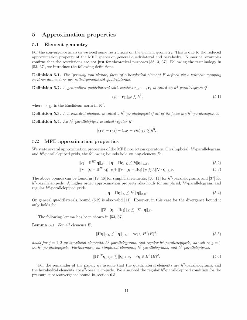
T , i = 1, . . . , 8, the eight corresponding vertices of element E as shown in Figure 1. We notethat the element can have non-planar faces. The outward unit normal vectors to the faces of E and E aredenoted by ni and ni, i = 1, . . . , 6, respectively. In this case FE is a trilinear mapping given by

FE(r) = r1(1 − x)(1 − y)(1 − z) + r2x(1 − y)(1 − z) + r3xy(1 − z) + r4(1 − x)y(1 − z)

+ r5(1 − x)(1 − y)z + r6x(1 − y)z + r7xyz + r8(1 − x)yz

= r1 + r21x+ r41y + r51z + (r34 − r21)xy + (r65 − r21)xz + (r85 − r41)yz

+ (r21 − r34 − r65 + r78)xyz,

(3.1)

4

r1 r2

r3

r4

r5 r6

r7r8

FE

r1 r2

r3

r4

r5r6

r7r8

E

n2

n1

n2

E

n1

Figure 1: Trilinear hexahedral mapping.

where rij = ri−rj . It is easy to see that each component of DFE is a bilinear function of two space variables:

DFE(r) = [r21 + (r34 − r21)y + (r65 − r21)z + (r21 − r34 − r65 + r78)yz,

r41 + (r34 − r21)x+ (r85 − r41)z + (r21 − r34 − r65 + r78)xz,

r51 + (r65 − r21)x+ (r85 − r41)y + (r21 − r34 − r65 + r78)xy].

(3.2)

In the case of tetrahedra, E is the reference tetrahedron with vertices r1 = (0, 0, 0)T , r2 = (1, 0, 0)T ,r3 = (0, 1, 0)T , and r4 = (0, 0, 1)T . Let ri, i = 1, . . . , 4, be the corresponding vertices of E. The linearmapping for tetrahedra has the form

FE(r) = r1(1 − x− y − z) + r2x+ r3y + r4z (3.3)

with respective Jacobian matrix and its determinant

DFE = [r21, r31, r41] and JE = 2|E|, (3.4)

where |E| is the area of element E.The mappings in the cases of quadrilaterals and triangles are described similarly to the cases of hexahedra

and tetrahedra, respectively. Note that in the case of simplicial elements the mapping is affine and theJacobian matrix and its determinant are constants. This is not the case for quadrilaterals and hexahedra.

In all above elements JE(r) is uniformly positive, since E is convex. Using the above mapping definitions

and the classical formula ∇φ = (DFE)−1∇φ, for φ(r) = φ(r), it is easy to see that for any face or edgeei ⊂ E,

ni =DF−T

E ni

|DF−TE ni|

. (3.5)

Also, the shape regularity and quasi-uniformity of the grids imply that for all elements E ∈ Th,

‖DFE‖0,∞,E . h, ‖JE‖0,∞,E h hd, ‖DF−1E ‖0,∞,E . h−1, ‖JF−1

E‖0,∞,E h h−d. (3.6)

3.2 Mixed finite element spaces

We introduce four finite element spaces with respect to the four types of elements considered in this paper.Let V(E) and W (E) denote the finite element spaces on the reference element E.

For simplicial elements, we employ BDM1 [18] on triangles and BDDF1 [17] on tetrahedra:

V(E) = (P1(E))d, W (E) = P0(E), (3.7)

where Pk denotes the space of polynomials of degree ≤ k.

5

On the unit square, we employ BDM1 [18]:

V(E) = (P1(E))2 + r curl(x2y) + s curl(xy2), W (E) = P0(E), (3.8)

where r and s are real constants.On the unit cube, we employ the enhanced BDDF1 space [37]:

V(E) = BDDF1(E) + r2curl(0, 0, x2z)T + r3curl(0, 0, x2yz)T + s2curl(xy2, 0, 0)T

+ s3curl(xy2z, 0, 0)T + t2curl(0, yz2, 0)T + t3curl(0, xyz2, 0)T ,

W (E) = P0(E),

(3.9)

where the BDDF1 space on unit cube [17] is defined as

BDDF1(E) = (P1(E))3 + r0curl(0, 0, xyz)T + r1curl(0, 0, xy2)T + s0curl(xyz, 0, 0)T

+ s1curl(yz2, 0, 0)T + t0curl(0, xyz, 0)T + t1curl(0, x2z, 0)T ,

where ri, si, ti, i = 0, . . . 3, are real constants.Note that in all four cases

∇ · V(E) = W (E). (3.10)

On any face (edge in 2D) e ∈ E, for all v ∈ V (E), v · ne ∈ P1(e) on the reference square or simplex, andv · ne ∈ Q1(e) on the reference cube, where Q1(e) is the space of bilinear functions on e.

The degrees of freedom for V(E) are chosen to be the values of v · ne at the vertices of e, for each face(edge) e. This choice gives certain orthogonalities for the quadrature rule introduced in the next section andleads to a cell-centered pressure scheme.

The spaces V(E) and W (E) on any physical element E ∈ Th are defined, respectively, via the Piolatransformation

v ↔ v : v =1

JEDFEv F−1

E

and standard scalar transformationw ↔ w : w = w F−1

E .

Under these transformations, the divergence and the normal components of the velocity vectors on the faces(edges) are preserved [19]:

(∇ · v, w)E = (∇ · v, w)E and 〈v · ne, w〉e = 〈v · ne, w〉e. (3.11)

In addition, (3.5) implies that

v · ne =1

|JEDF−TE ne|

v · ne, (3.12)

and (3.11) implies that

∇ · v =

(1

JE∇ · v

) F−1

E (x). (3.13)

On quadrilaterals or hexahedra, ∇ · v 6= constant since JE is not constant.The finite element spaces Vh,i and Wh,i on subdomain Ωi are given by

Vh,i =v ∈ V : v|E ↔ v, v ∈ V(E), ∀E ∈ Th,i

,

Wh,i =w ∈W : w|E ↔ w, w ∈ W (E), ∀E ∈ Th,i

.

(3.14)

6

The global mixed finite element spaces are defined as

Vh =

n⊕

i=1

Vh,i, Wh =

n⊕

i=1

Wh,i.

We recall the projection operator in the space Vh,i. The operator Π : (H1(E))d → V(E) is defined locallyon each element by

〈(Πq− q) · ne, q1〉e = 0, ∀e ⊂ ∂E, (3.15)

where q1 ∈ P1(e) when E the unit square or simplicial element, and q1 ∈ Q1(e) when E is the unit cube.The global operator Π : V ∩ (H1(Ω))d → Vh on each element E is defined via the Piola transformation:

Πq ↔ Πq, Πq = Πq. (3.16)

Furthermore, (3.11), (3.15), and (3.16) imply that Πq ·n is continuous across element interfaces, which givesΠq ∈ Vh,i, and that

(∇ · (Πq − q), w)Ωi= 0, ∀w ∈Wh,i. (3.17)

In the analysis, we also need similar projection operators onto the lowest order Raviart-Thomas [45, 44].The RT0 spaces are defined on the reference cube and the reference tetrahedron, respectively, as

VRT (E) =

r1 + s1xr2 + s2yr3 + s3z

, WRT (E) = P0(E), (3.18)

and

VRT (E) =

r1 + sxr2 + syr3 + sz

, WRT (E) = P0(E), (3.19)

with similar definitions in two dimensions, where s, ri, si (i=1,2,3) are constants.

In all cases ∇·VRT = WRT (E) and v·ne ∈ P0(e). The degrees of freedom of VRT (E) are chosen to be the

values of v·ne at the midpoints of all faces (edges) of E. The projection operator ΠRT : (H1(E))d → VRT (E)satisfies

〈(ΠRT q − q) · ne, q0〉e = 0, ∀e ⊂ ∂E, ∀q0 ∈ P0(E). (3.20)

The spaces VRTh and WRT

h on Ω and the projection operator ΠRT : (H1(Ω))d → VRTh are defined similarly

to the case of Vh and Wh. By definition, we have

VRTh,i ⊂ Vh,i WRT

h,i = Wh,i. (3.21)

The projection operator ΠRT satisfies

(∇ · (ΠRT q − q), w) = 0, ∀w ∈ WRTh,i , (3.22)

∇ · ΠRT v = ∇ · v, ∀v ∈ Vh,i, (3.23)

and for all element E ∈ Th,i,‖ΠRTv‖E . ‖v‖E , ∀v ∈ Vh,i. (3.24)

Furthermore, due to (3.15) and (3.20),ΠRT Πq = ΠRT q. (3.25)

7

3.3 A quadrature rule

Recall the variational formulation (2.3)–(2.4). In its mixed finite element discretization, one needs to computethe integral (K−1q,v)Ωi

for q,v ∈ Vh,i. The MFMFE method employs a quadrature rule for the velocitymass matrix, in order to reduce the discrete problem on each subdomain to a cell-centered finite differencesystem for the pressure. We follow the development in [53, 37]. The integration on each element E isperformed by mapping to the reference element E, where the quadrature rule is defined. Using the definition(3.14) of the finite element spaces, for q,v ∈ Vh,i,

(K−1q,v)E =

(1

JEDFT

EK−1(FE(x))DFE q, v

)

E

≡ (K−1q, v)E ,

where

K−1(x) =1

JEDFT

EK−1(FE(x))DFE . (3.26)

Due to (3.6), we have‖K−1‖0,∞,E h h2−d‖K−1‖0,∞,E. (3.27)

The quadrature rule on an element E is defined by the trapezoidal rule:

(K−1q,v)Q,E = (K−1q, v)Q,E ≡|E|

nv

nv∑

i=1

K−1(ri)q(ri) · v(ri), (3.28)

where nv is the number of vertices of E. The global quadrature rule on Ωi is defined as

(K−1q,v)Q,Ωi≡

∑

E∈Th,i

(K−1q,v)Q,E .

The corner vector q(ri) is uniquely determined by its normal components to the d faces that share thevertex. Since we chose the velocity degrees freedom associated with each corner ri, the d degrees of freedomassociated with each corner ri uniquely determine the corner vector q(ri). More precisely,

q(ri) =

d∑

j=1

(q · nij)(ri)nij ,

where nij , j = 1, . . . , d, are the outward unit normal vectors to the d faces (or edges) sharing ri, and(q · nij)(ri) are the velocity degrees of freedom associated with this corner. Denote the basis functionsassociated with ri by vij , j = 1, . . . , d:

(vij · nij)(ri) = 1, (vij · nik)(ri) = 0, k 6= j, and (vij · nlk)(rl) = 0, l 6= i, k = 1, . . . , d.

The quadrature rule (3.28) couples only the d basis functions associated with a corner. For example, on theunit cube,

(K−1v11, v11)Q,E =K−1

11 (r1)

8, (K−1v11, v12)Q,E =

K−121 (r1)

8,

(K−1v11, v13)Q,E =K−1

31 (r1)

8, and (K−1v11, vij)Q,E = 0 i 6= 1, j = 1, 2, 3.

(3.29)

Mapping back to the physical element E, we have

(K−1q,v)Q,E =1

nv

nv∑

i=1

JE(ri)K−1(ri)q(ri) · v(ri), (3.30)

8

which is closely related to an inner products used in the mimetic finite difference methods [36].It has been shown [53, 37] that the bilinear form (K−1q,v)Q,Ωi

is an inner product in Vh,i and

(K−1q,q)1/2Q,Ωi

is a norm equivalent to ‖ · ‖Ωi:

(K−1q,q)Q,Ωih ‖q‖2

Ωi∀q ∈ Vh,i. (3.31)

In the pressure superconvergence analysis, we need additional property of the bilinear form (K−1·, ·)Q,Ωion

the space

Vh,i := Vh,i

⋃Wh,i,

where Wh,i is the space of piecewise constant vectors defined element by element.

Lemma 3.1. The bilinear form (K−1·, ·)Q,Ωiis an inner product on Vh,i and the norm (K−1q,q)

1/2Q,Ωi

on

Vh,i is equivalent to ‖ · ‖Ωi:

(K−1q,q)1/2Q,Ωi

h ‖q‖Ωi, ∀q ∈ Vh,i. (3.32)

Proof. On each element E, let q =∑nv

i=1

∑dj=1 qijvij + q0 where vij are the normalized basis functions of

Vh,i(E) and q0 is a constant vector. Using (3.30), (1.4), (3.6), we have

(K−1q,q)Q,E &|E|

k1

nv∑

i=1

d∑

j=1

q2ij + |q0|2

.

This gives that (K−1·, ·)Q,E is an inner product. Using (3.27), the fact that ‖q‖2E h h2−d‖q‖2

Efor all

q ∈ (L2(E))d (see Lemma 2.3 in [53]), and norm equivalence on the reference element E, we obtain for allq ∈ Vh,

(K−1q,q)Q,E = (K−1q, q)Q,E h h2−d‖q‖2E

h ‖q‖2E .

The numerical quadrature error on each element is defined as

σE(q,v) ≡ (q,v)E − (q,v)Q,E , (3.33)

and the global numerical quadrature error is given by σ(q,v)|E ≡ σE(q,v).

3.4 Reduction to a cell centered finite difference system for the pressure

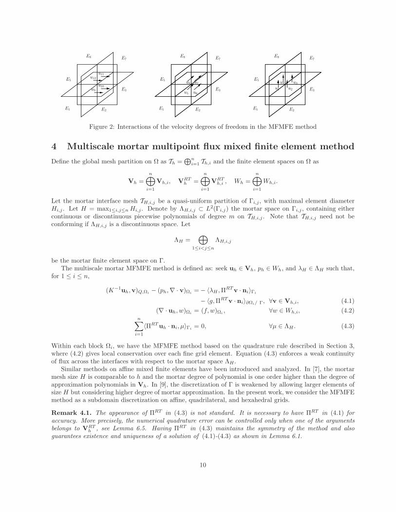
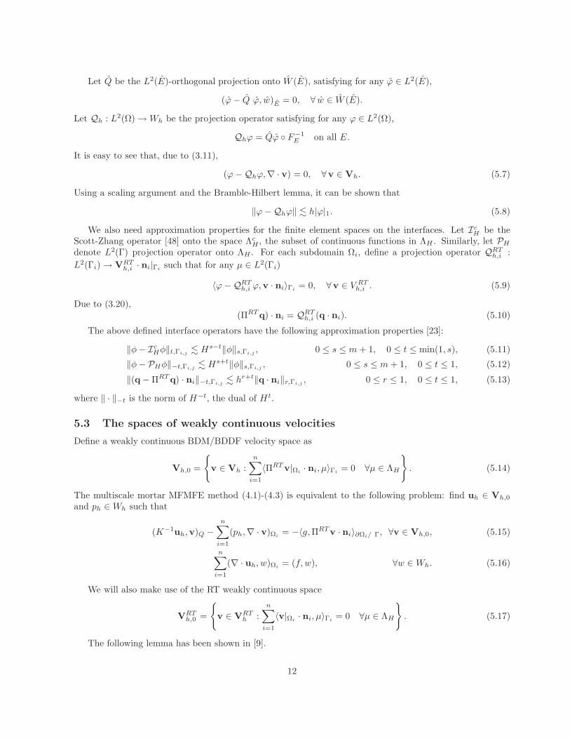
We next describe how the quadrature rule for the velocity mass matrix allows one to reduce the MFMFEmethod on each subdomain to a centered finite difference system for the pressure. We limit the discussionto hexahedral grids; the other element types are treated similarly. We refer to Figure 2 for the notation usedin this section. Any interior vertex r is shared by 8 elements E1, . . . , E8. We denote the faces that share thevertex by e1, . . . , e12, and the velocity basis functions on these faces that are associated with the vertex byv1, . . . ,v12, i.e., (vi · ni)(r) = 1, where ni is the unit normal on face ei. The corresponding values of thenormal components of uh, u1, . . . , u12 are depicted in the three images in directions x, y, and z, respectively.

Recall that the quadrature rule (K−1·, ·)Q localizes the basis functions interaction, see (3.29). Therefore,taking v = v1 in (4.1), for example, will lead to coupling u1 only with u5, u8, u9, and u12. Similarly,u2 will be coupled only with u6, u7, u9, and u12, etc. Therefore, the 12 equations obtained from takingv = v1, . . . ,v12 form a linear system for u1, . . . , u12. The following result is a direct consequence of (3.31).

Proposition 3.1. The 12 × 12 local linear system described above is symmetric and positive definite.

The solution of the local 12×12 linear system allows for the velocities ui, i = 1, . . . , 12 to be expressed interms of the cell-centered pressures pi, i = 1, . . . , 8. Substituting these expressions into the mass conservationequation (4.2) leads to a cell-centered stencil. The pressure in each element E is coupled with the pressuresin the elements that share a vertex with E, leading to a 27 point stencil. The reader is referred to [53, 37]for further details on the resulting cell-centered finite difference system.

9

E3

E7E8

E5

E2E1

u12

u9

u10

u11

E3

E7E8

E5

E2E1

u5 u6

u7u8

E3

E7E8

E5

E2E1

u1 u2

u3u4

Figure 2: Interactions of the velocity degrees of freedom in the MFMFE method

4 Multiscale mortar multipoint flux mixed finite element method

Define the global mesh partition on Ω as Th =⊕n

i=1 Th,i and the finite element spaces on Ω as

Vh =n⊕

i=1

Vh,i, VRTh =

n⊕

i=1

VRTh,i , Wh =

n⊕

i=1

Wh,i.

Let the mortar interface mesh TH,i,j be a quasi-uniform partition of Γi,j , with maximal element diameterHi,j . Let H = max1≤i,j≤n Hi,j . Denote by ΛH,i,j ⊂ L2(Γi,j) the mortar space on Γi,j , containing eithercontinuous or discontinuous piecewise polynomials of degree m on TH,i,j . Note that TH,i,j need not beconforming if ΛH,i,j is a discontinuous space. Let

ΛH =⊕

1≤i<j≤n

ΛH,i,j

be the mortar finite element space on Γ.The multiscale mortar MFMFE method is defined as: seek uh ∈ Vh, ph ∈Wh, and λH ∈ ΛH such that,

for 1 ≤ i ≤ n,

(K−1uh,v)Q,Ωi− (ph,∇ · v)Ωi

= − 〈λH ,ΠRTv · ni〉Γi

− 〈g,ΠRT v · ni〉∂Ωi/ Γ, ∀v ∈ Vh,i, (4.1)

(∇ · uh, w)Ωi= (f, w)Ωi

, ∀w ∈ Wh,i, (4.2)n∑

i=1

〈ΠRT uh · ni, µ〉Γi= 0, ∀µ ∈ ΛH . (4.3)

Within each block Ωi, we have the MFMFE method based on the quadrature rule described in Section 3,where (4.2) gives local conservation over each fine grid element. Equation (4.3) enforces a weak continuityof flux across the interfaces with respect to the mortar space ΛH .

Similar methods on affine mixed finite elements have been introduced and analyzed. In [7], the mortarmesh size H is comparable to h and the mortar degree of polynomial is one order higher than the degree ofapproximation polynomials in Vh. In [9], the discretization of Γ is weakened by allowing larger elements ofsize H but considering higher degree of mortar approximation. In the present work, we consider the MFMFEmethod as a subdomain discretization on affine, quadrilateral, and hexahedral grids.

Remark 4.1. The appearance of ΠRT in (4.3) is not standard. It is necessary to have ΠRT in (4.1) foraccuracy. More precisely, the numerical quadrature error can be controlled only when one of the argumentsbelongs to VRT

h , see Lemma 6.5. Having ΠRT in (4.3) maintains the symmetry of the method and alsoguarantees existence and uniqueness of a solution of (4.1)-(4.3) as shown in Lemma 6.1.

10

5 Approximation properties

5.1 Element geometry

For the convergence analysis we need some restrictions on the element geometry. This is due to the reducedapproximation property of the MFE spaces on general quadrilateral and hexahedra. Numerical examplesconfirm that the restrictions are not just for theoretical purposes [53, 3, 37]. Following the terminology in[53, 37], we introduce the following definitions.

Definition 5.1. The (possibly non-planar) faces of a hexahedral element E defined via a trilinear mappingin three dimensions are called generalized quadrilaterals.

Definition 5.2. A generalized quadrilateral with vertices r1, · · · , r4 is called an h2-parallelogram if

|r34 − r21|Rd . h2, (5.1)

where | · |Rd is the Euclidean norm in Rd.

Definition 5.3. A hexahedral element is called a h2-parallelepiped if all of its faces are h2-parallelograms.

Definition 5.4. An h2-parallelepiped is called regular if

|(r21 − r34) − (r65 − r78)|Rd . h3.

5.2 MFE approximation properties

We state several approximation properties of the MFE projection operators. On simplicial, h2-parallelogram,and h2-parallelepiped grids, the following bounds hold on any element E:

‖q− ΠRT q‖E + ‖q− Πq‖E . h‖q‖1,E, (5.2)

‖∇ · (q − ΠRT q)‖E + ‖∇ · (q − Πq)‖E . h‖∇ · q‖1,E . (5.3)

The above bounds can be found in [19, 46] for simplicial elements, [50, 11] for h2-parallelograms, and [37] forh2-parallelepipeds. A higher order approximation property also holds for simplicial, h2-parallelogram, andregular h2-parallelepiped grids:

‖q− Πq‖E . h2‖q‖2,E. (5.4)

On general quadrilaterals, bound (5.2) is also valid [11]. However, in this case for the divergence bound itonly holds for

‖∇ · (q − Πq)‖E . ‖∇ · q‖E .

The following lemma has been shown in [53, 37].

Lemma 5.1. For all elements E,

‖Πq‖j,E . ‖q‖j,E , ∀q ∈ Hj(E)d, (5.5)

holds for j = 1, 2 on simplicial elements, h2-parallelograms, and regular h2-parallelepipeds, as well as j = 1on h2-parallelepipeds. Furthermore, on simplicial elements, h2-parallelograms, and h2-parallelepipeds,

‖ΠRT q‖1,E . ‖q‖1,E , ∀q ∈ H1(E)d. (5.6)

For the remainder of the paper, we assume that the quadrilateral elements are h2-parallelograms, andthe hexahedral elements are h2-parallelepipeds. We also need the regular h2-parallelepiped condition for thepressure superconvergence bound in section 6.5.

11

Let Q be the L2(E)-orthogonal projection onto W (E), satisfying for any ϕ ∈ L2(E),

(ϕ− Q ϕ, w)E = 0, ∀ w ∈ W (E).

Let Qh : L2(Ω) →Wh be the projection operator satisfying for any ϕ ∈ L2(Ω),

Qhϕ = Qϕ F−1E on all E.

It is easy to see that, due to (3.11),

(ϕ−Qhϕ,∇ · v) = 0, ∀v ∈ Vh. (5.7)

Using a scaling argument and the Bramble-Hilbert lemma, it can be shown that

‖ϕ−Qhϕ‖ . h|ϕ|1. (5.8)

We also need approximation properties for the finite element spaces on the interfaces. Let IcH be the

Scott-Zhang operator [48] onto the space ΛcH , the subset of continuous functions in ΛH . Similarly, let PH

denote L2(Γ) projection operator onto ΛH . For each subdomain Ωi, define a projection operator QRTh,i :

L2(Γi) → VRTh,i · ni|Γi

such that for any µ ∈ L2(Γi)

〈ϕ−QRTh,i ϕ,v · ni〉Γi

= 0, ∀v ∈ V RTh,i . (5.9)

Due to (3.20),(ΠRT q) · ni = QRT

h,i (q · ni). (5.10)

The above defined interface operators have the following approximation properties [23]:

‖φ− IcHφ‖t,Γi,j

. Hs−t‖φ‖s,Γi,j, 0 ≤ s ≤ m+ 1, 0 ≤ t ≤ min(1, s), (5.11)

‖φ− PHφ‖−t,Γi,j. Hs+t‖φ‖s,Γi,j

, 0 ≤ s ≤ m+ 1, 0 ≤ t ≤ 1, (5.12)

‖(q− ΠRT q) · ni‖−t,Γi,j. hr+t‖q · ni‖r,Γi,j

, 0 ≤ r ≤ 1, 0 ≤ t ≤ 1, (5.13)

where ‖ · ‖−t is the norm of H−t, the dual of Ht.

5.3 The spaces of weakly continuous velocities

Define a weakly continuous BDM/BDDF velocity space as

Vh,0 =

v ∈ Vh :

n∑

i=1

〈ΠRT v|Ωi· ni, µ〉Γi

= 0 ∀µ ∈ ΛH

. (5.14)

The multiscale mortar MFMFE method (4.1)-(4.3) is equivalent to the following problem: find uh ∈ Vh,0

and ph ∈ Wh such that

(K−1uh,v)Q −n∑

i=1

(ph,∇ · v)Ωi= −〈g,ΠRTv · ni〉∂Ωi/ Γ, ∀v ∈ Vh,0, (5.15)

n∑

i=1

(∇ · uh, w)Ωi= (f, w), ∀w ∈ Wh. (5.16)

We will also make use of the RT weakly continuous space

VRTh,0 =

v ∈ VRT

h :

n∑

i=1

〈v|Ωi· ni, µ〉Γi

= 0 ∀µ ∈ ΛH

. (5.17)

The following lemma has been shown in [9].

12

Lemma 5.2. Under assumption (5.24), there exists a projection operator ΠRT0 :

(H1/2+ǫ(Ω)

)d∩V → VRT

h,0

such that

(∇ · (ΠRT0 q − q), w)Ωi

= 0, w ∈Wh, 1 ≤ i ≤ n, (5.18)

‖ΠRT0 q − ΠRT q‖ . ‖q‖r+1/2h

rH1/2, 0 < r ≤ 1, (5.19)

‖ΠRT0 q − q‖ .

n∑

i=1

‖q‖1,Ωih+ ‖q‖r+1/2h

rH1/2, 0 < r ≤ 1. (5.20)

In the following we construct a projection operator Π0 into Vh,0 with similar properties.By an abuse of notation, define

VRTh,0 · n =(φL, φR) ∈ L2(Γ) × L2(Γ) : ∃v ∈ VRT

h,0 such that

φL|Γi,j= v|Ωi

· ni and φR|Γi,j= v|Ωj

· nj ∀1 ≤ i < j ≤ n.

Then, for any φ = (φL, φR) ∈ (L2(Γ))2, we write φ|Γi,j= (φi, φj), 1 ≤ i < j ≤ n. Define a projection

operator QRTh,0 : (L2(Γ))2 → VRT

h,0 · n such that, for any φ ∈ (L2(Γ))2,

n∑

i=1

〈φi − (QRTh,0φ)i, ηi〉Γi

= 0, ∀ η ∈ VRTh,0 · n. (5.21)

The proof of the following two lemmas can be found in [7, Section 3], with a straightforward modificationof the argument for the two scales h and H .

Lemma 5.3. Assume that for any µ ∈ ΛH ,

QRTh,i µ = 0, 1 ≤ i ≤ n, implies that µ = 0. (5.22)

Then, for any φ ∈ (L2(Γ))2, there exists λH ∈ ΛH such that on Γi,j , 1 ≤ i ≤ j ≤ n,

QRTh,i λH = QRT

h,i φi − (QRTh,0φ)i, QRT

h,j λH = QRTh,j φj − (QRT

h,0φ)j , and 〈λH , 1〉Γi,j=

1

2〈φi + φj , 1〉Γi,j

.

(5.23)

Lemma 5.4. Assume that for any µ ∈ ΛH ,

‖µ‖Γi,j≤ C

(‖QRT

h,i µ‖Γi,j+ ‖QRT

h,j µ‖Γi,j

), 1 ≤ i < j ≤ n. (5.24)

Then, for any φ|Γi,j= (φi,−φi),

∑

1≤i<j≤n

‖QRTh,i φi − (QRT

h,0φ)i‖2−s,Γi,j

1/2

.∑

1≤i<j≤n

‖φi‖r,Γi,jhrHs, 0 ≤ r ≤ 1, 0 ≤ s ≤ 1. (5.25)

We are now ready to construct a projection operator Π0 onto Vh,0. Our approach is similar to the onein [7]. For any q ∈ (H1/2+ǫ(Ω))d ∩ V, ǫ > 0, define

Π0q|Ωi= Π(q + δqi),

where δqi solves

δqi = −∇πi in Ωi, (5.26)

∇ · δqi = 0 in Ωi, (5.27)

δqi · ni = −QRTh,i q · ni + (QRT

h,0q · n)i on Γi, (5.28)

δqi · ni = 0 on ∂Ωi ∩ ∂Ω, (5.29)

13

where q · n|Γi,j= (q · ni,q · nj). The Neumann problem (5.26)-(5.29) is solvable, since (5.23) imply the

solvability condition〈QRT

h,i q · ni − (QRTh,0q · n)i, 1〉Γi

= 0.

By the construction of Π0 and using (3.25), for all µ ∈ ΛH ,

n∑

i=1

〈ΠRT (Π0q) · ni, µ〉Γi=

n∑

i=1

〈ΠRT (q + δqi) · ni, µ〉Γi

=

n∑

i=1

〈QRTh,i (q + δqi) · ni, µ〉Γi

=

n∑

i=1

〈(QRTh,0q · n)i, µ〉Γi

= 0,

where we have used (5.10) and (5.28). Thus, Π0q ∈ Vh,0. Also,

(∇ · Π0q, w)Ωi= (∇ · Πq, w)Ωi

+ (∇ · Πδqi, w)Ωi= (∇ · q, w)Ωi

, ∀w ∈Wh,i.

It remains to estimate the approximability of Π0. Since Π0q − Πq = Πδqi, we only need to bound thecorrection term Πδqi. By elliptic regularity [33, 41], for any 0 ≤ s ≤ 1/2,

‖δqi‖1/2−s,Ωi.

∑

j

‖QRTh,i q · ni − (QRT

h,0q · n)i‖−s,Γi,j. (5.30)

Then we have

‖Πδqi‖Ωi≤ ‖Πδqi − δqi‖Ωi

+ ‖δqi‖Ωi. h1/2‖δqi‖1/2,Ωi

+ ‖δqi‖Ωi

.∑

j

(h1/2‖QRTh,i q · ni − (QRT

h,0q · n)i‖Γi,j+ ‖QRT

h,i q · ni − (QRTh,0q · n)i‖−1/2,Γi,j

), (5.31)

where we have used an estimate for any divergence-free vector ψ [43]

‖Πψ −ψ‖Ωi. hr‖ψ‖r,Ωi

, 0 < r ≤ 1. (5.32)

Note that the above result was shown in [43] for the Raviart-Thomas spaces, but it can be easily extendedto the other mixed finite element spaces under consideration. Applying Lemma 5.4 and the trace theorem(see Theorem 1.5.2.1 in [33]):

‖q‖r,Γi,j. ‖q‖r+1/2,Ωi

, r > 0, (5.33)

(5.31) yields the following result.

Lemma 5.5. Under assumption (5.24), there exists a projection operator Π0 :(H1/2+ǫ(Ω)

)d∩ V → Vh,0

such that

(∇ · (Π0q − q), w)Ωi= 0, w ∈ Wh, 1 ≤ i ≤ n, (5.34)

‖Π0q − Πq‖ . ‖q‖r+1/2hrH1/2, 0 < r ≤ 1, (5.35)

‖Π0q − q‖ .

n∑

i=1

‖q‖1,Ωih+ ‖q‖r+1/2h

rH1/2, 0 < r ≤ 1, (5.36)

Inequality (5.36) is a direct consequence of (5.35) and (5.2).In the next Lemma we establish some continuity properties for Π0 and ΠRT

0 .

Lemma 5.6. Under assumption (5.24), on simplicial, quadrilaterals, and hexahedral elements,

‖Π0q‖ + ‖ΠRT0 q‖ .

n∑

i=1

‖q‖1,Ωi+ ‖q‖r+1/2, 0 < r ≤ 1, (5.37)

14

∑

E∈Th

(‖Π0q‖1,E + ‖ΠRT0 q‖1,E) .

n∑

i=1

‖q‖1,Ωi+ hr−1H1/2‖q‖r+1/2, 0 < r ≤ 1, (5.38)

∀E ∈ Th, ‖∇ · Π0q‖E + ‖∇ · ΠRT0 q‖E . ‖∇ · q‖E . (5.39)

Proof. We present the proof for Π0. The proof for ΠRT0 is similar. Bound (5.37) for Π0 follows from the

triangle inequality ‖Π0q‖ ≤ ‖q − Π0q‖ + ‖q‖ and (5.36).For (5.38), we use the triangle and inverse inequality:

∑

E∈Th

‖Π0q‖1,E .∑

E∈Th

(‖Π0q − Πq‖1,E + ‖Πq‖1,E) .∑

E∈Th

(h−1‖Π0q − Πq‖E + ‖Πq‖1,E

).

Bound (5.38) follows by combining the above inequality with (5.35) and (5.5).To show (5.39), we first note that if v ∈ Vh and (∇ · v, w) = 0 ∀w ∈ Wh, then ∇ · v = 0. This follows

from (3.11), and (3.10). Now the definition of Π0 implies that ∇ · Π0q = ∇ · Πq. Furthermore, using (3.13)and (3.6),

‖∇ · Πq‖E . h−d/2E ‖∇ · Πq‖E ≤ h

−d/2E ‖∇ · q‖E . ‖∇ · q‖E ,

where we have used that ∇ · Πq is the L2(E)-projection of ∇ · q. This completes the proof of (5.39).

In the convergence analysis below we will need the trace inequality (see [31])

〈q,v · n〉∂Ωi. ‖q‖1/2,∂Ωi

‖v‖H(div;Ωi), (5.40)

and the following lemma.

Lemma 5.7. For all v ∈ VRTh,i ,

‖v · ni‖∂E h h−1/2‖v‖E . (5.41)

Proof. The result follows from the scaling estimate [53]: ‖v‖E h h(2−d)/2‖v‖E , the norm equivalence on the

reference element E : ‖v · ni‖∂E h ‖v‖E, and (3.12).

6 Convergence analysis

6.1 Solvability

The next lemma shows the solvability of the multiscale mortar MFMFE method.

Lemma 6.1. Assume that (5.22) holds. Then, there exists a unique solution of (4.1)-(4.3).

Proof. It is sufficient to show the uniqueness since (4.1)-(4.3) is a finite-dimensional linear square system.Let f = 0 and g = 0. Choosing v = uh, w = ph, and µ = λH , adding (4.1)-(4.3) together, and summingover 1 ≤ i ≤ n implies that

n∑

i=1

(K−1uh,uh)Q,Ωi= 0.

The norm equivalence (3.31) implies that uh = 0. Given ph ∈ Wh ⊂ L2(Ω), there exists q ∈ (H1(Ω))d suchthat ∇ · q = ph. Such vector field can be easily constructed by solving

∆φ = ph in B, φ = 0 on ∂B, (6.1)

where B is an open ball containing Ω and ph is the extension of ph by zero on B, and taking q = ∇φ.By elliptic regularity [41], φ ∈ H2(B) and therefore q ∈ (H1(Ω))d, satisfying ‖q‖1 . ‖ph‖. The aboveconstruction is possible since no boundary conditions on ∂Ω are imposed on the velocity field. We note that

15

a vector field q with the required properties can also be constructed for a Lipschitz domain Ω when fluxboundary conditions are imposed on (part of) ∂Ω [31, 29].

Take v = Π0q in (4.1) to get 0 =∑n

i=1(ph,∇ ·Π0q) = (ph,∇ · q) = ‖ph‖2, implying ph = 0. Then, (4.1)gives 0 = 〈λH ,Π

RT v · ni〉Γi= 〈QRT

h,i λH ,ΠRTv · ni〉Γi

for all v ∈ Vh. Also, there exists v ∈ VRTh such that

v · ni = QRTh,i λH , implying QRT

h,i λH = 0 and, due to (5.22), λH = 0.

6.2 Optimal convergence estimate for the velocity

In this section we derive a priori error estimates for the velocity. Subtracting (5.15)-(5.16) from (2.3)-(2.4)gives the error equations

(K−1u,v

)−

(K−1uh,v

)Q

=

n∑

i=1

(p− ph,∇ · v)Ωi−

n∑

i=1

〈p,v · ni〉Γi

−n∑

i=1

〈g, (v − ΠRT v) · ni〉∂Ωi/Γ, ∀v ∈ Vh,0, (6.2)

n∑

i=1

(∇ · (u− uh), w)Ωi= 0, ∀w ∈ Wh, (6.3)

For the permeability tensor K, we will use the following notation. Let W k,∞Th

consist of functions φ such

that φ|E ∈W k,∞(E) for all E ∈ Th and ‖φ‖k,∞,E is uniformly bounded. Let |||φ|||k,∞ = maxE∈Th‖φ‖k,∞,E .

The following two lemmas give bounds on terms that appear in the velocity error analysis.

Lemma 6.2 ([53, 37]). On simplicial elements, h2-parallelograms, and h2-parallelepipeds, if K−1 ∈ W 1,∞Th

,then for all v ∈ Vh,

|(K−1Πu,v − ΠRT v)Q| .

n∑

i=1

h|||K−1|||1,∞‖u‖1,Ωi‖v‖Ωi

. (6.4)

Lemma 6.3 ([53, 37]). On simplicial elements, h2-parallelograms, and h2-parallelepipeds, if K−1 ∈ W 1,∞Th

,

then for all q ∈ Vh and for all v ∈ VRTh ,

|σ(K−1q,v)| .∑

E∈Th

h‖K−1‖1,∞,E‖q‖1,E‖v‖0,E . (6.5)

We are now ready to establish the main a priori velocity bound.

Theorem 6.1. Let K−1 ∈ W 1,∞Th

. For the velocity uh of the mortar MFMFE method (4.1)-(4.3) on simplicial

elements, h2-parallelograms, and h2-parallelepipeds, if (5.24) holds, then

n∑

i=1

‖∇ · (u − uh)‖Ωi.

n∑

i=1

h‖∇ · u‖1,Ωi, (6.6)

‖u− uh‖ .

n∑

i=1

(Hs−1/2‖p‖s+1/2,Ωi+ h‖u‖1,Ωi

) + hrH1/2‖u‖r+1/2, (6.7)

where 1/2 ≤ s ≤ m+ 1, 0 < r ≤ 1.

Proof. First we note that

∇ · (Πu − uh) = 0 and ∇ · (Π0u− uh) = 0 in Ωi, i = 1, . . . , n, (6.8)

which follow from (6.3), (3.17), (5.34), (3.11), and (3.10). The divergence error bound (6.6) now follows from(5.3).

16

For all v ∈ Vh,0 such that ∇ · v = 0 in each subdomain, the error equation (6.2) gives

(K−1u,v

)−

(K−1uh,v

)Q

= −n∑

i=1

〈p, (v − ΠRT v) · ni〉Γi

−n∑

i=1

〈p− IcHp,Π

RT v · ni〉Γi−

n∑

i=1

〈g, (v − ΠRT v) · ni〉∂Ωi/Γ,

where we have used thatn∑

i=1

〈IcHp,Π

RTv · ni〉Γi= 0. (6.9)

Taking v − ΠRT v ∈ Vh as a test function in (2.3) gives

(K−1u,v − ΠRT v) = −n∑

i=1

〈g, (v − ΠRT v) · ni〉∂Ωi/Γ −n∑

i=1

〈p, (v − ΠRT v) · ni〉Γi.

The above two equations imply

(K−1uh,v

)Q

=(K−1u,ΠRT v

)+

n∑

i=1

〈p− IcHp,Π

RT v · ni〉Γi∀v ∈ Vh,0 s.t. ∇ · v = 0. (6.10)

By using (6.10), we rewrite(K−1(Π0u− uh),v

)Q

as

(K−1(Π0u − uh),v)Q =(K−1Π0u,v

)Q−

(K−1u,ΠRT v

)−

n∑

i=1

〈p− IcHp,Π

RT v · ni〉Γi

=(K−1(Π0u− Πu),v

)Q

+(K−1Πu,v − ΠRT v

)Q− σ

(K−1Πu,ΠRT v

)

+(K−1(Πu − u),ΠRT v

)−

n∑

i=1

〈p− IcHp,Π

RTv · ni〉Γi.

(6.11)

The first and fourth terms on the right hand side of (6.11) can be estimated by using (5.35) and (5.2),respectively: (

K−1(Π0u − Πu),v)

Q. hrH1/2‖u‖r+1/2‖v‖, 0 < r ≤ 1, (6.12)

(K−1(Πu − u),ΠRT v

).

n∑

i=1

h‖u‖1,Ωi‖v‖Ωi

, (6.13)

where we have also used (3.24). Using (6.5), (3.24), and (5.5), we bound the third term on the right in (6.11)as

|σ(K−1Πu,ΠRT v)| .∑

E∈Th

h‖Πu‖1,E‖ΠRTv‖E .

n∑

i=1

h‖u‖1,Ωi‖v‖Ωi

. (6.14)

The last term on the right hand side of (6.11) can be estimated from (5.40), (5.11), (5.33), and (3.24) as

n∑

i=1

〈IcHp− p,ΠRT v · ni〉Γi

≤n∑

i=1

‖IcHp− p‖1/2,∂Ωi

‖ΠRTv‖H(div;Ωi) .

n∑

i=1

‖p‖s+1/2,ΩiHs−1/2‖v‖Ωi

, (6.15)

for 1/2 ≤ s ≤ m+ 1, where we have also used that ∇ · ΠRT v = 0.Now let v = Π0u − uh. A combination of (6.11)–(6.15), (3.31), Lemma 6.2, and (5.36) completes the

proof of (6.7).

17

6.3 Superconvergence estimates for the velocity

In this section we establish velocity superconvergence on rectangular and cuboid grids in the case of diagonalpermeability tensor. We note that velocity superconvergence is observed numerically on h2-parallelogramsand h2-parallelepipeds. The proof is based on combining the super-closeness between ΠRT

0 and ΠRT (5.19),superconvergence for ΠRT on a single domain, and superconvergence for the quadrature error σ(·, ·). Thelast bound requires restricting the integrands to RT0, which necessitates modifying the argument from theprevious section. We make use of the following superconvergence results.

Lemma 6.4 ([27], Theorem 5.1). If u ∈ H2(Ωi), 1 ≤ i ≤ n, K−1 ∈W 1,∞Th

(Ω), and v ∈ VRTh , then

(K−1(ΠRT u− u),v) .

n∑

i=1

ht+1|||K−1|||1,∞(‖u‖t+1,Ωi‖v‖Ωi

+ ‖u‖1,Ωi‖∇ · v‖Ωi

), 0 ≤ t ≤ 1. (6.16)

Lemma 6.5 ([15], Lemma 4.3). If u ∈ H2(Ωi), 1 ≤ i ≤ n, K−1 ∈ W 2,∞Th

(Ω), and v ∈ VRTh , then

|σ(K−1ΠRT u,v)| .

n∑

i=1

ht+1|||K−1|||2,∞(‖u‖t+1,Ωi‖v‖Ωi

+ ‖u‖1,Ωi‖∇ · v‖Ωi

), 0 ≤ t ≤ 1/2. (6.17)

We note that both results above are established in two dimensions for h2-parallelograms and a fulltensor with Neumann boundary conditions. Here we use them for a diagonal tensor with Dirichlet boundaryconditions on rectangular and cuboid grids. The extensions to three dimensions are straightforward.

Next, we state a bound on a term that appears in the analysis. This is the term that limits the proof torectangular-type grids.

Lemma 6.6. Assume that K is a diagonal tensor and K−1 ∈ W 1,∞Th

. Then for all q ∈ Vh and v ∈ VRTh

on rectangular and cuboid grids,

|(K−1(q − ΠRT q),v)Q| .

n∑

i=1

h|||K−1|||1,∞‖q− ΠRT q‖Ωi‖v‖Ωi

. (6.18)

Proof. Let K−1 denote the L2-projection of K−1 onto the space of piecewise constant tensors. On anyelement E,

(K−1(q − ΠRT q),v)Q,E = ((K−1 −K−1)(q − ΠRTq),v)Q,E + (K−1(q − ΠRTq),v)Q,E . (6.19)

Using (3.31), the first term on the right-side of (6.19) can be bounded as

((K−1 −K−1)(q − ΠRT q),v)Q,E . h|K−1|1,∞,E‖q− ΠRT q‖E‖v‖E . (6.20)

Next, consider the second term on the right-hand side of (6.19). The proofs for 2D and 3D elements are verysimilar. For simplicity, we give a proof for the 2D case. Let z ≡ q−ΠRTq. Let z = [z1, z2]

T and v = [v1, v2].Since the grid is orthogonal, JE is constant and JEK−1 is a diagonal constant tensor, JEK−1 = diag(k1, k2).Denote the vertices of E by r1, . . . , r4, where r1 is the lower left vertex and the other vertices are numberedin a counter clockwise direction. By the definition of the quadrature rule (3.30),

(K−1(q − ΠRT q),v)Q,E = k1(z1, v1)Q,E + k2(z2, v2)Q,E

and

(z1, v1)Q,E =1

4

4∑

i=1

z1(ri)v1(ri) =1

4v1(r2) (z1(r2) + z1(r3)) +

1

4v1(r4) (z1(r4) + z1(r1)) ,

18

where we used that v1(r2) = v1(r3) and v1(r4) = v1(r1) since v ∈ RT0(E). Since q ∈ BDM1(E), by thedefinition of ΠRT we have z1(r2) + z1(r3) = 0 and z1(r4) + z1(r1) = 0. This gives (z1, v1)Q,E = 0, andsimilarly we get (z2, v2)Q,E = 0. Therefore

(K−1(q − ΠRT q),v)Q,E = 0,

which, combined with (6.19) and (6.20), implies the assertion of the lemma.

The following is the main result of this section.

Theorem 6.2. Assume that the tensor K is diagonal and K−1 ∈ W 2,∞Th

. Then, if (5.24) holds, the velocityuh of the mortar MFMFE method (4.1)-(4.3) on rectangular and cuboid grids satisfies

‖ΠRT u− ΠRT uh‖ .

n∑

i=1

(Hs−1/2‖p‖s+1/2,Ωi+ ht+1‖u‖t+1,Ωi

) + hrH1/2‖u‖r+1/2, (6.21)

where 1/2 ≤ s < m+ 1, 0 < r ≤ 1, and 0 ≤ t ≤ 1/2.

Proof. By the triangle inequality

‖ΠRTu − ΠRT uh‖ ≤ ‖ΠRTu − ΠRT0 u‖ + ‖ΠRT

0 u − ΠRT uh‖. (6.22)

The first term on the right above is bounded in (5.19). For the second term on the right in (6.22), using thenorm equivalence (3.31), we have

‖ΠRT0 u − ΠRT uh‖

2 .(K−1(ΠRT

0 u − ΠRTuh),ΠRT0 u− ΠRT uh

)Q

=(K−1(ΠRT

0 u− uh),ΠRT0 u − ΠRT uh

)Q

+(K−1(uh − ΠRT uh),ΠRT

0 u − ΠRTuh

)Q.

(6.23)

By (6.18), the second term on the right in (6.23) can be estimated as

(K−1(uh − ΠRT uh),ΠRT0 u − ΠRT uh)Q .

n∑

i=1

h|||K−1|||1,∞‖uh − ΠRTuh‖Ωi‖ΠRT

0 u − ΠRT uh‖Ωi. (6.24)

Using triangle inequality and (3.25), we have

‖uh − ΠRTuh‖Ωi≤ ‖u− uh‖Ωi

+ ‖u− ΠRTu‖Ωi+ ‖ΠRT Π(u − uh)‖Ωi

. ‖u− uh‖Ωi+ ‖u− ΠRTu‖Ωi

+ ‖Πu − uh‖Ωi,

(6.25)

where we have used (3.24). Combining (6.24) and (6.25),

(K−1(uh − ΠRT uh),ΠRT0 u − ΠRT uh)Q

.

n∑

i=1

h|||K−1|||1,∞(‖u− uh‖Ωi+ ‖u− ΠRT u‖Ωi

+ ‖Πu− uh‖Ωi)‖ΠRT

0 u − ΠRT uh‖Ωi.

(6.26)

It remains to bound the first term on the right in (6.23). Using (6.10), similar to (6.11), we obtain

(K−1(ΠRT0 u− uh),ΠRT

0 u − ΠRT uh)Q

=(K−1(ΠRT

0 u − ΠRT u),ΠRT0 u− ΠRT uh

)Q

+(K−1(ΠRT u− u),ΠRT

0 u− ΠRT uh

)

− σ(K−1ΠRT u,ΠRT0 u − ΠRTuh) −

n∑

i=1

〈p− IcHp, (Π

RT0 u− ΠRT uh) · ni〉Γi

.

(6.27)

19

The first term on the right above can be bounded as

(K−1(ΠRT

0 u − ΠRT u),ΠRT0 u− ΠRT uh

)Q

. ‖ΠRT0 u− ΠRT u‖‖ΠRT

0 u − ΠRT uh‖. (6.28)

The second term on the right in (6.27) can be bounded using (6.16): for 0 ≤ t ≤ 1,

(K−1(ΠRT u− u),ΠRT

0 u − ΠRT uh

).

n∑

i=1

ht+1|||K−1|||1,∞‖u‖t+1,Ωi‖ΠRT

0 u − ΠRT uh‖Ωi, (6.29)

where we have used that ∇ · (ΠRT0 u − ΠRT uh) = 0. The third term on the right in (6.27) can be bounded

using (6.17): for 0 ≤ t ≤ 1/2,

σ(K−1ΠRT u,ΠRT0 u− ΠRT uh) .

n∑

i=1

ht+1|||K−1|||2,∞‖u‖t+1,Ωi‖ΠRT

0 u − ΠRT uh‖Ωi. (6.30)

Similar to (6.15), the last term on the right in (6.27) can be estimated as, for 0 < s ≤ m+ 1,

n∑

i=1

〈p− IcHp, (Π

RT0 u − ΠRT uh) · ni〉Γi

.

n∑

i=1

Hs−1/2‖p‖s+1/2,Ωi‖ΠRT

0 u − ΠRT uh‖Ωi. (6.31)

A combination of (6.22)–(6.31) with (5.19), (6.7), and (5.2) implies (6.21).

For a scalar function φ(x1, · · · , xd) in a rectangular or cuboid element E, let |||φ|||i,E denote an approx-imation integral of |φ|2 using exact integration rule in xi and midpoint rule in the other directions. Then,for q = (q1, · · · , qd)T , let

|||q|||2 =∑

E∈Th

d∑

i=1

|||qi|||2i,E , (6.32)

and note that |||vh||| = ‖vh‖ if vh ∈ VRTh on rectangular or cuboid grids. The reader is cautioned not to

confuse the above norm with the norm ||| · |||k,∞ used for the permeability tensor K.

Theorem 6.3. Assume that the tensor K is diagonal and K−1 ∈ W 2,∞Th

. Then, if (5.24) holds, the velocityuh of the mortar MFMFE method (4.1)-(4.3) on rectangular and cuboid grids satisfies

|||u − ΠRT uh||| .

n∑

i=1

(Hs−1/2‖p‖s+1/2,Ωi+ ht+1‖u‖t+1,Ωi

) + hrH1/2‖u‖r+1/2), (6.33)

where 1/2 ≤ s < m+ 1, 0 < r ≤ 1, and 0 ≤ t ≤ 1/2.

Proof. It is well known [24] that the usual RT interpolant ΠRT exhibits superconvergence:

|||u − ΠRT u|||Ωi. ht+1‖u‖t+1,Ωi

, 0 ≤ t ≤ 1. (6.34)

By the triangle inequality

|||u − ΠRT uh||| ≤ |||u − ΠRT u||| + |||ΠRT u− ΠRT uh||| = |||u − ΠRT u||| + ‖ΠRT u− ΠRT uh‖.

A combination of the above estimate, (6.34), and (6.21) completes the proof.

20

6.4 Optimal convergence estimate for the pressure

In this section we prove an inf-sup condition and establish an optimal convergence for the pressure.

Lemma 6.7. Spaces VRTh,0 ×Wh satisfy the inf-sup condition: for all w ∈Wh,

sup06=v∈VRT

h,0

∑ni=1(∇ · v, w)Ωi∑ni=1 ‖v‖H(div;Ωi)

& ‖w‖. (6.35)

Proof. Let w ∈Wh. It is enough to show that there exists v ∈ VRTh,0 such that

n∑

i=1

(∇ · v, w)Ωi= ‖w‖2, and

n∑

i=1

‖v‖H(div;Ωi) . ‖w‖. (6.36)

As in the proof of Lemma 6.1, see (6.1), there exists q ∈ (H1(Ω))d such that

∇ · q = w and ‖q‖1 . ‖w‖. (6.37)

It is easy to see that v = ΠRT0 q satisfies (6.36), using (6.37), (5.18), Lemma 5.6, (5.20) and (5.39).

Theorem 6.4. Let K−1 ∈ W 1,∞(Ωi), 1 ≤ i ≤ n. For the pressure ph of the mortar MFMFE method(4.1)-(4.3) on simplicial elements, h2-parallelograms, and h2-parallelepipeds, if (5.24) holds, then

‖p− ph‖ .

n∑

i=1

(h‖p‖1,Ωi+ h‖u‖1,Ωi

+Hs−1/2‖p‖s+1/2,Ωi) + hrH1/2‖u‖r+1/2, (6.38)

where 1/2 ≤ s ≤ m+ 1 and 0 < r ≤ 1.

Proof. Using (6.35),

‖Qhp− ph‖ . sup06=v∈VRT

h,0

∑ni=1(∇ · v, Qhp− ph)Ωi∑n

i=1 ‖v‖H(div;Ωi)

= sup06=v∈VRT

h,0

(K−1u,v

)−

(K−1uh,v

)Q

+∑n

i=1〈p− IcHp,v · ni〉Γi∑n

i=1 ‖v‖H(div;Ωi)

,

(6.39)

where we have used (6.2), the fact that VRTh,0 ⊂ Vh,0, (5.7), and (6.9). We reformulate the first two terms

and the last term in the numerator as

(K−1u,v

)−

(K−1uh,v

)Q

=(K−1(u − Πu),v

)−

(K−1(uh − Πu),v

)Q

+ σ(K−1Πu,v). (6.40)

By (5.40) and (5.11), the last term in the numerator of (6.39) can be estimated as

n∑

i=1

〈p− IcHp,v · ni〉Γi

.

n∑

i=1

Hs−1/2‖p‖s+1/2,Ωi‖v‖H(div;Ωi), 1/2 ≤ s ≤ m+ 1. (6.41)

A combination of (6.39), (6.40), (6.41), (6.5), (5.5), (5.2), (3.31), and (6.7) implies (6.38).

6.5 Superconvergence for the pressure

In this section we employ a duality argument to obtain a superconvergence for the pressure at the elementcenters of mass. We begin with some auxiliary lemmas needed in the analysis.

21

Lemma 6.8. For all q ∈ H1(Ω)d,

‖ΠRT Π0q− q‖ .

n∑

i=1

h‖q‖1,Ωi+ hrH1/2‖q‖r+1/2, 0 < r ≤ 1. (6.42)

Proof. Using (5.2) and (5.36), we have

‖ΠRT Π0q − q‖ ≤ ‖ΠRT Π0q− Π0q‖ + ‖Π0q − q‖ .∑

E∈Th

h‖Π0q‖1,E +

n∑

i=1

h‖q‖1,Ωi+ hrH1/2‖q‖r+1/2

.

n∑

i=1

h‖q‖1,Ωi+ hrH1/2‖q‖r+1/2, 0 < r ≤ 1,

(6.43)

where we have used (5.38) in the last inequality.

Lemma 6.9 ([53, 37]). Let K−1 ∈ W 2,∞Th

. On simplicial elements, h2-parallelograms, and regular h2-

parallelepipeds, for all q ∈ Vh, v ∈ VRTh ,

|σ(K−1q,v)| .∑

E∈Th

h2‖K−1‖2,∞,E‖q‖2,E‖v‖1,E. (6.44)

Remark 6.1. The above lemma also holds for v ∈ Vh on simplicial elements. However, in the analysisbelow we will see that it is necessary to restrict v ∈ VRT

h .

Theorem 6.5. Assume that (5.24) holds, K ∈W 1,∞, K−1 ∈W 2,∞Th

, and the H2 elliptic regularity condition

(6.47) holds. Then, the pressure ph of the mortar MFMFE method (4.1)-(4.3) on simplicial elements, h2-parallelograms, and regular h2-parallelepipeds, satisfies

‖Qhp− ph‖ .

n∑

i=1

(Hs+1/2‖p‖s+1/2,Ωi+ hH‖u‖1,Ωi

+ h3/2H1/2‖u‖2,Ωi) + hrH3/2‖u‖r+1/2, (6.45)

where 0 < s ≤ m+ 1 and 0 < r ≤ 1.

Proof. Consider an auxiliary problem

−∇ · (K∇φ) = ph −Qhp, in Ω,

φ = 0, on ∂Ω.(6.46)

We assume that the problem is H2-elliptic regular:

‖φ‖2 . ‖Qhp− ph‖. (6.47)

Sufficient conditions for (6.47) can be found in [33, 41]. For example, it holds if the components of K ∈C0,1(Ω) and ∂Ω is smooth enough. By (5.7), (3.22), and (5.34),

n∑

i=1

(p−ph,∇·ΠRT Π0K∇φ)Ωi=

n∑

i=1

(Qhp−ph,∇·ΠRT Π0K∇φ)Ωi=

n∑

i=1

(Qhp−ph,∇·K∇φ)Ωi= ‖Qhp−ph‖

2.

Taking v = ΠRT Π0K∇φ ∈ Vh,0 in (6.2),

‖Qhp− ph‖2 = (K−1u,v) − (K−1uh,v)Q +

n∑

i=1

〈p,v · ni〉Γi. (6.48)

22

We rewrite (6.48) as

‖Qhp− ph‖2 =

(K−1(u − Πu),v

)−

(K−1(uh − Πu),v

)Q

+ σ(K−1Πu,v) +n∑

i=1

〈p− PHp,v · ni〉Γi, (6.49)

where we have also used the weak continuity of v, see (5.14). Using (3.24) and (5.37), we bound the firstterm on the right in (6.49) as

(K−1(u − Πu),ΠRT Π0K∇φ) . ‖K−1‖0,∞‖u− Πu‖‖K‖1,∞‖φ‖2. (6.50)

For the third term on the right in (6.49) , (6.44) implies that

σ(K−1Πu,vh) .∑

E∈Th

h2‖K−1‖2,∞,E‖Πu‖2,E‖ΠRT Π0K∇φ‖1,E

.

n∑

i=1

h3/2H1/2|||K−1|||2,∞|||K|||1,∞‖u‖2,Ωi‖φ‖2,

(6.51)

where we have used (5.5), (5.6), and (5.38). The fourth term on the right in (6.49) represents the mortarinterface error, which can be written as

n∑

i=1

〈p− PHp, ΠRT Π0K∇φ · ni〉Γi=

n∑

i=1

〈p− PHp, (ΠRT Π0K∇φ− ΠRTK∇φ) · ni〉Γi

+

n∑

i=1

〈p− PHp, (ΠRTK∇φ−K∇φ) · ni〉Γi

+

n∑

i=1

〈p− PHp,K∇φ · ni〉Γi.

(6.52)

Using (5.12), (5.41), (3.24), (5.35), and (5.33), we bound the first term on the right in (6.52) as

n∑

i=1

(〈p− PHp, (ΠRT Π0K∇φ− ΠRTK∇φ) · ni〉Γi

.

n∑

i=1

‖p− PHp‖Γi‖(ΠRT Π0K∇φ− ΠRT ΠK∇φ) · ni‖Γi

.

n∑

i=1

Hs‖p‖s,Γih−1/2‖ΠRT Π0K∇φ− ΠRT ΠK∇φ‖Ωi

.

n∑

i=1

Hs‖p‖s,Γih−1/2‖Π0K∇φ− ΠK∇φ‖Ωi

.

n∑

i=1

Hs+1/2‖K‖1,∞‖p‖s+1/2,Ωi‖φ‖2, 0 < s ≤ m+ 1.

(6.53)

Using (5.12), (5.13), and (5.33), we bound the second and third terms on the right in (6.52) as

n∑

i=1

(〈p−PHp, (ΠRTK∇φ−K∇φ) · ni〉Γi

+ 〈p− PHp,K∇φ · ni〉Γi)

.

n∑

i=1

‖p− PHp‖Γi‖(ΠRTK∇φ−K∇φ) · ni‖Γi

+

n∑

i=1

‖p− PHp‖−1/2,Γi‖K∇φ · ni‖1/2,Γi

.

n∑

i=1

Hs+1/2‖p‖s+1/2,Ωi‖K‖1,∞,Ωi

‖φ‖2, 0 < s ≤ m+ 1.

(6.54)

It remains to estimate the second term in (6.49), which can be manipulated as

(K−1(Πu − uh),ΠRT Π0K∇φ)Q = (K−1(Πu − uh),ΠRT (Π0 − Π)K∇φ)Q

+ (K−1(Πu − uh),ΠRTK∇φ)Q

(6.55)

23

The first term on the right above can be bounded using (3.24) and (5.35):

(K−1(Πu − uh),ΠRT (Π0 − Π)K∇φ)Q . ‖Πu− uh‖h1/2H1/2‖K‖1,∞‖φ‖2. (6.56)

For the second term on the right in (6.55) we write

(K−1(Πu − uh),ΠRTK∇φ)Q

= ((K−1 −K−1

)(Πu − uh),ΠRTK∇φ)Q + (K−1

(Πu − uh),ΠRT (K −K)∇φ)Q

+ (K−1

(Πu − uh),ΠRTK(∇φ−∇φ1))Q + (K−1

(Πu − uh),ΠRTK∇φ1)Q,

(6.57)

where K denotes the L2-projection of K onto the space of constant tensors and φ1 is a linear approximationto φ such that [16]

‖φ− φ1‖E . h2‖φ‖2,E , ‖φ− φ1‖1,E . h‖φ‖2,E. (6.58)

Using (5.6), the first term on the right in (6.57) can be bounded as

((K−1 −K−1

)(Πu − uh),ΠRTK∇φ)Q,E . h‖K‖2

1,∞,E

k20

‖Πu − uh‖E‖φ‖2,E . (6.59)

For the second and third terms on the right in (6.57), we use the inequality, for any q ∈ H1(E)d,

‖ΠRT q‖E ≤ ‖ΠRT q− q‖E + ‖q‖E . (h‖q‖1,E + ‖q‖E),

combined with (5.6) to obtain

(K−1

(Πu − uh),ΠRT (K −K)∇φ)Q,E . h‖K‖1,∞,E

k0‖Πu− uh‖E‖φ‖2,E, (6.60)

and

(K−1

(Πu − uh),ΠRTK(∇φ−∇φ1))Q . h‖K‖0,∞,E

k0‖Πu− uh‖E‖φ‖2,E, (6.61)

where we have also used (6.58) in (6.61). Finally, for the last term in (6.57) we write as

(K−1

(Πu − uh),ΠRTK∇φ1)Q = (K−1

(Πu − uh),ΠRTK∇φ1 −K∇φ1)Q + (Πu − uh,∇φ1)Q. (6.62)

The first term on the right in (6.62) can be bounded as

(K−1

(Πu − uh),ΠRTK∇φ1 −K∇φ1)Q .∑

ETh

h

k0‖Πu − uh‖E‖K∇φ1‖E

.∑

ETh

hk1

k0‖Πu − uh‖E(‖∇φ−∇φ1‖E + ‖∇φ‖E) .

∑

ETh

hk1

k0‖Πu− uh‖E‖φ‖2,E,

(6.63)

where we have used (3.32), (5.2), and (6.58). By mapping to the reference element, the second term on theright in (6.62) has been shown in [53, 37] that

(Πu − uh,∇φ1)Q = R+∑

E∈Th

(ΠRT (Πu − uh),∇φ1)E , (6.64)

where|R| .

∑

E∈Th

h‖Πu − uh‖E‖φ‖2,E . (6.65)

24

For the second term on the right in (6.64), using that φ and u · n are well defined on the element faces, aswell as (3.23), (6.8), (6.9), and (5.40), we have

∑

E∈Th

(ΠRT (Πu − uh),∇φ1)E

=∑

E∈Th

(ΠRT (Πu − uh),∇(φ1 − φ))E +

n∑

i=1

〈ΠRT (Πu − uh) · ni, φ− IcHφ〉∂Ωi

.∑

E∈Th

h‖Πu− uh‖E‖φ‖2,E +n∑

i=1

‖ΠRT (Πu − uh)‖H(div,Ωi)‖φ− IcHφ‖1/2,∂Ωi

.∑

E∈Th

h‖Πu− uh‖E‖φ‖2,E +

n∑

i=1

‖Πu− uh‖ΩiH‖φ‖2,Ωi

,

(6.66)

where we have also used the approximation bounds (6.58) and (5.11). The proof is completed by a combi-nation of (6.49)–(6.55), (6.56)–(6.66), (6.47), (5.2), (5.4), and (6.7).

7 A domain decomposition formulation

7.1 Reduction to a mortar interface problem

Following [32, 7, 9], we reduce the global multiscale system (4.1)–(4.3) to a coarse scale interface problem forthe mortar pressure. The resulting interface problem is symmetric and positive definite and can be solvedusing a preconditioned conjugate gradient (CG) method.

Define a bilinear form dH : L2(Γ) × L2(Γ) → R for λ, µ ∈ L2(Γ) by

dH(λ, µ) =

n∑

i=1

dH,i(λ, µ) = −n∑

i=1

〈ΠRT u∗h(λ) · ni, µ〉Γi

,

where (u∗h(λ), p∗h(λ)) ∈ Vh ×Wh solve, for 1 ≤ i ≤ n,

(K−1u∗h(λ),v)Q,Ωi

− (p∗h(λ),∇ · v)Ωi= −〈λ,ΠRT v · ni〉Γi

, v ∈ Vh,i, (7.1)

(∇ · u∗h(λ), w)Ωi

= 0, w ∈Wh,i. (7.2)

The above subdomain problems represent the elimination of the interior degrees of freedom in forming theSchur complement for the mortar Lagrange multiplier.

Define a linear functional gH : L2(Γ) → R by

gH(µ) =

n∑

i=1

gH,i(µ) =

n∑

i=1

〈ΠRT uh · ni, µ〉Γi,

where (uh, ph) ∈ Vh ×Wh solve, for 1 ≤ i ≤ n,

(K−1uh(λ),v)Q,Ωi− (ph(λ),∇ · v)Ωi

= −〈g,ΠRT v · ni〉∂Ωi/Γi, v ∈ Vh,i, (7.3)

(∇ · uh(λ), w)Ωi= f, w ∈ Wh,i. (7.4)

It is easy to show that solving (4.1)-(4.3) is equivalent to solving the interface problem for λH ∈ ΛH ,

dH(λH , µ) = gH(µ), µ ∈ ΛH , (7.5)

and calculatinguh = u∗

h(λH) + uh, ph = p∗h(λH) + ph. (7.6)

25

7.2 Mortar pressure error estimate

Lemma 7.1. The interface bilinear form dH(·, ·) is symmetric and positive semi-definite on L2(Γ). If (5.22)holds, then dH(·, ·) is positive definite on ΛH.

Proof. Let v = u∗h(µ) in (7.1) for some µ ∈ L2(Γ) to obtain

dH,i(µ, λ) = −〈ΠRT u∗h(µ) · ni, λ〉Γi

= (K−1u∗h(λ),u∗

h(µ))Q,Ωi,

which shows that dH(·, ·) is symmetric and

dH,i(µ, µ) =(K−1u∗

h(µ),u∗h(µ)

)Q,Ωi

≥ 0. (7.7)

For µ ∈ ΛH , if (5.22) holds, the argument from Lemma 6.1 shows that dH(µ, µ) = 0 implies µ = 0.

Let ‖ · ‖dHbe the seminorm induced by dH(·, ·) on L2(Γ):

‖µ‖dH= dH(µ, µ)1/2, µ ∈ L2(Γ).

The proof of the next result is similar to the proof of Theorem 4.4 in [9].

Theorem 7.1. For the mortar pressure ΛH of the mortar MFMFE method (4.1)-(4.3) on simplicial grids,h2-parallelograms, and h2-parallelepipeds, if (5.24) holds, then

‖p− λH‖dH. ‖u− uh‖ +

n∑

i=1

h‖u‖1,Ωi. (7.8)

Proof. Let, for µ ∈ L2(Γ),uh(µ) = u∗

h(µ) + uh, ph(µ) = p∗h(µ) + ph, (7.9)

and note that (uh(µ), ph(µ)) ∈ Vh ×Wh satisfies

(K−1uh(µ),v)Q,Ωi− (ph(µ),∇ · v)Ωi

= − 〈µ,ΠRT v · n〉Γi− 〈g,ΠRT v · n〉∂Ωi/ Γi

, v ∈ Vh,i, (7.10)

(∇ · uh(µ), w)Ωi= (f, w)Ωi

, w ∈Wh,i. (7.11)

In particular uh(λH) = uh and ph(λH) = ph. From (7.7), the linearity of u∗h(·) implies that

‖p− λH‖dH. ‖u∗

h(p) − u∗h(λH)‖ = ‖uh(p) − uh(λH)‖

= ‖uh(p) − uh‖ ≤ ‖uh(p) − u‖ + ‖u− uh‖,(7.12)

where we have also used norm equivalence (3.31) and (7.9). The estimate (7.8) follows from first orderconvergence of the MFMFE method on a single block [53, 37]:

‖uh(p) − u‖Ωi. h‖u‖1,Ωi

.

7.3 Multiscale flux basis implementation

In the original implementation of the mortar mixed finite element method [7, 9], the action of the interfaceoperator (7.5) in each conjugate gradient iteration is computed by solving subdomain problems. Alterna-tively, a multiscale flux basis with respect to the mortar variables can be computed before the start of theinterface iteration [30]. The computation of these basis functions requires solving a fixed number (equalto the number of mortar degrees of freedom per subdomain) of Dirichlet subdomain problems. Then, an

26

inexpensive linear combination of the multiscale flux basis functions replaces subdomain solves during theinterface iteration.

Following [30], let φ(k)H,i

NH,i

k=1 denote the basis function of mortar space ΛH,i, where NH,i is the numberof mortar degrees of freedom on subdomain Ωi. Then for λH,i ∈ ΛH,i, we have

λH,i =

NH,i∑

k=1

λ(k)H,iφ

(k)H,i.

The computation of multiscale flux basis function ψ(k)H,i = DH,iφ

(k)H,i with respect to the mortar basis functions

φ(k)H,i is as follows.

For k = 1, 2, . . . , NH,i,

1. Project φ(k)H,i on the subdomain boundary:

QRTh,i φ

(k)H,i = γ

(k)i .

2. Solve the subdomain problem:

(K−1u∗h(γ

(k)i ),v)Q,Ωi

− (p∗h(γ(k)i ),∇ · v)Ωi

= −〈γ(k)i ,ΠRT v · ni〉Γi

, v ∈ Vh,i,

(∇ · u∗h(γ

(k)i ), w)Ωi

= 0, w ∈Wh,i.

3. Project the boundary flux onto the mortar space:

ψ(k)H,i = −(QRT

h,i )T ΠRT u∗h(γ

(k)i ) · ni.

Once the multiscale flux basis functions are constructed, the action of interface operator DH,i, definedby

〈DH,iλH,i, µ〉Γi= dH,i(λ, µ) = −〈ΠRTu∗

h(λ) · ni, µ〉Γi, ∀µ ∈ ΛH,i, (7.13)

simply involves a linear combination of the multiscale basis functions:

DH,iλH,i = DH,i

NH,i∑

k=1

λ(k)H,iφ

(k)H,i

=

NH,i∑

k=1

λ(k)H,iDH,iφ

(k)H,i =

NH,i∑

k=1

λ(k)H,iψ

(k)H,i. (7.14)

For the computational efficiency of multiscale mortar flux basis approach, we refer to [30].

8 Numerical experiments

In this section, we confirm our theoretical results by presenting several numerical examples on rectangular,h2-parallelogram, cuboid, and regular h2-parallelepiped grids. The first two examples are for two dimensionalproblems. The computational domain of the first example is the unit square. In the second example, we usea global smooth mapping to generate irregular domain from the unit square. The third example is on theunit cube. The fourth example tests h2-parallelepiped grids on irregular domain obtained via a mapping ofa unit cube. We also apply the method to solve a problem with a highly heterogeneous permeability, andcompare the fine scale and multiscale solutions.

In the convergence tests, the domain is divided into four subdomains for the 2D examples and eightsubdomains for the 3D examples with interfaces along the x = 0.5 and y = 0.5 (and z = 0.5 for 3D examples)lines (planes). For the boundary conditions, we choose Dirichlet on x = 0 and x = 1 and Neumann on therest of the boundary. We consider both matching and non-matching girds.

27

We employ the conjugate gradient method to solve the interface problem (7.5) arising from the domaindecomposition algorithm in Section 7. The stopping criteria for the conjugate gradient iteration is the relativeresidual error to be smaller than 10−6. In each conjugate iteration, we perform a linear combination of themultiscale flux basis functions to compute the action of the operator DH,i, as described in Section 7.3. Inthe numerical examples, we report the numerical error between the computed solution and exact solution,as well as the number of conjugate gradient iterations.

The rectangular and cuboid meshes on each level are generated by uniform refinements of each subdomaingrids and the mortar grid. For the coarsest matching grid, the mesh on each subdomain is 2 × 2 in 2D and2× 2× 2 in 3D. For the coarsest nonmatching grid in 2D, we use 2× 2 or 3× 3 alternated in a checkerboardfashion. We test both linear mortars (m = 1) and quadratic mortars (m = 2). The mortar spaces can becontinuous or discontinuous. The coarsest mortar grids on all interfaces have one element, so H = 1/2. Forthe linear mortars, we refine by half both subdomain and mortar meshes, which gives H = 2h on each level.For the quadratic mortars, we refine the subdomain meshes by four and mortar meshes by half, which givesH = h1/2. The choice is motivated by balancing the fine scale and coarse scale error terms in the theoreticalconvergence results, see also Table 1.

The h2-parallelogram and h2-parallelepiped meshes on each level are obtained by a global mapping ofthe rectangular and cuboid meshes generated by the above procedure.

The convergence rates are reported for each level of grid refinement. Table 1 shows convergence ratespredicted by the theory for linear and quadratic mortars. Note that by appropriately choosing the coarsescale size and polynomial degree, the method exhibits fine scale convergence. Higher order mortars allow forcoarser mortar grids.

The errors ‖p − ph‖ and ‖u − uh‖ are computed by the element-by-element trapezoidal rule. Thepressure error |||p− ph||| is in the discrete L2-norm computed by the midpoint quadrature rule: |||p− ph|||2 ≡∑

E∈Th|E|(p − ph)2(me), where me is the center of mass of element E. Since |||p − Qhp||| . h2, we have

|||p − ph||| ≤ |||Qhp − ph||| + |||p − Qhp||| = ‖Qhp − ph‖ + O(h2). This gives the superconvergence result for|||p− ph||| as well. The velocity error |||u − ΠRT uh||| is defined in (6.32).

Table 1: Theoretical convergence rates for linear and quadratic mortars

m H ‖p− ph‖ ‖u− uh‖ |||p− ph||| |||u − ΠRT uh|||1 2h h h h2 h1.5

2 h1/2 h h h1.5 h1.25

8.1 Example 1: rectangular mesh

In the first example, we take the domain to be the unit square and solve the problem on rectangular gridswith given analytic solution

p(x, y) = x3y4 + x2 + sin(xy) cos(y)

and a full permeability tensor

K =

((x+ 1)2 + y2 sin(xy)

sin(xy) (x+ 1)2

).

We present four cases with either linear or quadratic mortars on matching or nonmatching grids. Con-vergence rates for various norms are given in Tables 2–5. The observed convergence rates are at least asgood as the theory predicts. In all four cases, we obtain first order convergence for both the pressure error‖p− ph‖ and the velocity error ‖u − uh‖. The discrete pressure error |||p − ph||| is superconvergent of orderO(h2) for all four cases, even though Theorem 6.5 predicts only O(h1.5) for quadratic mortars. Theorem6.3 predicts that the discrete velocity error |||u−ΠRT uh||| is superconvergent of order O(h1.25) for quadraticmortars and O(h1.5) for linear mortars. We observe convergence of order O(h1.5) or higher in all four cases.

28

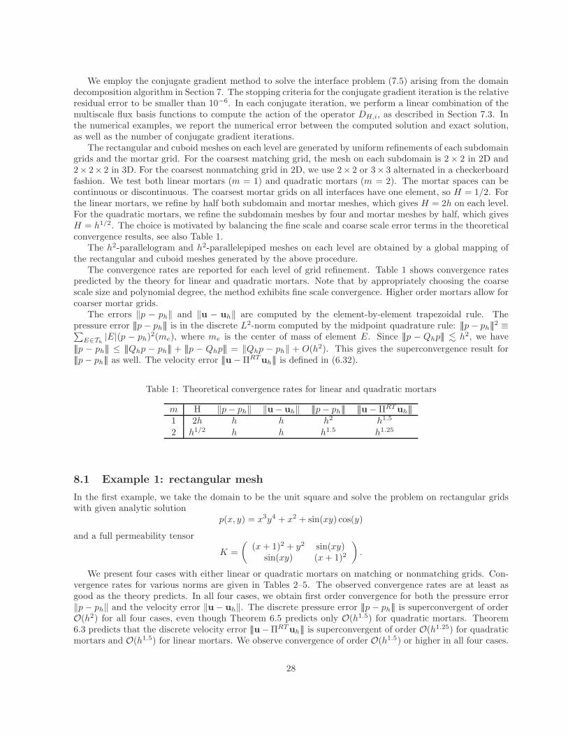
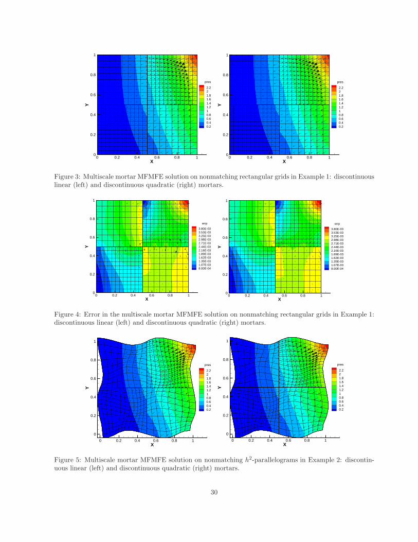
In terms of the computational cost, quadratic mortars are more efficient than linear mortars. Continuouslinear mortars need 50 CG iterations with h = 1/256, see Table 2, while continuous quadratic mortars requireonly 33 iterations on the same fine mesh level, as shown in Table 3. Similarly for the discontinuous case inTables 4 - 5, the CG iteration number with quadratic mortars is smaller than that with linear mortars. Thiscan be explained by the much coarser mortar grids used with quadratic mortars. The computed velocityand pressure with discontinuous linear and quadratic mortars on the same nonmatching grids are given inFigure 3. The numerical errors are given in Figure 4 accordingly. The errors are comparable, although asomewhat smaller velocity error along the interfaces is observed for quadratic mortars.

Table 2: Example 1: continuous linear mortars on matching grids

1/h ‖p− ph‖ ‖u− uh‖ |||p− ph||| |||u − ΠRTuh||| CGiter4 2.53E-01 — 1.06E+00 — 5.39E-02 — 1.27E-01 — 88 1.21E-01 1.06 5.23E-01 1.02 1.38E-02 1.97 3.10E-02 2.03 1116 5.96E-02 1.02 2.57E-01 1.03 3.46E-03 2.00 7.66E-03 2.02 1432 2.97E-02 1.00 1.27E-01 1.02 8.66E-04 2.00 1.92E-03 2.00 1864 1.48E-02 1.00 6.34E-02 1.00 2.16E-04 2.00 4.80E-04 2.00 26128 7.42E-03 1.00 3.16E-02 1.00 5.41E-05 2.00 1.20E-04 2.00 36256 3.71E-03 1.00 1.58E-02 1.00 1.36E-05 1.99 3.67E-05 1.71 50

Table 3: Example 1: continuous quadratic mortars on matching grids

1/h ‖p− ph‖ ‖u− uh‖ |||p− ph||| |||u − ΠRTuh||| CGiter4 2.53E-01 — 1.06E+00 — 5.39E-02 — 1.27E-01 — 816 5.96E-02 1.04 2.57E-01 1.02 3.46E-03 1.98 7.69E-03 2.02 1564 1.48E-02 1.00 6.34E-02 1.01 2.16E-04 2.00 5.71E-04 1.88 22256 3.71E-03 1.00 1.58E-02 1.00 1.36E-05 1.99 7.61E-05 1.45 33

Table 4: Example 1: discontinuous linear mortars on nonmatching grids

1/h ‖p− ph‖ ‖u− uh‖ |||p− ph||| |||u − ΠRTuh||| CGiter4 1.97E-01 — 7.59E-01 — 3.59E-02 — 1.61E-01 — 88 9.59E-02 1.04 3.69E-01 1.04 9.18E-03 1.97 5.02E-02 1.68 1316 4.76E-02 1.01 1.81E-01 1.03 2.31E-03 1.99 1.54E-02 1.70 1932 2.37E-02 1.01 8.99E-02 1.01 5.79E-04 2.00 4.82E-03 1.68 2864 1.19E-02 0.99 4.48E-02 1.00 1.45E-04 2.00 1.56E-03 1.63 41128 5.93E-03 1.00 2.24E-02 1.00 3.63E-05 2.00 5.18E-04 1.60 58256 2.97E-03 1.00 1.12E-02 1.00 9.10E-06 2.00 1.77E-04 1.55 85

8.2 Example 2: h2-parallelogram mesh

In the second example, we take the domain to be a C∞ map of the unit square. The map is defined as

x = x+ 0.03 cos(3πx) cos(3πy),

y = y − 0.04 cos(3πx) cos(3πy).

29

X

Y

0 0.2 0.4 0.6 0.8 10

0.2

0.4

0.6

0.8

1

pres

2.221.81.61.41.210.80.60.40.2

X

Y

0 0.2 0.4 0.6 0.8 10

0.2

0.4

0.6

0.8

1

pres

2.221.81.61.41.210.80.60.40.2

Figure 3: Multiscale mortar MFMFE solution on nonmatching rectangular grids in Example 1: discontinuouslinear (left) and discontinuous quadratic (right) mortars.

X

Y

0 0.2 0.4 0.6 0.8 10

0.2

0.4

0.6

0.8

1

errp

3.80E-033.53E-033.25E-032.98E-032.71E-032.44E-032.16E-031.89E-031.62E-031.35E-031.07E-038.00E-04

X

Y

0 0.2 0.4 0.6 0.8 10

0.2

0.4

0.6

0.8

1

errp

3.80E-033.53E-033.25E-032.98E-032.71E-032.44E-032.16E-031.89E-031.62E-031.35E-031.07E-038.00E-04

Figure 4: Error in the multiscale mortar MFMFE solution on nonmatching rectangular grids in Example 1:discontinuous linear (left) and discontinuous quadratic (right) mortars.

X

Y

0 0.2 0.4 0.6 0.8 1

0

0.2

0.4

0.6

0.8

1

pres

2.221.81.61.41.210.80.60.40.2

X

Y

0 0.2 0.4 0.6 0.8 1

0

0.2

0.4

0.6

0.8

1

pres

2.221.81.61.41.210.80.60.40.2

Figure 5: Multiscale mortar MFMFE solution on nonmatching h2-parallelograms in Example 2: discontin-uous linear (left) and discontinuous quadratic (right) mortars.

30

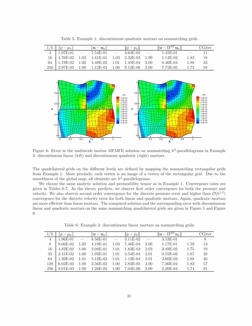
Table 5: Example 1: discontinuous quadratic mortars on nonmatching grids

1/h ‖p− ph‖ ‖u− uh‖ |||p− ph||| |||u − ΠRTuh||| CGiter4 1.97E-01 — 7.54E-01 — 3.64E-02 — 1.45E-01 — 1116 4.76E-02 1.02 1.81E-01 1.03 2.32E-03 1.99 1.14E-02 1.83 1864 1.19E-02 1.00 4.48E-02 1.01 1.45E-04 2.00 8.46E-04 1.88 33256 2.97E-03 1.00 1.12E-02 1.00 9.12E-06 2.00 7.75E-05 1.72 58

X

Y

0 0.2 0.4 0.6 0.8 1

0

0.2

0.4

0.6

0.8

1

errp

3.2E-032.9E-032.7E-032.4E-032.1E-031.8E-031.6E-031.3E-031.0E-037.5E-044.7E-042.0E-04

X

Y

0 0.2 0.4 0.6 0.8 1

0

0.2

0.4

0.6

0.8

1

errp

3.2E-032.9E-032.7E-032.4E-032.1E-031.8E-031.6E-031.3E-031.0E-037.5E-044.7E-042.0E-04

Figure 6: Error in the multiscale mortar MFMFE solution on nonmatching h2-parallelograms in Example2: discontinuous linear (left) and discontinuous quadratic (right) mortars.

The quadrilateral grids on the different levels are defined by mapping the nonmatching rectangular gridsfrom Example 1. More precisely, each vertex is an image of a vertex of the rectangular grid. Due to thesmoothness of the global map, all elements are h2-parallelograms.

We choose the same analytic solution and permeability tensor as in Example 1. Convergence rates aregiven in Tables 6-7. As the theory predicts, we observe first order convergence for both the pressure andvelocity. We also observe second order convergence for the discrete pressure error and higher than O(h1.5)convergence for the discrete velocity error for both linear and quadratic mortars. Again, quadratic mortarsare more efficient than linear mortars. The computed solution and the corresponding error with discontinuouslinear and quadratic mortars on the same nonmatching quadrilateral grids are given in Figure 5 and Figure6.

Table 6: Example 2: discontinuous linear mortars on nonmatching grids

1/h ‖p− ph‖ ‖u− uh‖ |||p− ph||| |||u − ΠRTuh||| CGiter4 1.96E-01 — 8.56E-01 — 3.11E-02 — 3.53E-01 — 88 9.66E-02 1.02 4.19E-01 1.03 7.46E-03 2.06 1.17E-01 1.59 1316 4.82E-02 1.00 2.08E-01 1.01 1.83E-03 2.03 3.49E-02 1.75 1932 2.41E-02 1.00 1.03E-01 1.01 4.54E-04 2.01 9.55E-03 1.87 2864 1.20E-02 1.01 5.13E-02 1.01 1.13E-04 2.01 2.60E-03 1.88 40128 6.02E-03 1.00 2.56E-02 1.00 2.82E-05 2.00 7.36E-04 1.83 57256 3.01E-03 1.00 1.28E-02 1.00 7.04E-06 2.00 2.20E-04 1.74 81

31

Table 7: Example 2: discontinuous quadratic mortars on nonmatching grids

1/h ‖p− ph‖ ‖u− uh‖ |||p− ph||| |||u − ΠRTuh||| CGiter4 1.96E-01 — 8.53E-01 — 3.16E-02 — 3.52E-01 — 1116 4.82E-02 1.01 2.07E-01 1.02 1.84E-03 2.05 3.32E-02 1.70 1764 1.20E-02 1.00 5.12E-02 1.01 1.13E-04 2.01 2.25E-03 1.94 32256 3.01E-03 1.00 1.28E-02 1.00 7.05E-06 2.00 1.52E-04 1.94 58

8.3 Example 3: cuboid mesh

In the third example, we consider cuboid grids on the unit cube with given analytic solution

p(x, y, z) = x+ y + z − 1.5,

and a full tensor coefficient

K =

x2 + y2 + 1 0 0

0 z2 + 1 sin(xy)0 sin(xy) x2y2 + 1

.

Convergence rates are reported in Tables 8 and 9. Again, these results confirm the theoretical results. Notethat the discrete velocity error |||u− ΠRT uh||| has second order of convergence for both linear and quadraticmortars on matching grids, even though the theory predicts O(h1.5) for linear mortars and O(h1.25) forquadratic mortars. The computed solution and its error for the case of discontinuous quadratic mortars areshown in Figure 7.

pres

1.210.80.60.40.20

-0.2-0.4-0.6-0.8-1-1.2

errp

9.0E-048.3E-047.5E-046.8E-046.1E-045.4E-044.6E-043.9E-043.2E-042.5E-041.7E-041.0E-04

Figure 7: Multiscale mortar MFMFE solution (left) and error (right) for Example 3: discontinuous quadraticmortars on matching grids

8.4 Example 4: regular h2-parallelepiped mesh

In this example, we take the domain to be a C∞ map of the unit cube. The map is defined as

x = x+ 0.03 cos(3πx) cos(3πy) cos(3πz),

y = y − 0.04 cos(3πx) cos(3πy) cos(3πz),

z = z + 0.05 cos(3πx) cos(3πy) cos(3πz).

32

pres

1.210.80.60.40.20

-0.2-0.4-0.6-0.8-1-1.2

errp

6.5E-036.0E-035.5E-035.0E-034.5E-034.0E-033.5E-033.0E-032.5E-032.0E-031.5E-031.0E-035.0E-04

Figure 8: Multiscale mortar MFMFE solution (left) and error (right) for Example 4: discontinuous quadraticmortars on matching grids

Table 8: Example 3: discontinuous linear mortars on matching grids

1/h ‖p− ph‖ ‖u− uh‖ |||p− ph||| |||u − ΠRTuh||| CGiter4 2.17E-01 — 1.55E-01 — 9.87E-03 — 3.73E-03 — 148 1.08E-01 1.01 7.76E-02 1.00 2.47E-03 2.00 1.03E-03 1.86 2016 5.41E-02 1.00 3.88E-02 1.00 6.17E-04 2.00 2.60E-04 1.99 2832 2.71E-02 1.00 1.94E-02 1.00 1.54E-04 2.00 6.50E-05 2.00 3964 1.35E-02 1.01 9.68E-03 1.00 3.85E-05 2.00 1.66E-05 1.97 56

Table 9: Example 3: discontinuous quadratic mortars on matching grids

1/h ‖p− ph‖ ‖u− uh‖ |||p− ph||| |||u − ΠRTuh||| CGiter4 2.17E-01 — 1.55E-01 — 9.87E-03 — 3.73E-03 — 1416 5.41E-02 1.00 3.88E-02 1.00 6.17E-04 2.00 2.61E-04 1.92 2764 1.35E-02 1.00 9.68E-03 1.00 3.85E-05 2.00 1.67E-05 1.98 53

Table 10: Example 4: discontinuous linear mortars on matching grids

1/h ‖p− ph‖ ‖u− uh‖ |||p− ph||| |||u − ΠRTuh||| CGiter4 2.18E-01 — 2.82E-01 — 1.39E-02 — 7.48E-02 — 148 1.10E-01 0.99 1.66E-01 0.76 5.07E-03 1.46 5.15E-02 0.54 2016 5.49E-02 1.00 8.96E-02 0.89 1.86E-03 1.45 2.09E-02 1.30 2832 2.75E-02 1.00 4.51E-02 0.99 5.24E-04 1.83 5.93E-03 1.82 4064 1.37E-02 1.01 2.23E-02 1.02 1.35E-04 1.96 1.52E-03 1.96 57

The computational grids are defined by mapping the cuboid grids considered in Example 3. Each vertexof a hexahedral element is obtained by mapping a vertex in the cuboid grid. The element trilinear map-ping determines the shape of each hexahedron. The smoothness of the global mapping implies that eachhexahedron is a regular h2-parallelepiped.

33

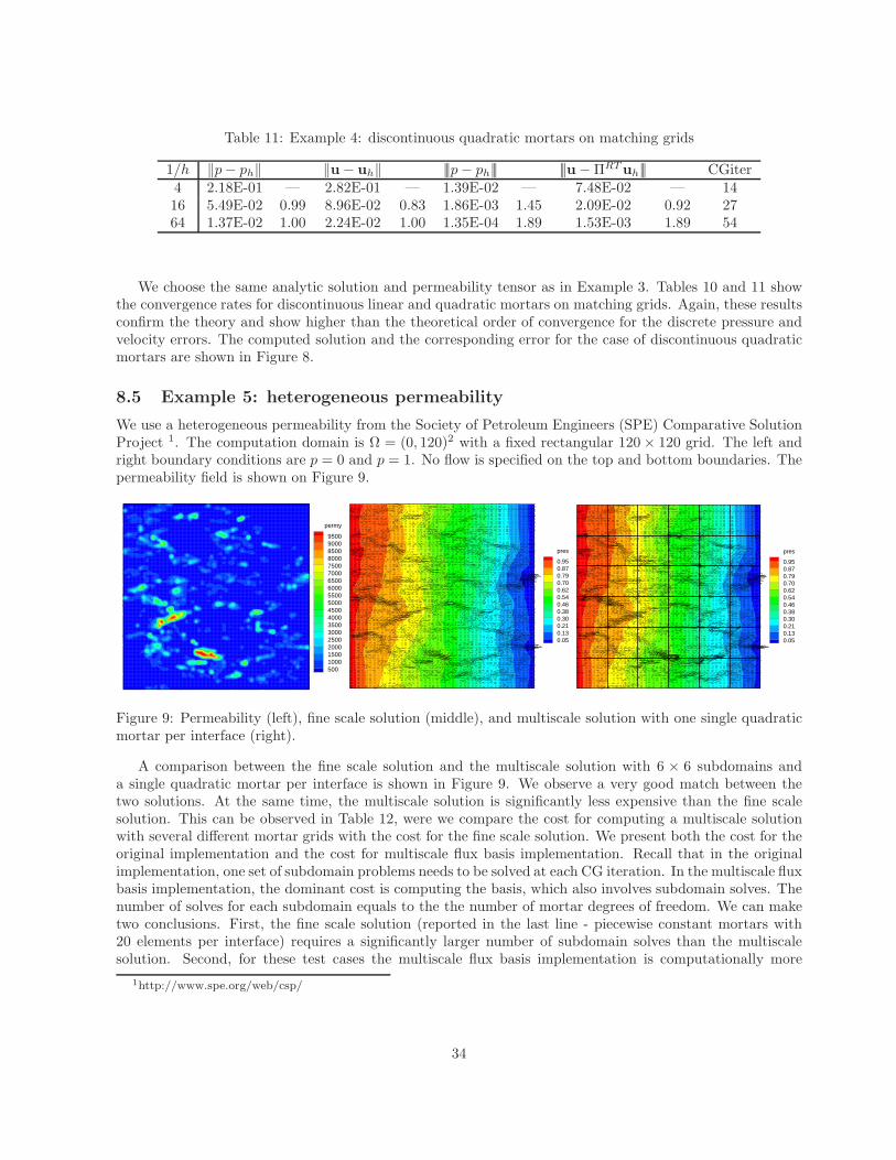
Table 11: Example 4: discontinuous quadratic mortars on matching grids

1/h ‖p− ph‖ ‖u− uh‖ |||p− ph||| |||u − ΠRTuh||| CGiter4 2.18E-01 — 2.82E-01 — 1.39E-02 — 7.48E-02 — 1416 5.49E-02 0.99 8.96E-02 0.83 1.86E-03 1.45 2.09E-02 0.92 2764 1.37E-02 1.00 2.24E-02 1.00 1.35E-04 1.89 1.53E-03 1.89 54

We choose the same analytic solution and permeability tensor as in Example 3. Tables 10 and 11 showthe convergence rates for discontinuous linear and quadratic mortars on matching grids. Again, these resultsconfirm the theory and show higher than the theoretical order of convergence for the discrete pressure andvelocity errors. The computed solution and the corresponding error for the case of discontinuous quadraticmortars are shown in Figure 8.

8.5 Example 5: heterogeneous permeability

We use a heterogeneous permeability from the Society of Petroleum Engineers (SPE) Comparative SolutionProject 1. The computation domain is Ω = (0, 120)2 with a fixed rectangular 120 × 120 grid. The left andright boundary conditions are p = 0 and p = 1. No flow is specified on the top and bottom boundaries. Thepermeability field is shown on Figure 9.

permy

950090008500800075007000650060005500500045004000350030002500200015001000500

pres

0.950.870.790.700.620.540.460.380.300.210.130.05

pres

0.950.870.790.700.620.540.460.380.300.210.130.05

Figure 9: Permeability (left), fine scale solution (middle), and multiscale solution with one single quadraticmortar per interface (right).

A comparison between the fine scale solution and the multiscale solution with 6 × 6 subdomains anda single quadratic mortar per interface is shown in Figure 9. We observe a very good match between thetwo solutions. At the same time, the multiscale solution is significantly less expensive than the fine scalesolution. This can be observed in Table 12, were we compare the cost for computing a multiscale solutionwith several different mortar grids with the cost for the fine scale solution. We present both the cost for theoriginal implementation and the cost for multiscale flux basis implementation. Recall that in the originalimplementation, one set of subdomain problems needs to be solved at each CG iteration. In the multiscale fluxbasis implementation, the dominant cost is computing the basis, which also involves subdomain solves. Thenumber of solves for each subdomain equals to the the number of mortar degrees of freedom. We can maketwo conclusions. First, the fine scale solution (reported in the last line - piecewise constant mortars with20 elements per interface) requires a significantly larger number of subdomain solves than the multiscalesolution. Second, for these test cases the multiscale flux basis implementation is computationally more

1http://www.spe.org/web/csp/

34

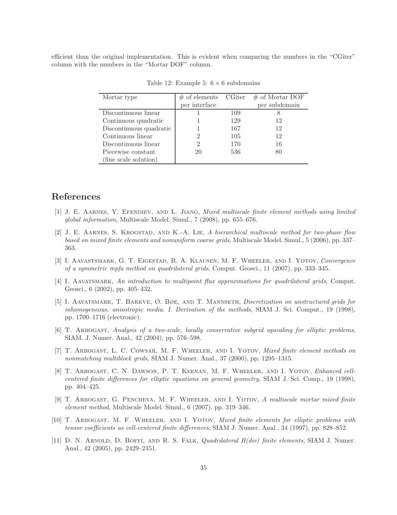
efficient than the original implementation. This is evident when comparing the numbers in the “CGiter”column with the numbers in the “Mortar DOF” column.

Table 12: Example 5: 6 × 6 subdomains

Mortar type # of elements CGiter # of Mortar DOFper interface per subdomain

Discontinuous linear 1 109 8Continuous quadratic 1 129 12Discontinuous quadratic 1 167 12Continuous linear 2 105 12Discontinuous linear 2 170 16Piecewise constant 20 536 80(fine scale solution)

References

[1] J. E. Aarnes, Y. Efendiev, and L. Jiang, Mixed multiscale finite element methods using limitedglobal information, Multiscale Model. Simul., 7 (2008), pp. 655–676.

[2] J. E. Aarnes, S. Krogstad, and K.-A. Lie, A hierarchical multiscale method for two-phase flowbased on mixed finite elements and nonuniform coarse grids, Multiscale Model. Simul., 5 (2006), pp. 337–363.

[3] I. Aavastsmark, G. T. Eigestad, R. A. Klausen, M. F. Wheeler, and I. Yotov, Convergenceof a symmetric mpfa method on quadrilateral grids, Comput. Geosci., 11 (2007), pp. 333–345.

[4] I. Aavatsmark, An introduction to multipoint flux approximations for quadrilateral grids, Comput.Geosci., 6 (2002), pp. 405–432.

[5] I. Aavatsmark, T. Barkve, Ø. Bøe, and T. Mannseth, Discretization on unstructured grids forinhomogeneous, anisotropic media. I. Derivation of the methods, SIAM J. Sci. Comput., 19 (1998),pp. 1700–1716 (electronic).

[6] T. Arbogast, Analysis of a two-scale, locally conservative subgrid upscaling for elliptic problems,SIAM. J. Numer. Anal., 42 (2004), pp. 576–598.

[7] T. Arbogast, L. C. Cowsar, M. F. Wheeler, and I. Yotov, Mixed finite element methods onnonmatching multiblock grids, SIAM J. Numer. Anal., 37 (2000), pp. 1295–1315.

[8] T. Arbogast, C. N. Dawson, P. T. Keenan, M. F. Wheeler, and I. Yotov, Enhanced cell-centered finite differences for elliptic equations on general geometry, SIAM J. Sci. Comp., 19 (1998),pp. 404–425.

[9] T. Arbogast, G. Pencheva, M. F. Wheeler, and I. Yotov, A multiscale mortar mixed finiteelement method, Multiscale Model. Simul., 6 (2007), pp. 319–346.

[10] T. Arbogast, M. F. Wheeler, and I. Yotov, Mixed finite elements for elliptic problems withtensor coefficients as cell-centered finite differences, SIAM J. Numer. Anal., 34 (1997), pp. 828–852.

[11] D. N. Arnold, D. Boffi, and R. S. Falk, Quadrilateral H(div) finite elements, SIAM J. Numer.Anal., 42 (2005), pp. 2429–2451.

35

[12] D. N. Arnold and F. Brezzi, Mixed and nonconforming finite element methods: implementation,postprocessing and error estimates, RAIRO Model. Math. Anal. Numer., 19 (1985), pp. 7–32.

[13] J. Baranger, J. F. Maitre, and F. Oudin, Connection between finite volume and mixed finiteelement methods, RAIRO Model. Math. Anal. Numer., 30 (1996), pp. 445–465.

[14] C. Bernardi, Y. Maday, and A. T. Patera, A new nonconforming approach to domain decomposi-tion: The mortar element method, in Nonlinear Partial Differential Equations and Their Applications,H. Brezis and J. L. Lions eds., Longman Scientific and Technical, Harlow, UK, 1994.

[15] M. Berndt, K. Lipnikov, M. Shashkov, M. F. Wheeler, and I. Yotov, Superconvergence ofthe velocity in mimetic finite difference methods on quadrilaterals, SIAM. J. Numer. Anal., 43 (2005),pp. 1728–1749.

[16] S. C. Brenner and L. R. Scott, The Mathematical Theory of Finite Element Methods, Texts inApplied Mathematics, Springer-Verlag, 2007.

[17] F. Brezzi, J. Douglas, R. Duran, and M. Fortin, Mixed finite elements for second order ellipticproblems in three variables, Numer. Math., 51 (1987), pp. 237–250.

[18] F. Brezzi, J. Douglas, and L. D. Marini, Two families of mixed finite elements for second orderelliptic problems, Numer. Math., 47 (1985), pp. 217–235.

[19] F. Brezzi and M. Fortin, Mixed and hybrid finite element methods, Spring-Verlag, New York, 1991.

[20] F. Brezzi, M. Fortin, and L. D. Marini, Error analysis of piecewise constant pressure approxima-tions of Darcy’s law, Comp. Meth. Appl. Mech. Engng., 195 (2006), pp. 1547–1559.

[21] Z. Cai, J. E. Jones, S. F. McCormick, and T. F. Russell, Control-volume mixed finite elementmethods, Comput. Geosci., 1 (1997), pp. 289–315 (1998).

[22] Z. Chen and T. Y. Hou, A mixed multiscale finite element method for elliptic problems with oscillatingcoefficients, Math. Comp., 72 (2003), pp. 541–576.

[23] P. G. Ciarlet, The Finite Element Method for Elliptic Problems, Stud. Math. Appl. 4, North-Holland,Amsterdam, 1978; reprinted, SIAM, Philadelphia, 2002.

[24] R. Duran, Superconvergence for rectangular mixed finite elements, Numer. Math., 58 (1990), pp. 287–298.

[25] M. G. Edwards, Unstructured, control-volume distributed, full-tensor finite-volume schemes with flowbased grids, Comput. Geosci., 6 (2002), pp. 433–452.

[26] M. G. Edwards and C. F. Rogers, Finite volume discretization with imposed flux continuity for thegeneral tensor pressure equation, Comput. Geosci., 2 (1998), pp. 259–290 (1999).

[27] R. E. Ewing, M. M. Liu, and J. Wang, Superconvergence of mixed finite element approximationsover quadrilaterals, SIAM. J. Numer. Anal., 36 (1999), pp. 772–787.

[28] R. Eymad, T. Gallouet, and R. Herbin, Finite volume methods, in Handbook of Numerical Anal-ysis, North-Holland, Amsterdam, (2000), pp. 713–1020.

[29] G. P. Galdi, An introduction to the mathematical theory of the Navier-Stokes equations. Vol. I,Springer-Verlag, New York, 1994. Linearized steady problems.

[30] B. Ganis and I. Yotov, Implementation of a mortar mixed finite element using a multiscale fluxbasis, Comput. Methods Appl. Mech. Engrg., (2009), pp. 3989–3998.

36

[31] V. Girault and P. A. Raviart, Finite Element Methods for Navier-Stokes Equations, Theory andAlgorithms., Spring-Verlag, 1986.

[32] R. Glowinski and M. F. Wheeler, Domain decomposition and mixed finite element methods for el-liptic problems, in First International Symposium on Domain Decomposition Methods for Partial Differ-ential Equations, R. Glowinski, G. H. Golub, G. A. Meurant, and J. Periaux, eds., SIAM, Philadelphia,1988, pp. 144–172.

[33] P. Grisvard, Elliptic Problems in Nonsmooth Domains, Pitman, Boston, MA, 1995.

[34] T. Y. Hou and X. H. Wu, A multiscale finite element method for elliptic problems in compositematerials and porous media, J. Comput. Phys., 134 (1997), pp. 169–189.

[35] T. J. R. Hughes, G. R. Feijoo, L. Mazzei, and J.-B. Quincy, The variational multiscale method–aparadim for computational mechanics, Comp. Meth. Appl. Mech. Engng., 166 (1998), pp. 3–24.

[36] J. Hyman, M. Shashkov, and S. Steinberg, The numerical solution of diffusion problem in stronglyheterogeneous non-isotropic materials, J. Comput. Phys., 132 (1997), pp. 130–148.

[37] R. Ingram, M. F. Wheeler, and I. Yotov, A multipoint flux mixed finite element method onhexahedra, To appear in SIAM J. Numer. Anal., (2010).

[38] P. Jenny, S. H. Lee, and H. A. Tchelepi, Multi-scale finite-volume method for elliptic problems insubsurface flow simulation, J. Comput. Phys., 187 (2003), pp. 47–67.

[39] R. A. Klausen and R. Winther, Convergence of multipoint flux approximations on quadrilateralgrids, Numer. Methods Partial Differential Equations, 22 (2006), pp. 1438–1454.

[40] R. A. Klausen and R. Winther, Robust convergence of multi point flux approximation on roughgrids, Numer. Math., 104 (2006), pp. 317–337.

[41] J. L. Lions and E. Magenes, Non-homogeneous Boundary Value Problems and Applications,Springer-Verlag Berlin Heidelberg New York, 1972.

[42] K. Lipnikov, M. Shashkov, and I. Yotov, Local flux mimetic finite difference methods, Numer.Math., 112 (2009), pp. 115–152.

[43] T. P. Mathew, Domain Decomposition and Iterative Methods for Mixed Finite Element Discretiza-tions of Elliptic Problems, Tech. Report 463, Courant Institute of Mathematical Sciences, New YorkUniversity, New York, 1989.

[44] J. C. Nedelec, Mixed finite elements in R3, Numer. Math., 35 (1980), pp. 315–341.

[45] P. A. Raviart and J. Thomas, A mixed finite element method for 2-nd order elliptic problems, inMathematical aspects of the Finite Elements Method, I. Galligani and E. Magenes, eds., Lectures Notesin Math. 606, Springer, Berlin, 1977, pp. 292–315.

[46] J. E. Roberts and J.-M. Thomas, Mixed and hybrid methods, in Handbook of Numerical Analysis,Vol. II, P. G. Ciarlet and J. Lions, eds., Elsevier Science Publishers B.V., 1991, pp. 523–639.

[47] T. F. Russell and M. F. Wheeler, Finite element and finite difference methods for continuous flowsin porous media, in The Mathematics of Reservoir Simulation, R. E. Ewing, ed., SIAM, Philadelphia,1983, pp. 35–106.

[48] R. Scott and S. Zhang, Finite element interpolation of nonsmooth functions satisfying boundaryconditions, Math. Comp., 54 (1990), pp. 483–493.

[49] J. M. Thomas, These de doctorat d’etat, ’a I’Universite Pierre et Marie Curie, (1977).

37

[50] J. Wang and T. P. Mathew, Mixed finite element method over quadrilaterals, in Conference onAdvances in Numerical Methods and Applications, I. T. Dimov, B. Sendov, and P. Vassilevski, eds.,World Scientific, River Edge, NJ, (1994), pp. 351–375.

[51] A. Weiser and M. F. Wheeler, On convergence of block-centered finite differences for elliptic prob-lems, SIAM J. Numer. Anal., 25 (1988), pp. 351–375.

[52] M. F. Wheeler, G. Xue, and I. Yotov, A multipoint flux mixed finite element method on distortedquadrilaterals and hexahedra, Preprint, (2010).

[53] M. F. Wheeler and I. Yotov, A multipoint flux mixed finite element method, SIAM. J. Numer.Anal., 44 (2006), pp. 2082–2106.

38