JOURNAL OF COMPUTATIONAL PHYSICS 134, 169–189 (1997)ARTICLE NO. CP975682

A Multiscale Finite Element Method for Elliptic Problems inComposite Materials and Porous Media

Thomas Y. Hou and Xiao-Hui Wu

Applied Mathematics, Caltech, Pasadena, California 91125

Received August 5, 1996

A direct numerical solution of the multiple scale prob-lems is difficult even with modern supercomputers. TheIn this paper, we study a multiscale finite element method for

solving a class of elliptic problems arising from composite materials major difficulty of direct solutions is the scale of computa-and flows in porous media, which contain many spatial scales. The tion. For groundwater simulations, it is common to havemethod is designed to efficiently capture the large scale behavior millions of grid blocks involved, with each block having aof the solution without resolving all the small scale features. This

dimension of tens of meters, whereas the permeabilityis accomplished by constructing the multiscale finite element basefunctions that are adaptive to the local property of the differential measured from cores is at a scale of several centimetersoperator. Our method is applicable to general multiple-scale prob- [23]. This gives more than 105 degrees of freedom perlems without restrictive assumptions. The construction of the base spatial dimension in the computation. Therefore, a tremen-functions is fully decoupled from element to element; thus, the

dous amount of computer memory and CPU time are re-method is perfectly parallel and is naturally adapted to massivelyquired, and they can easily exceed the limit of today’sparallel computers. For the same reason, the method has the ability

to handle extremely large degrees of freedom due to highly hetero- computing resources. The situation can be relieved to somegeneous media, which are intractable by conventional finite element degree by parallel computing; however, the size of discrete(difference) methods. In contrast to some empirical numerical problem is not reduced. The load is merely shared by moreupscaling methods, the multiscale method is systematic and self-

processors with more memory. Some recent direct solu-consistent, which makes it easier to analyze. We give a brief analysisof the method, with emphasis on the ‘‘resonant sampling’’ effect. tions of flow and transport in porous media are reportedThen, we propose an oversampling technique to remove the reso- in [1, 25, 9, 22]. Whenever one can afford to resolve all thenance effect. We demonstrate the accuracy and efficiency of our small scale features of a physical problem, direct solutionsmethod through extensive numerical experiments, which include

provide quantitative information of the physical processesproblems with random coefficients and problems with continuousat all scales. On the other hand, from an engineering per-scales. Parallel implementation and performance of the method are

also addressed. Q 1997 Academic Press spective, it is often sufficient to predict the macroscopicproperties of the multiple-scale systems, such as the effec-tive conductivity, elastic moduli, permeability, and eddy

1. INTRODUCTION diffusivity. Therefore, it is desirable to develop a methodthat captures the small scale effect on the large scales, butMany problems of fundamental and practical impor-which does not require resolving all the small scale fea-tance have multiple-scale solutions. Composite materials,tures.porous media, and turbulent transport in high Reynolds

Here, we study a multiscale finite element methodnumber flows are examples of this type. A complete analy-(MFEM) for solving partial differential equations withsis of these problems is extremely difficult. For example,multiscale solutions. The central goal of this approach isthe difficulty in analyzing groundwater transport is mainlyto obtain the large scale solutions accurately and efficientlycaused by the heterogeneity of subsurface formations span-without resolving the small scale details. The main idea isning over many scales [7]. The heterogeneity is often repre-to construct finite element base functions which capturesented by the multiscale fluctuations in the permeabilitythe small scale information within each element. The smallof the media. For composite materials, the dispersed phasesscale information is then brought to the large scales(particles or fibers), which may be randomly distributedthrough the coupling of the global stiffness matrix. Thus,in the matrix, give rise to fluctuations in the thermal orthe effect of small scales on the large scales is correctlyelectrical conductivity; moreover, the conductivity is usu-captured. In our method, the base functions are con-ally discontinuous across the phase boundaries. In turbu-structed from the leading order homogeneous elliptic equa-lent transport problems, the convective velocity field fluc-tion in each element. As a consequence, the base functionstuates randomly and contains many scales depending on

the Reynolds number of the flow. are adapted to the local properties of the differential opera-

1690021-9991/97 $25.00

Copyright 1997 by Academic PressAll rights of reproduction in any form reserved.

170 HOU AND WU

tor. In the case of two-scale periodic structures, Hou, Wu, although the homogenization theory helps reveal the causeof the problem. This makes it possible to generalize ourand Cai have proved that the multiscale method indeed

converges to the correct solution independent of the small method to problems with continuous scales. We will dem-onstrate through extensive numerical experiments that thisscale in the homogenization limit [21].

In this paper, we continue the study of the multiscale simple technique is very effective for a wide range of appli-cations, including problems with random coefficients andmethod, with emphasis on problems with continuous scales

from composite materials and flows in porous media. Ex- problems with continuous scales.In practical computations, a large amount of overheadtensive numerical tests are performed on these problems.

The error analysis of the method is reviewed briefly time comes from constructing the base functions. Thesemultiscale base functions are constructed numerically,for problems with scale separation. The accuracy of our

method for problems with continuous scales is then studied except for certain special cases. Since the base functionsare independent of each other, they can be constructednumerically. Moreover, we compare our method with tra-

ditional finite element (difference) methods as well as ex- independently and this can be done perfectly in parallel.This greatly reduces the overhead time in constructingisting numerical upscaling methods in terms of operation

counts and memory requirement. We give two simple par- these bases. On a sequential machine, the operation countof our method is about twice that of a conventional finiteallel implementations of our method and study their paral-

lel efficiency computationally. element method (FEM) for a 2D problem. The differenceis reduced significantly for a massively parallel computer.A common difficulty in numerical upscaling methods is

that large errors result from the ‘‘resonance’’ between the For example, running on 256 processors, our method onlyspends 9% more CPU time than a FEM using 1024 3 1024grid scale and the scales of the continuous problem. This

is revealed by our earlier analysis [21]. For the two-scale linear elements (see Section 4.6).Another advantage of our method is its ability to reduceproblem, the error due to the resonance manifests as a

ratio between the wavelength of the small scale oscillation the size of a large scale computation. This offers a bigsaving in computer memory. For example, let N be theand the grid size; the error becomes large when the two

scales are close. A deeper analysis shows that the boundary number of elements in each spatial direction, and let Mbe the number of subcell elements in each direction forlayer in the first-order corrector seems to be the main

source of the resonance effect. By a judicious choice of solving the base functions. Then there are total (M N)n

(n is the dimension) elements at the fine grid level. For aboundary conditions for the base function, we can elimi-nate the boundary layer in the first-order corrector. This traditional FEM, the computer memory needed for solving

the problem on the fine grid is O(M n N n ). In contrast,would give a nice conservative difference structure in thediscretization, which in turn leads to cancellation of reso- MFEM requires only O(M n 1 N n ) amount of memory.

If M 5 32 in a 2D problem, then traditional FEM needsnance errors and gives an improved rate of convergenceindependent of the small scales in the solution. about 1000 times more memory than MFEM.

Since we need to use an additional grid to compute theMotivated by our earlier analysis [21] mentioned above,here we propose an over-sampling method to overcome base function numerically, it makes sense to compare our

multiscale FEM with a traditional FEM at the subcell grid,the difficulty due to scale resonance. The idea is quitesimple and easy to implement. Since the boundary layer hs 5 h/M. Note that the multiscale FEM only captures the

solution at the coarse grid h, while a traditional FEM triesin the first-order corrector is thin, O(«), we can sample ina domain with a size larger than h 1 « and use only the to resolve the solution at the fine grid hs 5 h/M. Our

extensive numerical experiments demonstrate that the ac-interior sampled information to construct the bases (seeSection 3.3). Here, h is the mesh size and « is the small curacy of our multiscale FEM on the coarse grid h is com-

parable to that of FEM on the fine grid. In some cases,scale in the solution. By doing this, the boundary layer inthe larger domain has no influence on the base functions. MFEM is even more accurate than FEM (see Sections 4.3

and 4.4).Now the corresponding first-order correctors are free ofboundary layers. As a result, we obtain an improved rate At this point, we would like to emphasize that the pur-

pose of our method is to solve practical problems which areof convergence which is independent of the small scale.From practical considerations, this improvement is cru- too large to handle by direct methods on given computing

resources. Our method gives a systematic and self-consis-cial. For problems with many scales or continuous scales,it is inevitable to have the mesh size h coincide with one of tent approach to capture the large scale solution correctly

without resolving the small scale details and withoutthe physical scales. Without this improvement, we cannotguarantee that our method converges completely indepen- resorting to closure arguments. We show that at a reason-

able cost, the multiscale FEM has the ability to solve verydent of the small scale features in the solution. It is alsoimportant that our oversampling technique does not rely large scale practical problems with accuracy comparable

to the corresponding direct simulations at the fine grid.on the homogenization theory (like solving a cell problem),

MULTISCALE FINITE ELEMENT METHOD 171

This gives hope to solving some large scale computational scale and the physical scale never occur in the correspond-ing 1D problems.problems that are otherwise intractable using direct

This paper is organized as follows. The formulation ofmethods.the 2D multiple-scale elliptic problem and the multiscaleIt should be mentioned that many numerical methodsfinite element method are given in the next section. Inhave been developed with goals similar to ours. TheseSection 3, we present the rationale behind the method,include methods based on the homogenization theoryincluding a brief review of the homogenization theory and(cf. [14, 10]), and some upscaling methods based on simpleconvergence analysis. The resonance effect is analyzed andphysical and/or mathematical motivations (cf. [12, 23]).the oversampling technique is proposed. More detailedThe methods based on the homogenization theory havenumerical analysis of the method is given in a separatebeen successfully applied to determining the effective con-paper [21]. The numerical implementation of the method,ductivity and permeability of certain composite materialsits convergence, and parallel performance are studied inand porous media [14, 10]. However, their range of applica-Section 4. Section 5 contains the application of thetions is usually limited by restrictive assumptions on themultiscale method to more practical problems in compositemedia, such as scale separation and periodicity [8]. Asmaterials and porous media flows, including steady conduc-discussed in Section 4.2, they are also expensive to use fortion through fiber composites and flows through randomsolving problems with many separate scales since the costporous media with normal and fractal porosity distribu-of computation grows exponentially with the number oftions. Using these examples, we show the adaptability ofscales. But for the multiscale method, the number of scalesthe method, its ability to solve large practical problems,is irrelevant to the computational cost. The upscaling meth-and its accuracy for general problems. Section 6 is reservedods are more general and have been applied to problemsfor some concluding remarks and discussion of futurewith random coefficients with partial success (cf. [12, 23]).work.But the design principle is strongly motivated by the

homogenization theory for periodic structures. Their appli-2. FORMULATIONScations to nonperiodic structures are not always guaran-

teed to work.In this section, we introduce the elliptic problem andThere has also been success in achieving numerical ho-

the multiscale method. First, we state some notations andmogenization for some semilinear hyperbolic systems, theconventions to be used in the paper. In the following,incompressible Euler equations, and 1D elliptic problemsthe Einstein summation convention is used; summation is

using the sampling technique; see, e.g., [17, 15, 2]. Thistaken over repeated indices. Some notations of functional

technique has its own limitations. Its application to generalspaces will be used occasionally for the convenience of

2D elliptic problems is still not satisfactory. For fully ran- expressing the formulation and some relevant analyticaldom media, statistical theory and renormalization group estimates about the multiscale method. L2(V) denotes thetheory have been used to obtain the effective properties. space of square integrable functions defined in domain V.However, these methods usually become difficult to apply We use L2(V) based Sobolev spaces Hk(V) equipped withwhen the integral scale of correlation is large (Ref. [23] norms and seminorms given byand references therein). Moreover, certain simplifying as-sumptions in the underlying physics are usually made in

iui2k,V 5 E

VO

uau#kuDauu2, uuu2k,V 5 E

VO

uau5kuDauu2,order to obtain a closure of the effective equations. In

comparison, such a closure problem is not present in themultiscale method.

where Dau denotes the ath order mixed derivatives of u.We remark that the idea of using base functions gov-H1

0(V) consists of those functions in H1(V) that vanisherned by the differential equations has been applied toon ­V.

convection–diffusion equation with boundary layers (see,e.g., [6] and references therein). With a motivation differ- 2.1. Governing Equations and the Multiscale Finiteent from ours, Babuska et al. applied a similar idea to 1D Element Methodproblems [5] and to a special class of 2D problems with

We consider solving the second-order elliptic equationthe coefficient varying locally in one direction [4]. How-ever, most of these methods are based on the special prop-

2= ? a(x)=u 5 f in V, (2.1)erty of the harmonic average in one-dimensional ellipticproblems. As indicated by our convergence analysis, thereis a fundamental difference between one-dimensional where a(x) 5 (aij (x)) is the conductivity tensor and isproblems and genuinely multidimensional problems. Spe- assumed to be symmetric and positive definite with upper

and lower bounds. In the context of porous flows, Eq.cial complications such as the resonance between the mesh

172 HOU AND WU

(2.1) is the pressure equation for single phase steady flow element K [ K h, we define a set of nodal basis hfiK , i 5

1, ..., d j with d being the number of nodes of the element.through a porous medium. Correspondingly, a is the ratioof the permeability tensor k and the fluid viscosity e, and The subscript K will be neglected when bases in one

element are considered. In our multiscale method, fiu represents the pressure. The steady velocity field is re-lated to the pressure through Darcy’s law: satisfies

q 5 21e

k=u 5 2a=u (2.2)= ? a(x)=fi 5 0 in K [ K h. (2.4)

In this paper, we assume e 5 1 for convenience. Equation(2.1) is also the equation of steady state heat (electrical) Let xj [ K ( j 5 1, ..., d) be the nodal points of K. Asconduction through a composite material, with a and u usual, we require fi(xj) 5 dij . One needs to specify theinterpreted as the thermal (electric) conductivity and tem- boundary condition of fi to make (2.4) a well-posed prob-perature (electric potential). In practice, a may be random lem (see below). For now, we assume that the base func-or highly oscillatory; thus the solution of (2.1) displays a tions are continuous across the boundaries of the elements,multiple scale structure. Since for the transient problem so thatthe main difficulty is the same as that for the steady stateproblem, i.e., the multiple scales in the solution, we onlyconsider solving the steady problem here. The multiscale V h 5 spanhfi

K : i 5 1, ..., d; K [ K hj , H10(V).

method, however, can be easily extended to solve the tran-sient problems.

In the following, we study the approximate solution ofTo simplify the presentation of the finite element formu-(2.3) in V h, i.e., uh [ V h such thatlation, we assume u 5 0 on ­V and that the solution domain

is a unit square V 5 (0, 1) 3 (0, 1). The variational problemof (2.1) is to seek u [ H1

0(V) such thata(uh, v) 5 f (v) ;v [ V h. (2.5)

a(u, v) 5 f (v) ;v [ H10(V), (2.3)

where Note that this formulation of the multiscale method is notrestricted to rectangular elements. It can also be applied

a(u, v) 5 EV

aij­v­xi

­u­xj

dx, f (v) 5 EV

fv dx. to triangular elements (see Fig. 2.1) which are more flexiblein modeling complicated geometries.

A finite element method is obtained by restricting theweak formulation (2.3) to a finite-dimensional subspace of 2.2. The Boundary Condition of Base FunctionsH1

0(V). For 0 , h # 1, let K h be a partition of V by aThe important role of the boundary condition of thecollection of rectangles K with diameter #h, which is de-

base functions is obvious since the base functions satisfyfined by an axi-parallel rectangular mesh (Fig. 2.1). In eachthe homogeneous equation (2.4). We will see later that agood choice of the boundary condition can significantlyimprove the accuracy of the multiscale method. In fact,the boundary condition determines how well the localproperty of the operator is sampled into the base functions(see Section 3). Here, we describe two methods of imposingthe boundary condition, which are easy to implement andto analyze.

Denote ei 5 fiu­K . One choice is to let ei vary linearlyalong ­K, just as in the standard bilinear (linear) basefunctions. Another more appealing approach is to chooseei to be the solution of some reduced elliptic problems oneach side of ­K. The reduced problems are obtained from(2.4) by deleting terms with partial derivatives in the direc-tion normal to ­K and having the coordinate normal to­K as a parameter. It is clear that the reduced problemsare of the same form as (2.4). When a is separable in space,

FIG. 2.1. Rectangular mesh with triangulation. i.e., a(x) 5 a1(x)a2(y), fi can be computed analytically

MULTISCALE FINITE ELEMENT METHOD 173

Thus, the constant functions belong to V h. Later, we seethat this property is useful in discrete error cancellations.The generalization of the reduced problems, e.g., (2.6), tomore general elements, such as the triangular elements, isstraightforward.

2.3. Some General Remarks

The multiscale method formulated above is designed tocapture the large scale solutions. Unlike existing numericalupscaling methods, our method is consistent with the tradi-tional finite element method in a well-resolved computa-tion. It is proved in [21] that the multiscale method givesthe same rate of convergence as the linear finite element

FIGURE 2.2 method when the small scales are well resolved, h ! «.In particular, when the coefficient is a diagonal constantmatrix, the base functions constructed from (2.4) are noth-ing but the usual bilinear (linear) base functions. When h

from the tensor product of ei along Gi21 and Gi (note that does not resolve the small scales, the multiscale methodG0 ; G4 ; see Fig. 2.2). Furthermore, it can be shown that and the traditional finite element method behave very dif-this boundary condition is optimum for the space-separa- ferently. It is easy to show that the traditional finite elementble problems. methods do not converge to the correct solution. By con-

To be more specific, consider an element K [ K h with trast, the multiscale method captures the correct largenodal points xi 5 (xi , yi) (i 5 1, ..., d), which are labeled scale solutions.counterclockwise, starting from the lower left corner (Fig. As indicated by our analysis and numerical experiments2.2). On G1 and G3 , we have ei 5 ei(x) and in [21], the boundary condition of the base functions can

have a big influence on the accuracy of the multiscalemethod. From our computational experience, we found­

­xae(x)

­ei(x)­x

5 0, (2.6)that the oscillatory boundary condition for the base func-tions in general leads to better accuracy than the linearboundary condition. However, the multiscale method inwhere ae(x) 5 a11uG1

and a11uG3, respectively. Note that ae

general may fail to converge when the mesh scale is closeis bounded from above and below by positive constants.to the physical small scale due to a resonance betweenSimilarly, on G2 and G4 , we have ei 5 ei(y) andthese two scales. For the two-scale problem, the error dueto the resonance manifests as a ratio between the wave-­

­yae(y)

­ei(y)­y

5 0 length of the small scale oscillation and the grid size. Moti-vated by our earlier analysis [21], we propose in Section4.4 an oversampling method to overcome the difficulty due

with ae(y) 5 a22uG2and a22uG4

, respectively. The bound- to scale resonance.ary condition of these 1D elliptic equations is given byei(xj) 5 dij . The equations can be solved analytically. For 3. THEORETICAL BACKGROUNDexample, on G1 we have

We use a model elliptic problem to provide some insightsto the multiscale method and the rationale behind the

e1(x) 5 Ex2

x

dtae(t) @Ex2

x1

dtae(t)

. (2.7) oversampling scheme. Here, we only briefly outline theanalysis. The main concern is how to remove the ‘‘reso-nance’’ effect.

If ae is a constant, then e1(x) 5 (x2 2 x)/(x2 2 x1) is linear.3.1. The Model Problem and HomogenizationIn general, eis are oscillatory due to the oscillations in ae.

One may verify that using the above boundary conditions,In the model problem, the coefficient is chosen as a 5

the base functions are continuous across ­K. Also, witha(x/«), where « is a small parameter, characterizing the

both types of boundary condition, one hassmall scale of the problem. We assume a(y) to be periodicin Y and smooth. We denote the volume average over Yas k?l 5 (1/uY u) eY ? dy. As in Section 2, we assume u 5 0Od

i51fi

K 5 1 ;K [ K h. (2.8)on ­V.

174 HOU AND WU

By the homogenization theory [8], the solution of (2.1) THEOREM 3.1. Let u and uh be the solutions of (2.1)and (2.5), respectively. Then there exist positive constantshas an asymptotic expansion; i.e.,C1 and C2 , independent of « and h, such that

u 5 u0(x) 1 «u1(x, y) 2 «u« 1 O(«2), (3.1)iu 2 uhi1,V # C1hi f i0,V 1 C2(«/h)1/2 (« , h). (3.7)

where y 5 x/« is the fast variable. Here, u0 is the solutionThe key to (3.7) is that the base functions defined byof the homogenized equation

(2.4) have the same asymptotic structure as that of u; i.e.,

= ? a*=u0 5 f in V, u0 5 0 on ­V, (3.2)fi 5 fi

0 1 «fi1 2 «ui 1 ? ? ? (i 5 1, ..., d), (3.8)

a* is the constant effective coefficient, given bywhere fi

0 , fi1 , and u i are defined similarly as u0 , u1 , and

u« , respectively. We note that if a* is diagonal (i.e., iso-tropic), then fi

0 becomes the usual bilinear base function.a*ij 5 kaik(y)(dkj 2­

­ykx j )l, (3.3)

We would like to point out that applying the conventionalfinite element analysis to our multiscale method gives an

and x j is the periodic solution of overly pessimistic estimate O(h/«) in the H1 norm, whichis only useful for h ! «. It is important that we obtain anestimate in the form of «/h for our multiscale method. This

=y ? a(y)=yx j 5­

­yiaij (y) (3.4) shows that our method converges to the correct homoge-

nized solution in the limit as « R 0. This property is notshared by the conventional finite element methods withwith zero mean, i.e., kx j l 5 0. It is proved in [8] that a*polynomial bases, since small scale information is averagedis symmetric and positive definite. Moreover, we haveout incorrectly.

The L2-norm error estimate can be obtained from (3.7)by using the standard finite element analysis. However,u1(x, y) 5 2x j ­u0

­xj. (3.5)

again, the error is overestimated. In [21], it is shown that

Since in general u1 ? 0 on ­V, the boundary condition iu 2 uhi0,V # C1h2i f i0,V 1 C2« 1 C3iuh 2 uh0 il2(V),

uu­V 5 0 is enforced through the first-order correction termu« , which is given by where uh

0 is the solution of (3.2), using fi0s as the base

functions and Ci . 0 (i 5 1, 2, 3) are constants independent= ? a(x/«)=u« 5 0 in V, u« 5 u1(x, x/«) on ­V. (3.6) of « and h. The discrete l2 norm i ? il2(V) is given by

The asymptotic expansion (3.1) has been rigorously justi-iuhil2(V) 5 SO

i[N

uh(xi )2h2D1/2

,fied in [8]. Under certain smoothness conditions, one canalso obtain point-wise convergence of u to u0 as « R 0.The conditions can be weakened if the convergence is where N is the set of indices of all nodal points on the mesh.considered in the L2 (V) space. We will see below that, in general, iuh 2 uh

0il2(V) 5 O(«/h).As mentioned in Section 1, some numerical upscaling Thus, we have

methods are directly based on (3.2), (3.3), and (3.4); see,e.g., [14, 10]. We use these results only for the convenience iu 2 uhi0,V 5 O(h2 1 «/h).of analysis. Indeed, the asymptotic structure (3.1) is usedto reveal the subtle details of the multiscale method and It is now clear that when h p « the multiscale methodobtain sharp error estimates [21]. Without using this struc- attains large error in both H1 and L2 norms. This is whatture, the conventional finite element analysis does not give we call the resonance effect between the grid scale (h) andcorrect answers. An extension of the convergence analysis the small scale («) of the problem. This estimate reflectsto the multiple scale problems is given in [16]. the intrinsic scale interaction between the two scales in

the discrete problem. Our extensive numerical experiments3.2. Error Estimates and the Resonance Effect

confirm that this estimate is indeed generic and sharp. Itshould be pointed out that the estimate only provides theIn [21], we prove that the multiscale method converges

to the correct homogenized solution in the « R 0 limit. rate of convergence; the actual numerical error of themultiscale method in the resonant regime can still be smallThis can be summarized from the following estimate:

MULTISCALE FINITE ELEMENT METHOD 175

due to a small error constant in O(«/h). This is indeed the Letting Gh 5 (Ah0 )21, we have U h

1 5 Gh f h1 2 GhAh

1U h0 .

Note that Gh consists of the nodal values of the finitecase as shown by our numerical tests in [21]. However, byremoving the resonance effect, we can greatly improve the element projection of G(x, j), the continuous Green’s

function for the homogenized equation (3.2). The proper-accuracy and the convergence rate. Such an improvementis especially important for problems with continuous scales, ties of Gh have been studied in [19, 24]. It turns out that

Gh is similar to G, which has a log ux 2 j u type of singularity.because there is always a scale of the problem that coin-cides with the grid scale and hence the resonance effect Like the continuous Green’s function, Gh is absolutely

summable over the whole domain. Thus, by direct summa-cannot be avoided by varying h. In Section 3.3, an over-sampling method is proposed to overcome this difficulty. tion one has Gh f h

1 5 O(1). However, the direct summationgives GhAh

1U h0 5 O(1/h2), which is an overestimate. ByThe mechanism of the resonance effect can be under-

stood from a discrete error analysis [21]. For convenience, (2.8) and the symmetry of Ah1 , one can write Ah

1U h0 in a

conservative form [21],we outline the analysis here without giving the details ofthe derivation. We derive the O(«/h) estimate for the l2-norm convergence and illustrate the difficulty in improving

(Ah1U h

0 )ij 5 O4s51

(D1s Bs

ij D2s )U h

0ij , (3.13)the convergence rate.Let U h and U h

0 denote the nodal point values of uh andu h

0 , respectively. The linear system of equations for U h iswhere (i, j) is the 2D index for grid points (Fig. 2.1), andBs

ij obtained from Ah1 are the weights for the stencil. Here,

AhU h 5 f h, (3.9) D1s and D2

s are the forward and backward difference opera-tors in the horizontal, the vertical, and the two diagonal

where Ah and f h are obtained from a(uh, v) and f (v) by directions for s 5 1 to 4, respectively. For example, weusing v 5 fi for i [ N. Similarly, for U h

0 one has have D11 U h

ij 5 U hi11j 2 U h

ij and D23 U h

ij 5 U hij 2 U h

i21j21 . Forfurther details see Appendix B of [21]. We note that

Ah0U h

0 5 f h0 , (3.10) D2

s U h0 5 O(h) since Uh

0 is an O(h2) approximation of thesmooth function u0 . Now, consider

where Ah0 and f h

0 are obtained by applying v 5 fi0 (i [ N )

to a*(uh0 , v) 5 f (v) with ON21

i, j51Gh

lm,ij (Ah1U h

0 )ij (l, m 5 1, ..., N 2 1).

a*(uh0 , v) 5 E

Va*ij

­v­xi

­uh0

­xjdx.

Note that the indices of the matrix entry Ghpq have been

translated into the 2D indices p 5 (l, m) and q 5 (i, j) forthe nodal points. Observe that by using summation byBy using (3.8), it can be shown thatparts, one can transfer the action of D1

s onto Gh, whichgives D2

s Gh. As an example, consider applying Gh to thefirst term (s 5 1) of the sum in (3.13). Neglecting indicesAh 5 Ah

0 1«

hAh

1 1 O S«2

h2D, f h 5 f h0 1

«

hf h

1 1 O S«2

h2D,l and m, we have

(3.11)

ON21

i, j51Gh

ijD11 B1

ij D21 (U h

0)ijwhere the elements of matrix Ah1 and vector f h

1 are O(1)and O(h2), respectively. The expansion of Ah indicates thatthe homogenized differential operator is captured at the 5 2 ON21

j51ONi51

(D21 Gh

ij)B1ij (D2

1 (U h0)ij ) (Gh

0j 5 GhNj 5 0).

discrete level by the multiscale base functions. It followsimmediately that U h can be expanded as

We note that the divided difference D2s Gh/h is absolutely

summable [21]. It follows that GhAh1U h

0 5 O(1) and, hence,U h 5 U h0 1

«

hU h

1 1 ? ? ?,U h

1 5 O(1). Thus, we obtain

thus U h converging to U h0 as R 0. To obtain the conver- U h 2 U h

0 5 O(«/h).gence rate, it remains to determine the order of U h

1 . Substi-tuting the expansions of Ah, f h, and U h into (3.9), we obtain The derivation shows that the error cancellation is

mainly due to the difference structures in Ah1U h

0 given byA h

0U h1 5 f h

1 2 Ah1U h

0 . (3.12) (3.13). Clearly, the estimate of U h 2 U h0 could be further

176 HOU AND WU

improved by using summation by parts again if Bs and be the Poisson kernel for L9« , where G«(x9, j 9) is theGreen’s function of the Dirichlet problem for u k. Further-f h

1 can be written in difference forms, e.g.,more, we assume that u k 5 g(x9/«) on the boundary ­K 9.Then we have

Bsij 5 D2

1 Csij 1 D2

2 Dsij (s 5 1, ..., 4),

f h1ij 5 D2

1 Eij 1 D22 Fij , u k(x9) 5 E

­K 9P«(x9, j 9)g(j9/«9) dj 9.

where Cs, Ds, E, and F are uniquely defined on the nodal It has been shown in [3] that to the leading order P« canpoints. Then, we would have for « , h, iu 2 uhi0,V 5 be approximated by a smooth kernel d(x9)/ux9 2 j 9u2,O(h2 1 «u log(h)u), independent of «. In this case, the where d(x9) is the distance function from x9 to ­K 9. Thus,interaction between the h and « scales is very weak and, the integral expression of u k(x9) shows that near ­K 9 therehence, the resonance effect disappears. Note that the factor exists a boundary layer with a thickness of O(«9), in whichlog(h) comes from the sum of terms with second-order u k has O(1) oscillations (see Fig. 4.1). Away from thedivided differences of Gh, e.g., D1

2 D21 Gh/h2. The singularity boundary layer, the oscillation is only O(«9). Therefore,

in the second-order derivatives of the discrete Green func- ­u k/­x9j is O(1/«9) near ­K 9 but is O(1) away from thetion, which is similar to its continuous counterpart, contri- boundary.butes to the factor log(h). See [21] for further details of In general, it is impossible to express Bu in differencethe derivation. forms. However, if we could remove the boundary layer

The method of exploring the difference forms in Bs and of u k so that ­u k/­x 9j 5 O(1) on ­K 9, then Bu would becomef h

1 has been given in [21]. The idea is to recast the volume O(«/h) and would not influence the leading order conver-gence rate. We note that the structure of u k is solely deter-integrals in Bs and f h

1 into boundary integrals. Then, themined by its boundary condition, which in turn is deter-opposite directions of outward normal vectors of twomined by the boundary condition of fk. Therefore, aneighboring elements lead to the difference structures,judicious choice of ek may remove the boundary layer ofprovided that the integrands of the boundary integrals areu k. We will investigate this idea in the next subsection.continuous at the interfaces of elements. In this regard,

the triangular element is much easier to analyze sincefi

0s are always linear. In comparison, f i0s are in general 3.3. The Oversampling Method

some unknown functions for rectangular elements. There-From the above discussion, we see that the first-orderfore, in the following we give an analysis for the triangular

corrector u k has a boundary layer structure when its bound-elements, e.g., the triangulation in Fig. 2.1.ary condition on ­K has a high frequency oscillation withWe find that f h

1 can indeed be written in a differenceO(1) amplitude. Thus, in order to further error cancella-form. However, Bs cannot be written in difference formstions in the discrete system, we would like to eliminate thedue to the boundary integralboundary layer structure by choosing a proper boundarycondition for the base function fk. This will give rise to aconservative difference form in the coefficient Bs, which

Bu 5 «9 E­K 9

u kniaij­u l

­x9jds9 (k, l 5 1, ..., d), leads to an improved rate of convergence for the multiscale

method, independent of the mesh scale. Such a boundarycondition does exist, e.g., we may set fk 5 fk

0 1 «fk1 on

­K (see (3.8)), which enforces u k 5 0 in K. We do notwhere u k (k 5 1, ..., d) is the first-order corrector in (3.8) advocate such an approach since fk

1 needs to be solvedand the prime indicates that the variable and the domain from the cell problem which is in general not availablehave been rescaled by h, i.e., «9 5 «/h and x9 5 x/h (see except for periodic structures. In the special case when aAppendix B of [21]). Thus, we identify u k as the main is diagonal and separable in 2D, the base functions can besource of the resonance effect. constructed from the tensor products of the corresponding

To further understand the problem, let us examine u k 1D bases. This construction corresponds to using the oscil-more closely. Since u k satisfies the homogeneous equation latory ek (see Section 2.2) as the boundary condition for(3.6) in the interior and is highly oscillatory on the bound- fk. In this case, it is easy to show that the corrector u k

ary, it can be shown that u k has a special solution struc- does not have a boundary layer. This is a special exampleture. Let of obtaining the appropriate boundary condition without

solving the cell problem.The above ideal boundary condition, which makes u k ;

P«(x9, j 9) 5 ­G«(x9, j 9)/­nj 9 (x9 [ K 9, j 9 [ ­K 9) 0 in K, demonstrates an important point: the boundary

MULTISCALE FINITE ELEMENT METHOD 177

where c0 , c1 , and uc are defined similarly as in (3.8) indomain S. Correspondingly, we have the matrix expansion

C 5 C0 1 «C1 2 «U 1 O(«2).

The inverse of C may be formally expanded as

C21 5 (C0 1 «(C1 2 U) 1 ? ? ?)21

5 [C0(I 1 «C210 (C1 2 U) 1 ? ? ?)]21 (3.15)

5 C210 2 «C21

0 (C1 2 U)C210 1 O(«2).

Thus, if C210 exists and i«C21

0 (C1 2 U)i is sufficiently small,then the expansion converges and C21 exists. In general,

FIG. 3.1. Adaptive base construction using samples from larger the existence of C210 is unknown, but since ci

0 are close todomain to avoid the boundary effect.

the bilinear base functions for rectangular elements whichare linearly independent, C21

0 exists under fairly weak con-ditions. For triangular elements, the existence of C21

0 isguaranteed since ci

0 are the linear bases. Moreover, it cancondition of fk should match the oscillation of fk1 (or x j )

be seen that iC210 i p H/h and iC1 2 Ui p 1/H. Henceon ­K. Since the information contained in x j is two-dimen-

the convergence criterion for (3.15) is «/h being small. Thissional, it is difficult, if not impossible, to extract this infor-is independent of H. Substituting (3.14) and (3.15) intomation using a 1D procedure, such as those given in Sec-f 5 C21c yieldstion 2.2.

Motivated by the analysis of Section 3.3, we propose af 5 C21

0 c0 1 «C210 c1 2 «C21

0 ucsimple strategy to overcome the influence of the boundarylayer. Since the boundary layer of u k is thin, only of O(«)

2 «C210 (C1 2 U)C21

0 c0 1 O(«2).(in the original scale), we can sample in a domain withsize larger than h 1 « and use only the interior information

Define f0 5 C210 c0 . We haveto construct the base functions. In this way, the boundary

layers in the ‘‘sampling’’ domain have no influence on thebase functions. Any reasonable boundary condition can f 5 f0 1 «f1 2 «C21

0 uc 2 «C210 (C1 2 u)f0 1 O(«2),

be imposed on the boundary of that domain. (3.16)Specifically, we construct the base functions for a sam-

pling element S . K with diam(S) 5 H . h 1 « (seewhere f1 is related to f0 by (3.5). Note that if c0 is linearFig. 3.1). Denote these temporary base functions asor bilinear, so is f0 .c i (i 5 1, ..., d). We then construct the actual base functions

The main difference between (3.16) and (3.8) is that thefrom the linear combination of c js, i.e.,term with uc in (3.16) does not have a boundary layer inK since only the interior part of uc (Ref. Fig. 3.1) is usedin computing f ; whereas u of (3.8) usually has a boundaryfi 5 Od

j51cij c

j (i 5 1, ..., d),layer in K. The last term in (3.16) is new. Since it is a linearcombination of f0 , it is smooth in K and does not causeany additional problem. Therefore, using (3.13), (3.16),

where cij are the constants determined by the conditionand summation by parts, we obtain an improved rate of

fi(xj ) 5 dij . Thus, (cij ) 5 C21, where matrix C is givenconvergence, O(h2 1 «u log(h)u), for (uh 2 u) in the L2

by (ci(xj )). Below, we show that the resulting base func-norm. It should be mentioned that the base functions con-

tions have expansions with a structure very close to thatstructed from the sampling functions may be discontinuous

of (3.8); thus previous analysis can be used to study theat the element boundaries. In general, there may exist

new base functions. We will use c to denote the vectoran O(«) jump in the base functions across ­K. Thus, the

formed by ci (i 5 1, ..., d). Similar notations apply to otherelements are weakly nonconforming. This makes the analy-

variables with superscripts.sis of the oversampling method a little more involved tech-

Since = ? a(x/«)=c 5 0, we can expand c asnically. We will report detailed analysis of the oversam-pling in the context of multiple scale problems in a

c 5 c0 1 «c1 2 «uc 1 O(«2), (3.14) subsequent paper [16]. On the other hand, our numerical

178 HOU AND WU

tests show that the multiscale method with the oversam- independent of the small scales of the problem (see Sec-tion 4.5).pling technique indeed works very well.

For problems with continuous scales, which are the main The algorithms are implemented in double precision onan Intel Paragon parallel computer with 512 processors,interest of this paper, we note that different scales generate

boundary layers with different thicknesses in the sampling using the MPI message passing library provided by Intel.Concurrency is achieved through pure data distribution.domain S. Thus, to avoid the resonant sampling at the grid

scale, H should be a couple of times larger than h. At the No special effort is made to improve the parallel efficiency;at the coarse grid level, processors are left idle if no coarsefirst sight, this is computationally not attractive since there

is too much redundant work. However, we can avoid this grid data are distributed to them. Only one communicationoperation, a boundary exchange, is needed for the restric-difficulty by dividing the computational domain into sev-

eral large sampling regions. Each sampling region can be tion and prolongation operators in the multigrid iterations.To facilitate the implementation of the multigrid solver ofused to compute many base functions for the elements

contained inside the region (see Section 4.4). [27] on a multicomputer, the original smoothing method,incomplete line LU decomposition (ILLU), is replaced bya four-color Gauss–Seidel iteration (GS). This requires4. NUMERICAL IMPLEMENTATION AND TESTSfour boundary exchanges per iteration. If point Jacobismoothing is used, only one boundary exchange is needed.4.1. ImplementationHowever, it was found to be very inefficient and required

The multiscale method given in Section 2 is fairly longer CPU times. We find that the number of multigridstraightforward to implement. Here, we outline the imple- iterations using GS can be 1.5 to 2 times larger than thatmentation and define some notations that are used fre- of using ILLU, but the difference in the CPU time is lessquently in the discussion below. The oversampling scheme significant since the GS iterations are cheaper. For conve-presented in Section 3.4 will be studied in Section 4.4. We nience, denote these two versions of multigrid as MG-consider solving problems in a unit square domain. Let N ILLU and MG-GS. In the multiscale method, we can usebe the number of elements in the x and y directions. The either one of them to solve the subcell problems, as longmesh size is thus h 5 1/N. To compute the base functions, as the solutions are computed on a single processor. Theeach element is discretized into M 3 M subcell elements parallel MG-GS is used whenever the solutions of thewith mesh size hs 5 h/M. linear systems are computed using more than one proc-

In most cases, we use the linear elements to solve the essor.subcell problem for the base functions. If the coefficientsa is differentiable and hs resolves the smallest scale in a,

4.2. Cost of the Methodthen fi are computed with second order accuracy. Thevolume integrals The applicability of an algorithm, in practice, is always

limited by the available computer memory and CPU time.For multiple scale problems, these concerns are often cru-E

K=fi ? a ? =f j dx and E

Kfif dx,

cial. Here, we discuss the cost of the multiscale finite ele-ment method (MFEM) in these two aspects. In these re-gards, it is useful to compare our method with otherwhich are entries of the local stiffness matrix and the right-

hand side vector, are computed using the two-dimensional existing numerical algorithms.To make the comparison, we consider three popularcentered trapezoidal rule. The results are second-order

accurate. The amount of computation in the first integral methods: the conventional finite element method with lin-ear base functions (LFEM), the method base on multiple-can be reduced by recasting the volume integral into a

boundary integral using (2.4). However, we found that this scale expansions and cell problems (e.g., [14]), and themethods of local numerical upscaling (e.g., [12]). Further-approach may yield a global stiffness matrix that is not

positive definite when the subcell resolution is not suffi- more, for the last two methods, we assume that LFEM isused to solve the cell (or grid block) problems and theciently high.

We use a multigrid method with matrix dependent pro- effective equation on the coarse grid.First, we notice that MFEM and the local upscalinglongation [27] to solve both the base functions and the

large scale problems. We also use this multigrid method methods (e.g., [12]) are similar in terms of memory require-ment and operation counts. In fact, the fine scale problemsand the linear finite element method to solve for a well-

resolved solution. This version of the multigrid method defined on the grid blocks in the local upscaling methodsare computationally equivalent to the subcell problemshas been found to be very robust for 2D second-order

elliptic equations (for details, see [27]). Our numerical tests for the base functions in MFEM. For a rectangular mesh,MFEM is a little more expensive since three base functionsindicate that the number of multigrid iterations is almost

MULTISCALE FINITE ELEMENT METHOD 179

need to be solved in each element (the fourth one can be LFEM. The difference is even greater in 3D. It should benoted that other implementations are also possible, e.g.,computed from (2.8)). In comparison, the local upscaling

methods only require solving two fine scale problems to we may solve the subcell problems on several differentsubsets of processors, so that the limitation on M can beobtain the effective conductivity tensor. The costs of the

two methods are the same if triangular elements (grid practically removed. This can be done without much effortin MPI as it provides functions of managing groups andblocks) are used. However, we note that the local upscaling

methods are difficult to implement for triangular grid communicators.The memory saving of MFEM comes at the price ofblocks due to the difficulty in specifying the boundary

condition for the fine scale problems (Ref. Section 1). In more computations. For the same fine grid resolution, ifthe multigrid method is used, the operation count is O(Nnthis regard, MFEM has more flexibility to model compli-

cated geometries. In the future, we plan to perform an Mn) for LFEM and O(Nn 1 (d 2 1)Nn Mn) for themultiscale method, where d is the number of nodal pointsextensive numerical study to compare accuracy and effi-

ciency of these two approaches. on each element. Thus, the ratio of the operation countsin MFEM and LFEM is about d 2 1. Therefore, triangularNext, we compare MFEM with LFEM and the method

based on the multiple scale expansion. Let the number and tetrahedra elements are most efficient to use forMFEM in two and three dimensions, where d 2 1 5 2 andof elements and the number of subcell elements in each

dimension be N and M, respectively. The total number of 3, respectively. Moreover, the ratio of operation counts isa conservative estimate for the ratio of CPU times onelements at the subcell level is (N M)n, where n is the

dimension. Therefore, for LFEM using the same fine grid parallel computers since the communication costs of thetwo methods are different (see Section 4.3). Note also that,at the subcell level, the size of the discrete problem

and the memory needed is O(Nn Mn). If MFEM is imple- this comparison is made for solving just one particularproblem. It is common in practice that multiple runs aremented on a serial computer, the corresponding estimate

is O(Nn 1 Mn). The saving of memory implies that MFEM desirable for the same medium but with different boundaryconditions or source terms. In this case, only O(Nn) opera-can solve much larger problems than LFEM. To be more

specific, on a Sun Sparc20 workstation, our double preci- tions are needed by MFEM in the later runs since the smallscale information, stored in the stiffness and mass matrices,sion LFEM program takes about 48MB of memory for

solving a problem with N 5 512. With 12% more memory, needs not be computed again.The method based on multiple scale expansions servestotal of 54MB, we can solve the problem with N 5 512

and M 5 128 using MFEM. Thus the effective resolution the same purpose as MFEM and the local upscaling meth-ods. As we mentioned before, the multiple scale expan-increases by a factor of 100. This, however, is an extreme

case. In practice, one would like to use large N but rela- sions cannot treat problems without scale separation. Herewe note that even for problems with scale separations, thetively small M to include more small scales in the final

solution, e.g., M 5 32 as in many of our numerical tests. method based on multiple scale expansions could be muchmore expensive than MFEM and the local upscaling meth-Even so, the LFEM program still requires about 49GB of

memory to achieve the similar resolution of MFEM. This ods. For example, suppose there are ns separable scalescharacterized by x/«j ( j 5 1, ..., s) in a problem. By introduc-comparison shows that the multiscale method is well

adapted to work station class of computers with limited ing additional ns new fast variables, yj 5 x/«j , one canderive an effective equation using the multiple scale expan-memory.

On a multicomputer, such as the Intel Paragon, with P sions. Then the total dimension of the cell problemsbecomes nsn, and, hence, the operation count is O(Nn 1processors, the memory required on each processor by

LFEM is O((N M)n/P). For MFEM, if the subcell prob- (Mns N)n), which increases exponentially as the number ofscale increases. Therefore, the method is not practical forlems are solved on a single processor, which provides the

maximum efficiency, the memory used on each processor problems with multiple separable scales, although it givesaccurate effective solutions for special problems with ns 5is O(Nn/P 1 M n). Thus, for M n , N n/P, which is usually

the case in practice, we have a factor of O(M n) saving in 1 and periodic coefficients.the memory, similar to that in the sequential case. Givena maximum N n degrees of freedom which can be handled

4.3. Convergence of MFEMby LFEM, MFEM can always handle M n times more,where M is only limited by the memory available on each Extensive convergence tests for MFEM based on the

two-scale model problem have been reported in [21]. Here,processor but is independent of P. For example, using 256processors with 32MB memory on each processor, our 2D we just briefly summarize the results of those tests. The

numerical method of obtaining ‘‘exact’’ solutions for theparallel LFEM program can solve a problem using 40962

elements; again, taking M 5 32, MFEM can easily deal test problems is also explained. The application of MFEMto composite material and porous flow simulations is givenwith 1000 times more elements, which is impossible for

180 HOU AND WU

TABLE Iin Section 5. To facilitate the comparison among differentschemes, we use the following shorthands: MFEM-L and Results for « 5 0.005MFEM-O indicate that LFEM is used to solve the base

Mesh MFEM-O MFEM-Lfunctions with linear and oscillatory boundary conditions(see Section 2.2), respectively.

N M iEiy iEil 2 rate iEiy iEil 2 rateBecause it is very difficult to construct a genuine 2D

multiple scale problem with an exact solution, resolved 32 64 4.89e-5 2.52e-5 1.79e-4 9.73e-564 32 1.06e-4 5.79e-5 21.20 3.86e-4 2.13e-4 21.13numerical solutions are used as the exact solutions for

128 16 1.74e-4 9.65e-5 20.74 7.32e-4 4.10e-4 20.94the test problems. In all numerical examples below, the256 8 3.76e-4 2.10e-4 21.12 1.40e-3 7.83e-4 20.93resolved solutions are obtained using LFEM. We solve the512 4 1.77e-4 9.88e-5 1.09 1.00e-3 5.61e-4 0.48

problems twice on two meshes. Both meshes resolve thesmallest scale « and one mesh size is twice as large asthe other. Then the Richardson extrapolation is used tocompute the ‘‘exact’’ solutions from the solutions on the

CPU time (see Section 4.6). On the other hand, this ap-two meshes. During the tests, we keep the coarser meshproach does not guarantee that all the correctors for thesize to be less than «/10, so that the error in the extrapo-base functions are free of boundary layers. Those baselated solution is less than 1027. All computations are per-functions next to the boundary of the sampling regions areformed on a unit square, V 5 (0, 1) 3 (0, 1).still influenced by the boundary layers in uc . However,In [21], we confirm the O(«/h) estimate given in Sectionsince H @ h in practice, the boundary layers occupy much3.2 (see also below). According to our tests, the numericalsmaller regions. Thus, the boundary layer effect is mucherror is still small even with «/h 5 0.64. This suggests thatweaker than that in the original MFEM. From our numeri-the error constants are small. By using the spectral methodcal experiments for problems with and without scale sepa-to solve the subcell problems we are able to obtain veryration, this strategy seems to produce nearly optimum re-accurate base functions. We find that the accuracy of thesults predicted by our analysis, i.e., O(h2 1 «u log(h)u)base functions does not have significant influence on theconvergence in L2 norm.solution U h. Computing fi, Ah, and f h to second-order

In the following example, we test the oversamplingaccuracy seems to be good enough. The boundary layerscheme by solving (2.1) withstructure of the first-order corrector of the base function is

confirmed by our numerical computations (see also Section4.4). In addition, we illustrate that the boundary layers can

a(x/«) 52 1 P sin(2fx/«)2 1 P cos(2fy/«)

12 1 sin(2fy/«)

2 1 P sin(2fx/«),

(4.1)sometimes be removed by using the oscillatory boundarycondition given in Section 2.2, which results in significant

f (x) 5 21, uu­V 5 0,improvement in the accuracy of MFEM. In our tests, theoscillatory boundary condition often gives more accurateresults than the linear boundary condition because the where P 5 1.8. The computation is done on a uniform

rectangular mesh with N and M being the numbers ofboundary layer of u i using the oscillatory boundary condi-tion is weaker than that using the linear boundary condi- elements and subcell elements in each direction, respec-

tively. Note that the analysis of the resonance effect istion. We also provide an example to show that the removalof the boundary layers is sufficient but not necessary for carried out for triangular elements. Here, we use rectangu-

lar elements because the multigrid solver we use is designedimproving the convergence rate.for rectangular meshes. In fact, due to our choice of thecoefficient a in (4.1), the effective conductivity is a constant

4.4. Improved Convergence with Oversamplingdiagonal matrix. In this case, one can verify that our analy-sis is still valid.As discussed in Section 3.4, the oversampling strategy

can be used to remove the resonance effect. The direct The results of MFEM-O, MFEM-L, and LFEM areshown in Tables I and II. In the tables E 5 U 2 U h is theimplementation of oversampling, as depicted in Fig. 3.1,

is not very efficient due to the redundancy of computation, discrete error at nodal points. Table I indicates that theerrors of MFEM-O and MFEM-L are proportional to h21.especially when h is close to «. In the numerical tests below,

we decompose the domain into a number of large sampling Combining the results of Table I and Table II, we concludethat the errors of both MFEM-O and MFEM-L are propor-regions. Each of these sampling regions contains many

computational elements. The majority of the computa- tional to O(«/h). We also note that the error of MFEM-O is several times smaller than that of MFEM-L. Thistional elements are in the interior of a sampling region.

In this simple implementation, there are no redundant is because the oscillatory boundary condition producesa weaker boundary layer in u i than the linear boundarycomputations. In fact, there is a slight reduction in the

MULTISCALE FINITE ELEMENT METHOD 181

TABLE II TABLE III

Results for « /h 5 0.64 and M 5 16 Results for the Oversampling Method (« 5 0.005)

Mesh MS 5 128 MS 5 256MFEM-O MFEM-L LFEM

N « iEil 2 rate iEil 2 rate M N iEil 2 N M iEiy iEil 2 iEiy iEil 2

32 64 3.08e-5 1.53e-5 3.59e-5 8.14e-616 0.04 6.23e-5 3.54e-4 256 1.34e-464 32 4.99e-5 2.06e-5 3.32e-5 1.14e-532 0.02 8.43e-5 20.44 3.90e-4 20.14 512 1.34e-4

128 16 4.65e-5 1.51e-5 4.42e-5 8.07e-664 0.01 9.32e-5 20.14 4.04e-4 20.05 1024 1.34e-4256 8 3.66e-5 1.63e-5 2.53e-5 7.26e-6128 0.005 9.65e-5 20.05 4.10e-4 20.02 2048 1.34e-4512 4 1.64e-5 3.42e-6 1.63e-5 5.04e-6

the oversampling method with MS 5 128 and 256. Wecondition does, see Fig. 4.1. The procedure of computinguse the oscillatory ei (see Section 2.2) as the boundaryu i can be found in [21]. Clearly, the structure of u i agreesconditions for the temporary base functions ci. The resultswith our theoretical analysis in Section 3.3.are shown in Tables III and IV. Compared with Tables ILet MS 5 H/hs , which is the size of the oversamplingand II, we can clearly see the improvement in convergence.problems. For a given fine mesh (i.e., hs) MS determinesIn Table III, for fixed « the error remains about the sameH. We repeat the computations in Tables I and II usingas h decreases. This is in contrast to the computationspresented in Table I, where the errors increase monotoni-cally as h decreases. Moreover, in Table IV, the solutionconverges for fixed «/h as « decreases. We see that theconvergence for the MS 5 256 case in Table IV is veryclose to O(«). On the other hand, the MS 5 128 case isnot as good due to stronger boundary layer effect (seebelow). Figure 4.2 shows the first-order corrector of thebase function constructed using the oversampling tech-nique. The element in the figure is away from the boundaryof the sampling region, and thus, there is no boundarylayer.

To further understand the results, we recall from theanalysis of [21] that the boundary layers of u i in eachelement contribute an O(Ï«h) error in the H1 norm.Therefore, the total contribution due to the boundary lay-ers in all elements is O(Ï«/h) (since the number of ele-ments is proportional to h22). This is basically how theleading order term in (3.7) is obtained. Roughly speaking,in the present implementation of the oversampling tech-nique, there are O(1/hH)) elements which contain theboundary layers of uc . Therefore, the total H1-norm errordue to the boundary layers is O(Ï«/H). On the other

TABLE IV

Results for the Oversampling Method («/h 5 0.64, M 5 16)

MS 5 128 MS 5 256

N « iEiy iEil 2 rate iEiy iEil 2 rate

16 0.04 3.12e-4 5.78e-5 1.61e-4 5.49e-532 0.02 1.56e-4 2.97e-5 0.96 1.55e-4 2.96e-5 0.89

FIG. 4.1. Surface plots of the first order correctors of the base func- 64 0.01 8.83e-5 1.85e-5 0.68 8.16e-5 1.54e-5 0.94tions with linear (top) and oscillatory (bottom) boundary conditions 128 0.005 4.65e-5 1.51e-5 0.29 4.42e-5 8.07e-6 0.93(«/h 5 0.08Ï5).

182 HOU AND WU

solver that uses a matrix dependent prolongation operator.It has been observed in the multigrid literature that thenumber of multigrid iterations usually deteriorates signifi-cantly for elliptic problems with rough coefficients and/orhighly oscillating coefficients; see, e.g., [11, 18]. This wouldslow down the speed of the overall solution procedure.Therefore, it is important to design a multigrid methodfor which the number of multigrid iterations is essentiallyindependent of the mesh size and the small scale featuresin the solution. Another difficulty for multigrid methodscomes from the high contrast in the coefficient a, definedas Ca 5 max(a)/min(a). In practice Ca can be very high;an order of 107 to 108 is typical in groundwater applications.Thus it is equally important that the convergence in the

FIG. 4.2. First-order corrector of the base function, which is con- multigrid iterations should be insensitive to the contraststructed from over sampling («/h 5 0.08 Ï5). in the coefficient.

Our numerical experiments show that the multigridmethod given in [27] applied to a traditional FEM is ratherhand, from the discrete error analysis of Section 3.3, we canrobust when the problem is well resolved on the fine grid.estimate the l 2-norm error being roughly O(«/H). SinceThis is a nontrivial accomplishment, because a standardH 5 MShs , these estimates explain why the solutions aremultigrid method would give a much poorer convergencemore accurate for larger MS in most of the tests with fixedrate. The success lies in the matrix dependent prolongation,hs in Table III. We have repeated the computation in Ta-which passes important fine grid information onto thebles III and IV using a single sampling domain S 5 V withcoarse grid operators. However, when the problem is un-H 5 1, and we observed an O(«) convergence (not shownderresolved in the fine grid, even the multigrid methodhere). It should be noted that the numerical results of thewith a matrix dependent prolongation gives a very pooroversampling technique in Tables III and IV are betterconvergence rate.than the O(«/H) estimate. In fact, in Table IV «/H P 0.1

In our MFEM formulation, the problem is directly dis-is fixed. According to the above estimate, the solutionscretized on a relatively coarse grid, whose mesh size isshould not converge. This discrepancy may be due to thetypically larger than the smallest scale in the solution. Thesmall error constants in the leading order estimates. Wediscrete solution operator is constructed using thewill study this issue in more details in our coming papermultiscale base functions. Our numerical experiments[16].show that the multigrid convergence for the resulting dis-We also find that changing the boundary condition forcrete linear systems is independent of « and h. For example,ci to linear functions has no significant effect on the conver-it typically takes the parallel MG-GS solver 12 or 13 itera-gence, especially when H is large. However, since thetions to compute the MFEM solutions of (2.1) given inboundary layer is stronger, the solution is less accurate. TheSection 4.3. The number of iterations is independent of «degradation is smaller for larger H. Another interesting

phenomenon is that the solutions using MFEM with the and h in the calculations presented in Tables I and II.oversampling technique can be more accurate than the To test how the multigrid convergence depends on Ca ,resolved direct solutions using LFEM on a fine mesh hs. we solve (2.1) withIntuitively, one would think that the resolution of the directsolution on a fine grid hs should be higher than that of theMFEM on a coarser grid h. a(x) 5

1(2 1 P sin(2fx/«))(2 1 P sin(2fy/«))

,

(4.2)We stress that the present implementation of the

oversampling scheme is simple but not ideal. A modifica- f (x) 5 21, uu­V 5 0,tion is to enlarge the size of those sampling domains awayfrom ­S by O(«). This will completely remove the bound-ary layer effect due to the interior boundaries of the sam- where P controls the contrast Ca . In this test, we choosepling regions while the amount of redundant work is « 5 Ï2/1000 and solve the problem using MFEM withkept small. N 5 256 (M 5 32), and LFEM with N 5 256 and N 5

512. Note that with « 5 Ï2/1000, N 5 256, or N 5 512,4.5. Multigrid Convergence

the problem is underresolved in the LFEM calculations.The parallel MG-GS solver is used to solve the discreteAs we mentioned before, we solve the discrete linear

system resulting from our multiscale FEM by a multigrid systems of equations. The multigrid convergence for Ca 5

MULTISCALE FINITE ELEMENT METHOD 183

that LFEM does not sample the correct small scale infor-mation in the fine grid. In comparison, MFEM capturescorrectly the small scale information in its finest level ofgrid, h, which is still larger than the smallest scale, «, inthe solution. These numerical experiments demonstratethat the multiscale base functions are also valuable forobtaining optimum multigrid convergence using a rela-tively coarse grid to compute highly heterogeneous, multi-scale problems.

4.6. Parallel Performance

In this subsection, we provide some speedup timing re-sults of MFEM and compare them with those of LFEM.The results are shown in the logarithmic execution-timeplots, which plot the execution times against the numberof processors used. The test problem in Section 4.3 is solvedon a fine grid with M N 5 1024 elements in x and y direc-tions using an increasing number of processors. For

FIG. 4.3. Convergence of multigrid iteration for solving (2.1) and MFEM, we solve the problem with M 5 16 and 32, which(4.2) with Ca 5 1.6 3 105 and « 5 Ï2/1000. Solid line: MFEM (N 5 are represented in Figs. 4.5 to 4.8 by 3 and 1, respectively.256, M 5 32); dash line: LFEM (N 5 256); dashdot line: LFEM (N 5 512).

The LFEM solution using the parallel MG-GS multigridsolver is denoted by n. The dotted straight lines representthe ideal linear speedup. For all multigrid iterations, the

1.6 3 105 is given in Fig. 4.3. We see that it takes signifi- tolerance is set to 1 3 1028.cantly more iterations for MG-GS to converge in the The results for the total CPU time (excluding the timeLFEM calculations than in the MFEM calculation. We for input and output) of solving the problem by usingalso plot the dependence of the multigrid convergence on LFEM and MFEM are shown in Figs. 4.5 and 4.6. Figurethe contrast coefficient, Ca , in Fig. 4.4. We can see that 4.5 shows the CPU times of using MFEM with MG-ILLUthe multigrid convergence for LFEM depends strongly on for solving the base functions and the parallel MG-GS forCa , whereas the multigrid convergence for MFEM is basi- solving the large scale solutions. The CPU time of usingcally independent of Ca . The reason for the poor multigrid LFEM is also shown in the figure for comparison. We seeconvergence in the LFEM calculations is due to the fact that the speedup of MFEM follows very closely the linear

FIG. 4.5. Total CPU time used by LFEM (n) and MFEM-O withFIG. 4.4. The dependency of multigrid convergence on Ca for solving(2.1 and (4.2) with « 5 Ï2/1000: 3, MFEM (N 5 256, M 5 32); n, LFEM MG-ILLU for computing the subcell solutions: 3, M 5 16; 1,

M 5 32.(N 5 256); 1, LFEM (N 5 512).

184 HOU AND WU

sons in Figs. 4.5 and 4.6 do not reflect the operation countsgiven in Section 4.2. In Figs. 4.7 and 4.8, the CPU timesfor multigrid iterations alone are compared. For MFEM,this includes the multigrid iterations for solving the basefunctions and the large scale solution. The trends shownin Figs. 4.7 and 4.8 are similar to those in Figs. 4.5 and4.6: MFEM spends 130% more time than LFEM on 16processors and 13% (Fig. 4.7) or even 28% (Fig. 4.8) moretime on 256 processors.

It should be noted that it is quite difficult to make a‘‘fair’’ comparison between the CPU times of MFEM andLFEM due to many factors. In fact, such a comparisonmay not be very meaningful since the goals of the twomethods are so different. Our goal for MFEM is to providea method that can capture much more small scale informa-tion than a direct method can resolve. Our experimentsillustrate that we can achieve this goal with a small amountof extra work. Furthermore, the speedup comparisons doFIG. 4.6. The same as Fig. 4.5, except that for MFEM the large scaleindicate that MFEM adapts very well to the parallel com-solution is obtained on a single node.puting environment.

5. APPLICATIONSspeedup, while that of LFEM does not. For both methods,the departure from the linear speedup is mainly due to

In this section, we apply the multiscale method to prob-the communication at the coarse grid levels. However, forlems with continuous scales, including steady conductionMFEM, this occurs only when the large scale solution isthrough fiber composites (Section 5.1) and steady flowscomputed. In another implementation, we gather the datathrough random porous media (Section 5.2). The problemsonto a single processor and solve the large scale problemwe solve are models of the real systems. Both types ofon that processor. For small N, hence large M (N M isproblems are described by (2.1). The conductivity of thefixed), such an approach is more efficient than the previouscomposite materials and the permeability of the porousone. The improvement in the speedup is shown in Fig. 4.6.media are represented by the coefficient a(x). In reality,When N is large, multiple processors should be used to

solve the large scale problem.These figures also indicate that for MFEM the computa-

tion is more efficient with larger subcell problems. There-fore, for both efficiency and accuracy reasons, it is desirableto choose the size of sampling domain (i.e., MS) as largeas possible. On the other hand, given MS , the choice of Mhas no significant effect on the CPU time. We also notefrom Figs. 4.5 and 4.6 that the time used by the multiscalemethod is only about 50% more than that used by LFEMif run on 16 processors; moreover, the percentage dropsdown quickly (as low as 9% for 256 processors; see Fig.4.6) as the number of processors increases. In contrast, thedifference is about 95% for sequential runs. This can bepartially attributed to the better parallel speedup ofMFEM. More importantly, as mentioned before, MG-ILLU converges faster than MG-GS. The flexibility ofusing various fast sequential linear solvers for the subcellproblems is very useful in practice.

Note that a significant amount of the total CPU time isused to setup the linear system of equations in the LFEM

FIG. 4.7. A comparison of CPU time used by multigrid iterations incomputation. Similarly, in the MFEM computation, dis- the LFEM (n) and MFEM computations. For the latter, it includes thecrete linear systems are computed for both the base func- time for solving base functions and the large scale solution: 3, M 5 16;

1, M 5 32.tions and the large scale solution. Therefore, the compari-

MULTISCALE FINITE ELEMENT METHOD 185

matrix, w determines the total width of the reinforcement,and « (together with w) sets the wavelength of the localunidirectional oscillation. The structure of a(x) is visualizedin Fig. 5.1, where the contour plot of a(x) is given. In thefollowing computation, we take P 5 1.8, w 5 20, and « 50.1. These choices imply that the shortest wavelength inthe oscillation is about 0.005, for which we can computea well-resolved solution for the problem using LFEM andthe Richardson extrapolation. The boundary condition isgiven by

u(x, y) 5 x2 1 y2 (x, y) [ ­V,

and a uniform source f (x, y) 5 21 is specified. We notethat the problem has continuous scales.

The problem is solved using MFEM-L, MFEM-O,FIG. 4.8. The same as Fig. 4.5, except that for MFEM the large scale LFEM, and MFEM with the oversampling technique.solution is obtained on a single node.

Meshes with different numbers of elements per dimension(N) are used. For all MFEM solutions, M is chosenso that the base functions resolve the smallest scales of

the properties of composite materials and porous media the problem; in all cases, N M 5 2048. Again, we choosemay undergo abrupt changes, which correspond to jump MS 5 256, which is about the largest number for whichdiscontinuities in a(x). Such discontinuities should be the computation of the sampling functions fits in the mem-treated with special care in order to get accurate solutions. ory of a single processor on the Intel Paragon computer.Here, to simplify the numerical experiments, we will not The linear and oscillatory boundary conditions for the sam-consider the abrupt changes. We, however, allow the con- pling functions ci are indicated by ‘‘os-L’’ and ‘‘os-O,’’ductivity or permeability to vary rapidly and continuously. respectively. We note that in this case, the oscillation is

localized in the circular region with ‘‘fibers.’’ Away from5.1. Unidirectional Composites that region, the multiscale base functions are very close to

the standard bilinear base functions since the conductivityConsider steady heat conduction through a compositeis practically a constant. On the other hand, the multiscalematerial with tubular fiber reinforcement in a matrix (seebase functions become oscillatory in the fiber region. InFig. 5.1). The problem is described by (2.1) with the coeffi-

cient a(x) representing the conductivity of the material.This is referred to as a unidirectional composite in [4], forthe local conductivity varies rapidly along one direction.Two special finite element methods have been designedin [4] to compute such problems with high accuracy. Oneof them requires the local alignment of element boundarieswith the fibers; the other is more general but it does notallow the coefficient to change abruptly.

Here, we use the multiscale method to solve the problem.Our method is similar to Method III9 of [4] in the sensethat it does not require the alignment of elements with thefibers. On the other hand, our method is targeted at general2D problems with oscillations in both spatial directions.The conductivity of the material is modeled by thesmooth function

a(x) 5 2 1 P cos(2f tanh(w(r 2 0.3))/«),

where r 5 ((x 2 As)2 1 (y 2 As)2)1/2, P controls the ratioFIG. 5.1. The model of 2D unidirectional fiber composite.between the conductivity of the ‘‘fibers’’ and that of the

186 HOU AND WU

5.2. Flows through Random Porous Media

Computing steady flows through random porous mediais very important for studying many transport problems insubsurface formations, such as groundwater and contami-nant transport in aquifers. The direct methods (e.g., [1])and local numerical upscaling methods (Refs. [12, 23]) havebeen applied to this problem. In this subsection, we usethe multiscale method and the oversampling technique tocompute steady state single phase flows through randomporous media.

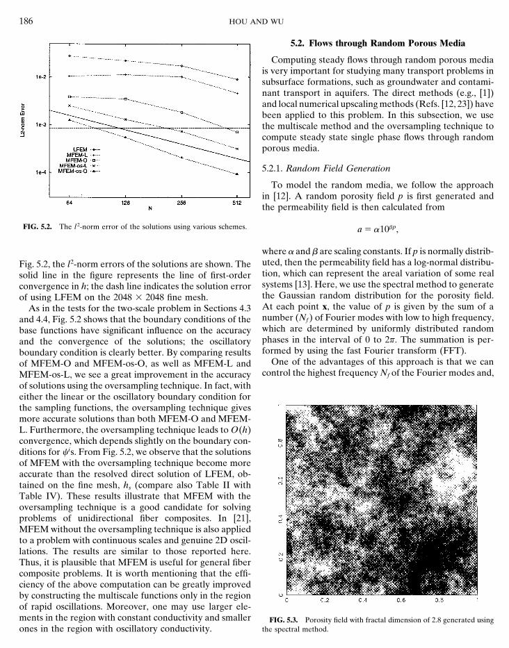
5.2.1. Random Field Generation

To model the random media, we follow the approachin [12]. A random porosity field p is first generated andthe permeability field is then calculated from

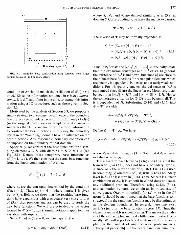
FIG. 5.2. The l 2-norm error of the solutions using various schemes. a 5 a10bp,

where a and b are scaling constants. If p is normally distrib-uted, then the permeability field has a log-normal distribu-Fig. 5.2, the l2-norm errors of the solutions are shown. Thetion, which can represent the areal variation of some realsolid line in the figure represents the line of first-ordersystems [13]. Here, we use the spectral method to generateconvergence in h; the dash line indicates the solution errorthe Gaussian random distribution for the porosity field.of using LFEM on the 2048 3 2048 fine mesh.At each point x, the value of p is given by the sum of aAs in the tests for the two-scale problem in Sections 4.3number (Nf ) of Fourier modes with low to high frequency,and 4.4, Fig. 5.2 shows that the boundary conditions of thewhich are determined by uniformly distributed randombase functions have significant influence on the accuracyphases in the interval of 0 to 2f. The summation is per-and the convergence of the solutions; the oscillatoryformed by using the fast Fourier transform (FFT).boundary condition is clearly better. By comparing results

One of the advantages of this approach is that we canof MFEM-O and MFEM-os-O, as well as MFEM-L andcontrol the highest frequency Nf of the Fourier modes and,MFEM-os-L, we see a great improvement in the accuracy

of solutions using the oversampling technique. In fact, witheither the linear or the oscillatory boundary condition forthe sampling functions, the oversampling technique givesmore accurate solutions than both MFEM-O and MFEM-L. Furthermore, the oversampling technique leads to O(h)convergence, which depends slightly on the boundary con-ditions for cis. From Fig. 5.2, we observe that the solutionsof MFEM with the oversampling technique become moreaccurate than the resolved direct solution of LFEM, ob-tained on the fine mesh, hs (compare also Table II withTable IV). These results illustrate that MFEM with theoversampling technique is a good candidate for solvingproblems of unidirectional fiber composites. In [21],MFEM without the oversampling technique is also appliedto a problem with continuous scales and genuine 2D oscil-lations. The results are similar to those reported here.Thus, it is plausible that MFEM is useful for general fibercomposite problems. It is worth mentioning that the effi-ciency of the above computation can be greatly improvedby constructing the multiscale functions only in the regionof rapid oscillations. Moreover, one may use larger ele-ments in the region with constant conductivity and smaller FIG. 5.3. Porosity field with fractal dimension of 2.8 generated using

the spectral method.ones in the region with oscillatory conductivity.

MULTISCALE FINITE ELEMENT METHOD 187

ratio between the maximum and minimum values of a(x) is400. We note that the permeability distribution is isotropic.The l2-norm errors obtained using various schemes areplotted in Fig. 5.4. In this case, the error of using MFEM-L increases initially as h decreases (N increases), which issimilar to the results shown in Section 4.3. This trend re-verses when h becomes smaller than the smallest scale ofthe problem, i.e., N 5 512. Again, the boundary conditionfor the base functions makes a big difference in the conver-gence trend. However, the influence in the accuracy is notas significant. The oversampling technique clearly im-proves both the accuracy and convergence. The rate ofconvergence of MFEM-os-O is lower than that computedin Fig. 5.2, about O(h0.2). Nevertheless, such a convergencebehavior is important in practice.

Next, in Fig. 5.5 we give the results for the fractal porosityfield shown in Fig. 5.3. The parameters of the simulation areFIG. 5.4. The l 2-norm error of the solutions using various schemesthe same as above. The fractal dimension 2.8 implies thatfor a log-normally distributed permeability field. The horizontal dash line

indicates the error of the LFEM solution with N 5 2048. the spectral energy density decays according to a (27/5)-power law. The decay of the small scales has a positiveeffect on the accuracy and convergence for all methods.

hence, the smallest scale contained in the porosity field. Among them, the oversampling technique still leads toThis control enables us to resolve the permeability field most accurate results. Note that the convergence rate ofby using a fine mesh. For example, given Nf 5 64, we may MFEM-os-O decreases as N increases. In fact, a similarchoose N 5 512 for the fine mesh. Then, there are five trend is also shown in the previous figure. In both cases,nodal points per shortest wavelength. Therefore, we may the errors of MFEM-os-O are very close to those of thecompute accurately resolved solutions for comparison with resolved LFEM solutions (the dash lines). The problemthe MFEM solutions. Another advantage of the spectral may be due to the effect of some residual layers that aremethod is that the power spectrum of the distribution can

not completely removed by the present implementation ofbe easily manipulated. This provides a convenient way ofthe oversampling technique. We will study this problemgenerating statistically fractal porosity distributions, whichin more detail in future works. On the other hand, we noteare found for many natural porous media [26]. More spe-that the MFEM with the oversampling technique is mostcifically, the spectral energy distribution of a statisticallyuseful in the unresolved regime where the oversamplingfractal field has a power-law structure. By constructing

random fields with different power-law spectrum, whichcan be easily done in the Fourier domain, one obtainsstatistically fractal fields with different fractal dimensions.For a detailed description about the correspondence be-tween the power law and the fractal dimension, we referto [26]. Because the random porosity fields used in oursimulations are very large, they have to be generated onthe parallel computer. A parallel FFT is developed for thispurpose. In addition, we use a parallel random numbergenerator described in [20] to generate the uniform devi-ates. A 256 3 256 image of a random porosity field withthe fractal dimension of 2.8 is shown in Fig. 5.3. In thefollowing, we solve (2.1) with u 5 0 on ­V and an uniformsource f 5 21. This is a model of flow in an oil reservoiror aquifer with uniform injection in the domain and outflowat the boundaries. As in Section 5.1, we fix N M 5 2048and choose MS 5 256.

5.2.2. ResultsFIG. 5.5. The l 2-norm error of the solutions using various schemes

First, we solve for a log-normal distribution of the per- for a fractally distributed permeability field. The horizontal dash lineindicates the error of the LFEM solution with N 5 2048.meability with Nf 5 256; a and b are chosen such that the

188 HOU AND WU

20482 mesh (the dash line). This is not surprising. We notethat the rapid oscillations in the vertical direction align withthe mesh. Therefore, the oscillatory boundary conditioncaptures the local property of the differential operator nearthe element boundaries. This makes the multiscale basefunctions very effective. For this reason, the oversamplingtechnique does not offer additional improved accuracyover the oscillatory boundary condition. The linear bound-ary condition, on the other hand, gives a poor convergenceresult since it cannot ‘‘sense’’ the layer structure. Thus itleads to the resonance effect, as shown in Fig. 5.7.

6. CONCLUDING REMARKS

We have successfully developed a multiscale finite ele-ment method for solving elliptic problems in compositematerials and porous media. The problems are character-ized by the highly heterogeneous and oscillatory coeffi-cients. In our method, the small scale information is cap-tured by the finite element bases constructed from theFIG. 5.6. Porosity field for cross section generated using the spec-leading order elliptic operator. In the case of periodic struc-tral method.ture, we prove that the method converges to the correcteffective solution as « R 0 independent of «. We have

technique performs well. The degeneration in the conver- analyzed the ‘‘resonant scale’’ phenomenon associatedgence rate should not be a big concern. with upscaling type of methods. To alleviate the difficulty,

We also note that the relative error of the LFEM solu- we propose an oversampling technique. Our numericaltion at N 5 512 is already less than 0.77%, which is small experiments give convincing evidence that the multiscaleenough for practical purposes. Thus, due to the decay of method is capable of capturing the large scale solutionsmall scales, one needs not resolve all the scales in order without resolving the small scale details. Applications ofto get satisfactory solutions. This observation should also the method to practical problems with continuous scalesbe applicable to MFEM. We use MFEM-os-O to compute seem promising. We demonstrate that at a reasonable cost,the problem with N 5 128 and M 5 4, which has an the multiscale method is able to solve very large scaleequivalent fine grid resolution as LFEM with N 5 512.The errors of the two solutions are rather close, 7.18 31024 for MFEM-os-O versus 6.86 3 1024 for LFEM.

In the previous two examples, the permeability fields areisotropic, which can model the areal variations of aquifers.However, the cross section of an aquifer is characterizedby the layer structures. Thus, the permeability field is aniso-tropic. In Fig. 5.6, the image of a numerically generatedporosity field for a cross section is shown. To generate thisfield, we let the Fourier modes decay in the x directionaccording to a given 1D fractal dimension (1.5 in our case),but the Fourier modes do not decay in the y direction.In this example, we have Nf 5 512 in the x direction andNf 5 256 in the y direction. The resulting distribution alongthe vertical direction for each fixed x is approximatelyGaussian. Thus, the permeability varies more rapidly alongthe vertical direction. For the permeability field, we choosea and b such that the ratio between the maximum andminimum values of a is 104.

The numerical errors are plotted in Fig. 5.7. We find FIG. 5.7. The l 2-norm error for cross section solutions using variousthat both MFEM-O and MFEM-os-O solutions have about methods. The horizontal dash line indicates the error of the LFEM solu-

tion with N 5 2048.the same accuracy as the resolved LFEM solution on the

MULTISCALE FINITE ELEMENT METHOD 189

11. J. E. Dendy, Jr. Black box multigrid, J. Comput. Phys., 48, 366 (1982).practical problems that are otherwise intractable using the12. L. J. Durlofsky. Numerical-calculation of equivalent grid block per-direct methods.

meability tensors for heterogeneous porous media, Water Resour.The idea of constructing multiscale base functions is notRes., 27, 699 (1991).

restricted to the elliptic equations. In the future, we will13. L. J. Durlofsky, Representation of grid block permeability in coarseapply the multiscale method to solve convection–diffusion scale models of randomly heterogeneous porous-media, Water Re-

equations and the wave equations in multiscale media. sour. Res., 28, 1791 (1992).Applications such as turbulent transport problems in high 14. B. B. Dykaar and P. K. Kitanidis, Determination of the effectiveReynolds number flows and wave propagation and scatter- hydraulic conductivity for heterogeneous porous media using a nu-

merical spectral approach: 1. method, Water Resour. Res., 28, 1155ing in random heterogeneous media will be considered.(1992).

15. W. E. and T. Y. Hou. Homogenization and convergence of the vortexACKNOWLEDGMENTSmethod for 2-d euler equations with oscillatory vorticity fields. Comm.Pure and Appl. Math., 43, 821 (1990).We thank Professor Bjorn Engquist and Mr. Yalchin Efendiev for

16. Y. Efendiev, T. Y. Hou, and X. H. Wu. A multiscale finite elementmany interesting and helpful discussions. This work is supported in partmethod for problems with highly oscillatory coefficients, in prepa-by ONR under the Grant N00014-94-0310 and DOE under the Grantration.DE-FG03-89ER25073.

17. B. Engquist and T. Y. Hou. Particle method approximation of oscilla-tory solutions to hyperbolic differential equations. SIAM J. Numer.REFERENCESAnal., 26, 289 (1989).

18. B. Engquist and E. Luo. Multigrid methods for differential equations1. R. Ababou, D. McLaughlin, and L. W. Gelhar, Numerical simulationwith highly oscillatory coefficients, In Proceedings of the Sixth Copperof three-dimensional saturated flow in randomly heterogeneous po-Mountain Conference on Multigrid Method, 1993.rous media, Transport in Porous Media 4, 549 (1989).

19. J. Frehse and R. Rannacher. Eine l1-fehlerabschatzung fur diskrete2. M. Avellaneda, T. Y. Hou, and G. Papanicolaou, Finite differenceGrundlosungen in der Methode der finiten Elemente, In Finiteapproximations for partial differential equations with rapidly oscillat-Elemente, No. 89, edited by J. Frehse (Bonn. Math. Schrift., Bonn,ing coefficients, Math. Modelling Numer. Anal. 25, 693 (1991).1975), p. 92.3. M. Avellaneda and F-H. Lin, Homogenization of elliptic problems

20. B. L. Holian, O. E. Percus, T. T. Warnock, and P. A. Whitlock,with Lp boundary data, Appl. Math. Optim. 15, 93 (1987).Pseudorandom number generator for massively-parallel molecular-4. I. Babuska, G. Caloz, and E. Osborn, Special finite element methodsdynamics simulations, Phys. Rev. E 50(2), 1607 (1994).for a class of second order elliptic problems with rough coefficients,

21. T. Y. Hou, X. H. Wu, and Z. Cai, Convergence of a multiscaleSIAM J. Numer. Anal. 31, 945 (1994).finite element method for elliptic problems with rapidly oscillating5. I. Babuska and E. Osborn, Generalized finite element methods: Theircoefficients, Math. Comput., submitted.performance and their relation to mixed methods, SIAM J. Numer.

22. P. Jussel, F. Stauffer, and T. Dracos. Transport modeling in heteroge-Anal. 20, 510 (1983).neous aquifers. 2. 3-dimensional transport model and stochastic nu-6. I. Babuska and W. G. Szymczak, An error analysis for the finitemerical tracer experiments. Water Resour. Res., 30, 1819 (1994).element method applied to convection-diffusion problems, Comput.

23. J. F. McCarthy. Comparison of fast algorithms for estimating large-Methods Appl. Math. Engrg. 31, 19 (1982).scale permeabilities of heterogeneous media. Transport in Porous7. J. Bear. Use of models in decision making, in Transport and ReactiveMedia, 19, 123 (1995).Processes in Aquifers, edited by T. H. Dracos and F. Stauffer (Bal-

24. R. Scott. Optimal l y estimates for the finite element method onkema, Rotterdam, 1994), p. 3.irregular meshes. Math. Comput. 30, 681 (1976).8. A. Bensoussan, J. L. Lion, and G. Papanicolaou, Asymptotic Analysis

25. A. F. B. Tompson. Numerical-simulation of chemical migration infor Periodic Structure, Studies in Mathematics and Its Applications,physically and chemically heterogeneous porous-media. Water Re-Vol. 5 (North-Holland, Amsterdam, 1978).sour. Res., 29, 3709 (1993).9. D. T. Burr, E. A. Sudicky, and R. L. Naff, Nonreactive and reactive

26. D. L. Turcote and J. Huang. Fractal distributions in geology, scalesolute transport in 3-dimensional heterogeneous porous media—invariance, and deterministic chaos. In C. C. Barton and P. R. Lamean displacement, plume spreading, and uncertainty, Water Resour.Pointe, editors, Fractals in the Earth Sciences, pages 1–40. PlenumRes., 30, 791 (1994).Press, 1995.10. M. E. Cruz and A. Petera, A parallel Monte-Carlo finite-element

procedure for the analysis of multicomponent random media, Int. J. 27. P. M. De Zeeuw. Matrix-dependent prolongation and restrictions ina blackbox multigrid solver. J. Comput. Applied Math., 33, 1 (1990).Numer. Methods Eng. 38, 1087 (1995).