A Multidisciplinary Optimization Framework for Control

A Multidisciplinary Optimization Framework

for Control-Configuration Integration in

Aircraft Conceptual Design

Ruben E. Perez∗ and Hugh H. T. Liu†

University of Toronto, Toronto, ON, M3H 5T6, Canada

Kamran Behdinan‡

Ryerson University, Toronto, ON, M5B 2K3, Canada

The emerging flight-by-wire and flight-by-light technologies increase the

possibility of enabling and improving aircraft design with excellent han-

dling qualities and performance across the flight envelope. As a result,

it is desired to take into account the dynamic characteristics and auto-

matic control capabilities at the early conceptual stage. In this paper,

an integrated control-configured aircraft design sizing framework is pre-

sented. It makes use of multidisciplinary design optimization to overcome

the challenges which the flight dynamics and control integration present

when included with the traditional disciplines in an aircraft sizing process.

A commercial aircraft design example demonstrates the capability of the

proposed methodology. The approach brings higher freedom in design,

leading to aircraft that exploit the benefits of control configuration. It also

helps to reduce time and cost in the engineering development cycle.

Nomenclature

c mean aerodynamic chord, ft

r reference signal

u control vector

∗Ph.D. Candidate, Institute for Aerospace Studies, and AIAA Student Member†Associate Professor, Institute for Aerospace Studies, and AIAA Member‡Associate Professor and Chair, Department of Aerospace Engineering, and AIAA Member

1 of 29

x state vector

y output vector

A state matrix

AR aspect ratio

B input matrix

C output matrix

c chord length, ft

CD drag coefficient

CL lift coefficient

ESF engine scaling factor

f objective function

HQL handling quality level

Iyy pitching moment of inertia, slug-ft2

J compatibility constraint

K feedback control gain

M pitch moment

MTOW maximum takeoff weight, lb

nz normal acceleration, g’s/rad

p roll rate, deg/sec

q pitch rate, rad/sec

r yaw rate, deg/sec

S area, ft2

T engine thrust, lb

tpk response peak time, sec

tc thickness to chord ratio

TSFC thrust specific fuel consumption

V aircraft velocity, ft/sec

x local design variable

y coupling design variable

Z normal force

z global design variable

Subscripts

a aileron

ce control effector

cs control surface

dr dutch roll

e elevator

2 of 29

eng engine

ht horizontal tail

i ith discipline

ic inner chord

oc outer chord

r rudder

ref reference value

SL system level

sp short period mode

vt vertical tail

w wing

wo washout filter

Symbols

α angle of attack, rad

β sideslip angle, deg

δ deflection, deg

η normalized control effector span location

Λ sweep angle, deg

λ taper ratio

ω frequency, rad/sec

φ bank angle, deg

τ time constant

ε constraint tolerance value

ζ damping ratio

I. Introduction

Flight dynamics and control (FD&C) has a significant impact on the aircraft performance

and cost.1 It is also an important discipline for flight safety and aircraft certification. Con-

siderations of dynamic characteristics and control design are essential in the design of future

aircraft. Furthermore, the use of control-augmented or control-configured vehicles could offer

significant opportunities for expanded flight envelopes and enhanced performance, as demon-

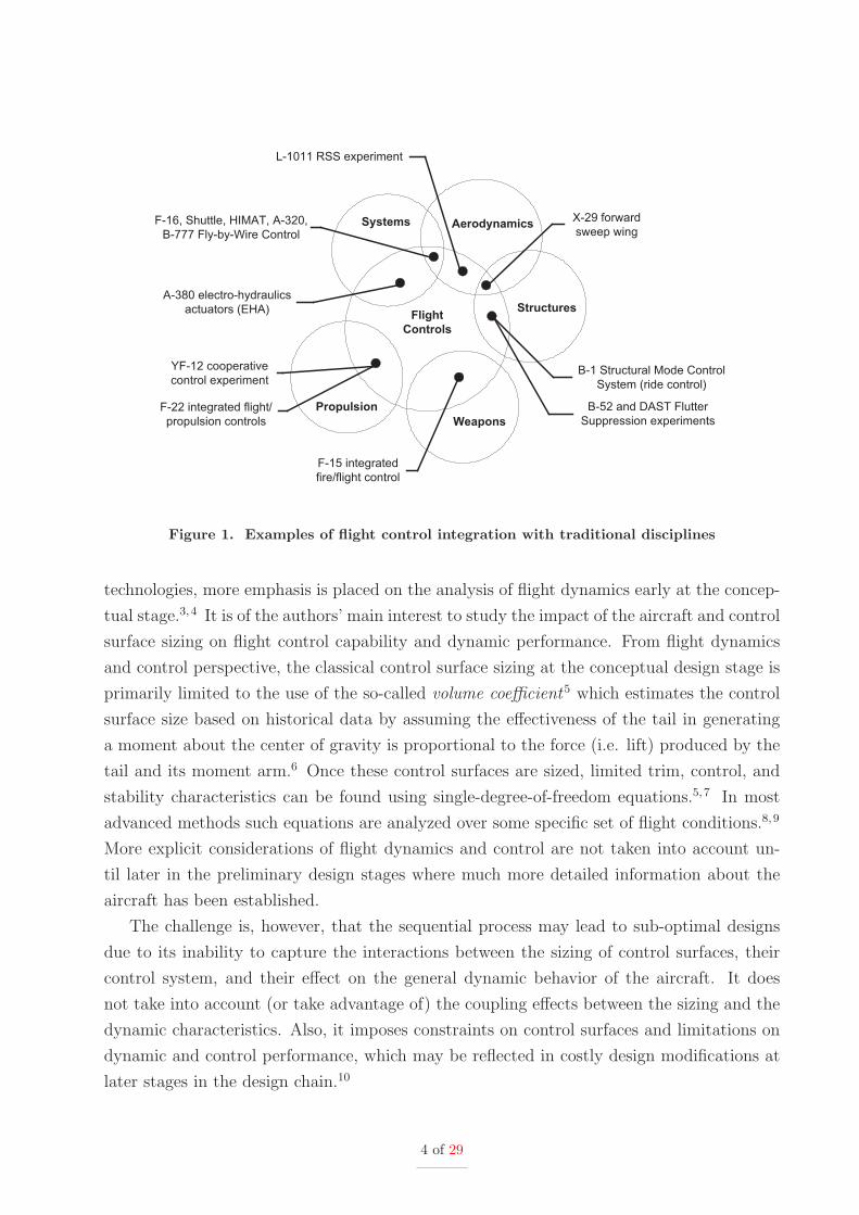
strated over the years with different research efforts as shown in Figure 1 adapted from Ref. 2.

In the traditional conceptual design process, the disciplinary analyses are performed se-

quentially. It is an iterative process in which interdisciplinary trades are used to size the

aircraft. With the advances of new technologies such as flight-by-wire and flight-by-light

3 of 29

Aerodynamics

Structures

Weapons

Flight

Controls

Systems

Propulsion

B-1 Structural Mode Control

System (ride control)

F-15 integrated

fire/flight control

YF-12 cooperative

control experiment

F-22 integrated flight/

propulsion controls

A-380 electro-hydraulics

actuators (EHA)

X-29 forward

sweep wing

B-52 and DAST Flutter

Suppression experiments

F-16, Shuttle, HIMAT, A-320,

B-777 Fly-by-Wire Control

L-1011 RSS experiment

Figure 1. Examples of flight control integration with traditional disciplines

technologies, more emphasis is placed on the analysis of flight dynamics early at the concep-

tual stage.3,4 It is of the authors’ main interest to study the impact of the aircraft and control

surface sizing on flight control capability and dynamic performance. From flight dynamics

and control perspective, the classical control surface sizing at the conceptual design stage is

primarily limited to the use of the so-called volume coefficient5 which estimates the control

surface size based on historical data by assuming the effectiveness of the tail in generating

a moment about the center of gravity is proportional to the force (i.e. lift) produced by the

tail and its moment arm.6 Once these control surfaces are sized, limited trim, control, and

stability characteristics can be found using single-degree-of-freedom equations.5,7 In most

advanced methods such equations are analyzed over some specific set of flight conditions.8,9

More explicit considerations of flight dynamics and control are not taken into account un-

til later in the preliminary design stages where much more detailed information about the

aircraft has been established.

The challenge is, however, that the sequential process may lead to sub-optimal designs

due to its inability to capture the interactions between the sizing of control surfaces, their

control system, and their effect on the general dynamic behavior of the aircraft. It does

not take into account (or take advantage of) the coupling effects between the sizing and the

dynamic characteristics. Also, it imposes constraints on control surfaces and limitations on

dynamic and control performance, which may be reflected in costly design modifications at

later stages in the design chain.10

4 of 29

In order to address this challenge, a noval method for the concurrent design of the con-

trol system and the aircraft, including the control surface sizing, is presented in this paper.

Using a multidisciplinary design optimization (MDO) approach, the control surface sizing

with feedback flight control system development is integrated in the conceptual aircraft siz-

ing process. Because more disciplinary aspects of the aircraft are considered simultaneously,

better control-augmented aircraft designs can be obtained, based on specified mission pa-

rameters, including flight dynamics, handling quality and control related objectives over the

entire aircraft mission profile.

II. Integration Methodology Challenges

While the benefits of simultaneous considerations of flight dynamics and control in aircraft

design have been considered since the 1970s,11 very few efforts have been made over the years

to integrate FD&C in the conceptual design phases. A number of challenges are given below.

First of all, the aircraft design has to guarantee satisfactory flight characteristics over the

entire flight envelope. In order to ensure positive characteristics, proper control is required

for each point within the envelope. The number of analyses required to cover the entire

envelope becomes unaffordable at the conceptual stage.

Second, unlike many other disciplines involved in the conceptual design process, FD&C

does not have an obvious figure-of-merit (FOM) that can be used for design optimization. For

example, drag count is a continuous FOM used in aerodynamics where the disciplinary goal

is to minimize such measurement. The challenge lies in the proper specification definition

that considers the dynamics and control requirements and constraints simultaneously.

Third, in the current design process very few interactions between the control and aircraft

design processes are taken into account. As a result, when the design has been frozen and

information regarding the design matures, so better disciplinary information is known, any

deficiencies in FD&C which could be avoided by considering such interactions suddenly

become very expensive to fix; as they requires changes to control surfaces, additional wind

tunnel testing to place vortex generators, installation of redundant control systems, etc. The

challenge lies in how to enable control-configuration interactions at the conceptual design

stage not only to exploit the coupling benefits that arise from such integration but also to

reduce any possible FD&C deficiencies as early as possible.

A final obstacle is how to deal with the increased data and computational complexity.

5 of 29

III. Flight Dynamics and Control Integration Methodology

The proposed methodology makes use of multidisciplinary optimization to solve the de-

sign complexity paradigm while simultaneously designing the aircraft and the control system

at different constraining conditions. Details of the proposed solution to flight dynamic and

control integration challenges are presented in the following subsections.

A. Multidisciplinary Design Integration

With recent advances in the field of multidisciplinary optimization (MDO),12 it is possi-

ble to transform the traditional vertical design process into a horizontal process, enabling

concurrent analysis and design. Therefore, it is possible to address the FD&C integra-

tion/interaction challenge, and take advantage of the concurrent structure to increase free-

dom in the design space. Among many different MDO strategies, Collaborative Optimization

(CO)13 shown in Figure 2 has been found to be one suitable alternative to include flight dy-

namics and control in the design process. CO is a bi-level optimization scheme that decouples

the design process by providing the common design variables and disciplinary coupling in-

teractions all at once in an upper level, eliminating the need for an a priori process that

accumulates all the disciplinary data required to perform FD&C analyses.

System Level Optimizer

Goal: Design Objective

s.t. Interdisciplinary

Compatibility Constraints

Disciplinary Optimizer 1

Goal: InterdisciplinaryCompatibility

s.t. Disciplinary

Constraints


Goal: Interdisciplinary

Compatibility

s.t. Disciplinary

Constraints


Goal: Interdisciplinary

Compatibility

s.t. Disciplinary

Constraints

Analysis 1 Analysis 2 Analysis 3

Figure 2. Collaborative Optimization Method

At the system-level (SL), the Collaborative Optimization objective function is stated as:

minzSL,ySL

f (zSL, ySL)

s.t. J∗i

(

zSL, z∗i , ySL, y∗i

(

x∗i , y

∗j , z

∗i

))

≤ ε i, j = 1, ..., n j 6= i(1)

where f represents the system level objective function. J∗i represents the compatibility

6 of 29

constraint for the ith subsystem (of the total n subsystems) optimization problem, and ε is a

constraint tolerance value. Variables shared by all subsystems are defined as global variables

(z). Variables calculated by a subsystem and required by another are defined as coupling

variables (y). Variables with superscript star indicate optimal values for the subsystem level

optimization. Note that the system level constraint assures simultaneous coordination of the

coupled disciplinary values. When using local optimization schemes the MDO mathematical

foundation leads to a unique ‘multidisciplinary feasible point’, which is the optimal solution

for all disciplines.

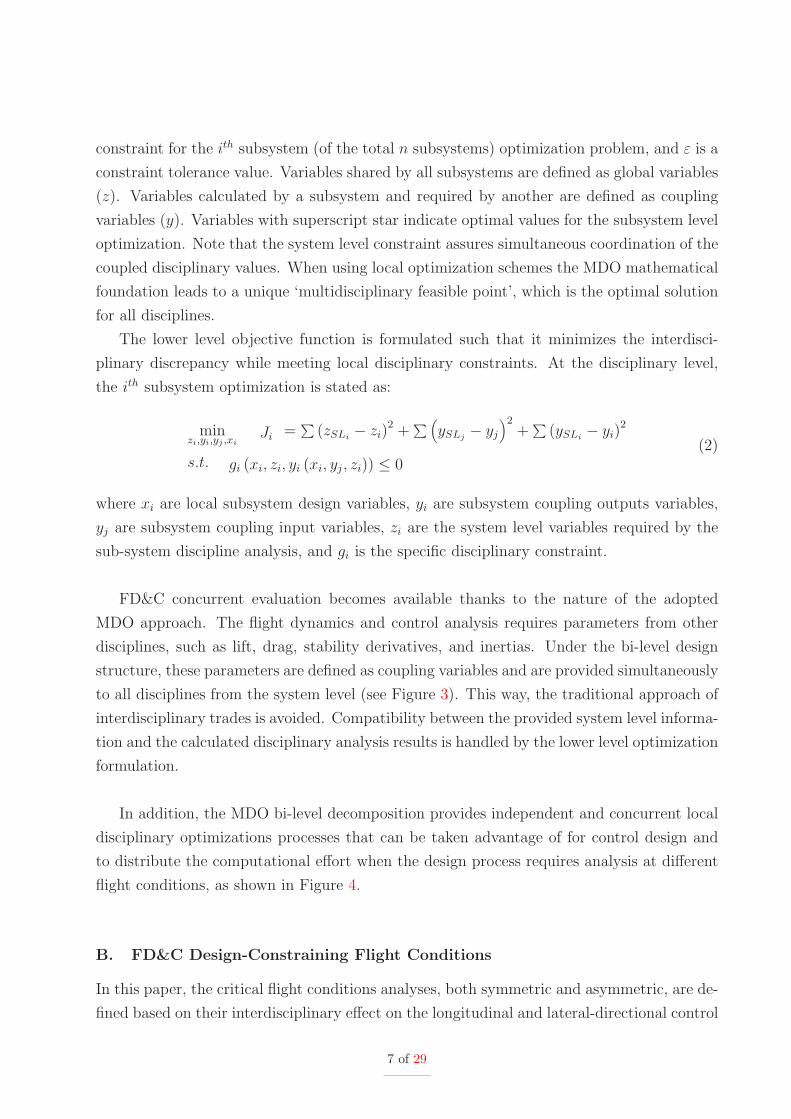
The lower level objective function is formulated such that it minimizes the interdisci-

plinary discrepancy while meeting local disciplinary constraints. At the disciplinary level,

the ith subsystem optimization is stated as:

minzi,yi,yj ,xi

Ji =∑

(zSLi− zi)

2 +∑

(

ySLj− yj

)2+

∑

(ySLi− yi)

2

s.t. gi (xi, zi, yi (xi, yj, zi)) ≤ 0(2)

where xi are local subsystem design variables, yi are subsystem coupling outputs variables,

yj are subsystem coupling input variables, zi are the system level variables required by the

sub-system discipline analysis, and gi is the specific disciplinary constraint.

FD&C concurrent evaluation becomes available thanks to the nature of the adopted

MDO approach. The flight dynamics and control analysis requires parameters from other

disciplines, such as lift, drag, stability derivatives, and inertias. Under the bi-level design

structure, these parameters are defined as coupling variables and are provided simultaneously

to all disciplines from the system level (see Figure 3). This way, the traditional approach of

interdisciplinary trades is avoided. Compatibility between the provided system level informa-

tion and the calculated disciplinary analysis results is handled by the lower level optimization

formulation.

In addition, the MDO bi-level decomposition provides independent and concurrent local

disciplinary optimizations processes that can be taken advantage of for control design and

to distribute the computational effort when the design process requires analysis at different

flight conditions, as shown in Figure 4.

B. FD&C Design-Constraining Flight Conditions

In this paper, the critical flight conditions analyses, both symmetric and asymmetric, are de-

fined based on their interdisciplinary effect on the longitudinal and lateral-directional control

7 of 29

PropDesign

StructDesign

Aero

Design

Airplane

Config

PerfDesign

Optimization

Inter- Disciplinary

Trades

FlightDynamics

ControlDesign

Weights

& Balance

(a) Traditional Design Process (Vertical Develop-ment)

Prop

Design

Struct

Design

Aero

Design

Perf

Design

FlightDynamics&

Control

Optimization

Disciplinary DataAircraft Configuration

Weights

& Balance

(b) MDO Design Process (Horizontal Developmentdue to Variable Decoupling)

Figure 3. Flight Dynamics and Control Decoupling

WeightsOptimizer

Weights Aerodynamics

PerformanceOptimizer

AerodynamicOptimizer

Performance

System Level

Optimizer

FD & Control

FD & ControlOptimizer

Aerodynamics



Performance FD & Control


Aerodynamics



Performance FD & Control


Takeoff Cruise Approach & Landing

Takeoff

Cruise

Approach & Landing

...

Climb

Loiter

Diversion

Figure 4. Mission Segments Disciplinary Decomposition

8 of 29

surfaces sizing as presented in Table 1. They contain static, maneuver, inertia coupling and

dynamic considerations along the flight envelope and are valid for a large range of aircraft

configuration and concepts.8,14–16 Only primary design conditions are considered. Critical

control failure cases are neglected since they represent secondary requirements and can be

covered in great extent by open-loop and closed-loop dynamic requirements.

Table 1. Longitudinal and Lateral-Directional Design-Constraining Conditions

Control EffectorAnalysis

Applicable FlightConditions

Critical CGLocation

ApplicableRequirement

Aircraft Configuration

Longitudinal

1-g Trim All Fwd, Aft FAR/JAR 25.161C Dependent on Flight Condition

Approach 1-g Trim Approach Fwd FAR/JAR 25.161C Full Flaps

Landing 1-g Trim Landing Fwd FAR/JAR 25.161C Full Flaps, Landing Gear Down

Go-Around 1-g Trim Climb Aft FAR/JAR 25.161C Full Flaps, Landing Gear Down

Manoeuvre Load All Fwd FAR/JAR 25.255 Dependent on Flight Condition

Go-Around maneuver Approach Fwd FAR/JAR 25.255 Full Flaps

Rotation on Takeoff Takeoff Fwd FAR/JAR 25.143 Takeoff Flaps, Landing GearDown, in ground effect

Rotation on Landing Landing Aft FAR/JAR 25.143 Full Flaps, Landing Gear Down,in ground effect

Dynamic Mode Oscillation All Fwd, Aft FAR/JAR 25.181A Dependent on Flight Condition

Lateral

Steady Sideslip All - FAR/JAR 25.177 Dependent of Flight Condition

One Engine InoperativeTrim

All - FAR/JAR 25.161 Dependent of Flight Condition

Time to Bank All - FAR/JAR 25.147 Dependent of Flight Condition

Inertia Coupling (Pitchdue to Velocity Axis Roll)

Cruise - FAR/JAR 25.143 Dependent of Flight Condition

Yaw Due to Loaded RollPullout


Coordinated Velocity AxisRoll


Dutch Roll Oscillation All - FAR/JAR 25.181B Dependent of Flight Condition

Roll Subsidence All - FAR/JAR 25.181B Dependent of Flight Condition

Spiral Divergence All - FAR/JAR 25.181B Dependent of Flight Condition

Closed-Loop Stability All - FAR/JAR 25.177 Dependent of Flight Condition

Longitudinal static considerations are aimed to maintain steady 1-g level flight, which can

become highly demanding for the control effectors at low speeds in both forward (fwd) and

aftward (aft) CG limits, and with complex high lift devices (where the aerodynamic pitching

moment is large) as is the case in the approach and go-around flight phases. Maneuver

considerations include load and rotation capabilities. In the first one the control effectors

should be able to achieve load factors between the maximum and minimum operational lim-

its in a pull-up from a dive over the flight envelope. This scenario becomes critical with the

maximum takeoff weight and fwd CG, and in the go-around maneuver where the control

effectors should be able to provide 8 deg/sec2 pitch acceleration starting from an approach

trim condition. Rotation capabilities consider the ability of the control effectors to gener-

9 of 29

ate enough pitch moment to lift/de-rotate the nose wheel off/on the ground in takeoff and

landing respectively. This scenario becomes critical for takeoff at maximum gross weight

with fwd CG, and with complex high-lift systems and high CG locations for landing. A

pitch acceleration of 7 deg/sec2 for dry, prepared runways is specified for takeoff, it is higher

than the minimum requirement as specified by FAR 25.331C, to provide an ample margin

of control for future aircraft variants. Longitudinal dynamic response considerations are in-

cluded as well for both the un-augmented (open-loop) and augmented (closed loop) aircraft.

With a control-augmented aircraft the closed-loop dynamic criteria assessment serves pri-

marily for the evaluation of control laws. However, consideration of these conditions during

the conceptual sizing stage ensures the aircraft is properly designed for adequate dynamic

characteristics where control-augmentation is used to avoid excessive system demands.

For the lateral-directional dynamics, the static considerations include steady sideslip

and one-engine-inoperative (OEI) considerations. For the steady sideslip the lateral control

surfaces should provide adequate roll and yaw power to perform steady sideslip maneuver at

a 10-degree sideslip angle. This situation becomes critical during crosswind landing, when

the sideslip angle is the greatest because of low airspeed. Similarly, the roll and yaw control

effectors must be able to cope with asymmetric propulsion failure and maintain a steady

straight flight with a 5 degree bank angle. This requirement becomes most demanding when

operating at very low speed, specifically at takeoff where the weight and inertia are higher.

A lateral-directional dynamic consideration is related to the time to bank response to full roll

control input where the maneuver result must meet the performance requirements prescribed

by Ref. 17. Similar to the longitudinal case, critical dynamic characteristics are considered

where the dynamic mode response for both the un-augmented (open-loop) and augmented

(closed loop) aircraft is assessed.

Three inertia coupling effects are included as well. The first one considers the pitch due to

velocity axis roll, where the control effectors (elevators) should provide sufficient nose-down

pitch authority to compensate for the nose-up moment as a result of inertia cross-coupling

during high angle-of-attack stability axis roll maneuvers. Similarly, the control effectors

(rudder) should possess adequate authority to overcome the yawing moment as a result

of inertia coupling during a rolling pullout maneuver. In addition, the control effectors

(rudder and ailerons) should be able to maintain a zero sideslip conditions when performing

a coordinated stability-axis roll.

Note that many of the above critical conditions for the control effectors match the tradi-

tional design mission profile flight phases which greatly simplify the flight condition analyses.

However, if necessary other off-mission design conditions can be calculated and taken into

consideration in the design process.

10 of 29

C. FD&C Design Constraints and Requirements

Control power, which describes the efficiency of a control system in producing a range of

steady equilibrium or maneuvering states18 is defined as the common figure-of-merit to be

used in FD&C. It is quantified in terms of control deflection making it a continuous measure-

ment useful for optimization. Specific sets of flight condition analyses will become critical, as

the aircraft geometry varies during sizing. To ensure adequate flight control characteristics,

the aircraft has to provide sufficient, yet not excessive, control power to meet the require-

ments of the prescribed flight analyses. For such reason, the FD&C disciplinary constraints

in 2 are specified in terms of such FOM, along with complementary open and closed loop

dynamic requirements. The additional open-loop constraints take care of dynamic response

specifications, such as limits of oscillation, damping ratios, natural frequency requirements,

and control force gradients, which are defined from military specifications (such as Ref. 17),

or certification guidelines (such as FAR or JAR). The closed-loop constraints are mainly

aimed to meet with control design requirements in order to achieve internal stability of the

control system, reject external disturbances, and assure adequate handling qualities (HQ)

requirements for both the longitudinal and lateral-directional modes. The assessment of HQ

is closely related to dynamic considerations of the augmented closed-loop aircraft. Different

handling qualities quantification procedures exist. For the longitudinal case, the method

such as the one proposed in Ref. 19 is very useful for an optimization procedure. It directly

quantifies dynamic modes responses with HQ.

For example, if the aircraft dynamics is considered to be uncoupled into longitudinal and

lateral modes, the short period mode handling quality can be assessed by using a control

anticipation parameter (CAP). This parameter quantifies the response necessary to make

precise adjustments to the flight path in terms of instantaneous angular pitching accelera-

tion per unit of steady state normal acceleration.20 Furthermore, a generic control antici-

pation parameter (GCAP) extends the CAP application to both un-augmented and control

augmented aircraft.21 The GCAP parameter is defined as:

GCAP = q(0)

nz(tpk)

(

1 + exp(

−ζspπ√1−ζ2

sp

))

0 < ζsp < 1(3)

where nz(tpk) is the normal acceleration at the peak time in response to a control step

input. Specified GCAP bounds correlate the qualitative HQ levels to the aircraft step input

dynamic response. In the case of the Phugoid mode, handling quality is related to the mode

damping and time to double amplitude to ensure long enough time to stabilize the aircraft

following a disturbance. Lateral HQ include roll and bank oscillations responses, a sideslip

excursion and a ‘Phi-to-Beta’ (φ/β) ratio criteria specifications.17,19

11 of 29

D. Control System Design

While some research has been done to select the most appropriate control system at the

design stage before any detailed analysis is performed (see e.g. Ref. 22), the proposed

methods do not perform the actual control design, therefore limiting their capability in

the scope of control-configured aircraft design. Among the different control systems, the

stability augmentation systems (SAS) have the strongest relationship with the design of

the airplane, since their use can directly affect the aircraft layout characteristics. For this

reason the control design goal at the conceptual design stage is to provide adequate stability

augmentation systems to meet the close-loop and handling quality specifications over the

flight envelope for both longitudinal and lateral dynamics. The aircraft plant is defined as a

strictly proper linear time invariant (LTI) system without disturbances and sensor noise. An

output feedback controller, Figure 5, is used to provide the necessary stability augmentation.

The feedback control is formulated as:

˙x = Ax + Bu

y = Cx

u = r − Ky

where : K =

k11 . . . k1d

.... . .

...

kc1 . . . kcd

(4)

where x is the aircraft states, y is the plant output, u is the control variables, r is the

reference signal, c is the number of control variables u, and d is the number of outputs y,

and A,B,C are the state, control and output matrices respectively. The closed-loop system

is then:

y = C (sI − Ac)−1 Br

where : Ac = A − BKC(5)

Plant

K

u y+

-r

Figure 5. Generalized Control Process

Stability is assured by selecting adequate control gains such that the closed loop system

12 of 29

lies in the negative real axis. It is assumed the aircraft dynamics follow “traditional” mode

responses for both longitudinal and lateral dynamics so the sign of the gains can be selected

beforehand to guarantee stabilization. The control design itself is done as part of the MDO

lower-level optimization, where control gains are specified as local optimization variables

x in (2), while closed-loop stability and control constraints assure proper stabilization and

performance.

IV. Application Example

A. Aircraft Mission and Optimization Goal

This section illustrates the proposed framework process in the case of a narrow-body 130-

passenger airliner sizing, with twin wing engines, and conventional aft tail. Its mission profile

is specified in Figure 6, in line with industry standards for similarly sized aircraft. The design

goal (MDO system level goal, eq. (1)) is to find a feasible aircraft that maximizes specific

air range ( maxzSL,ySL

Range ) while meeting individual disciplinary requirements as shown in

the mission profile. A fixed fuel weight is specified as 40000 lb, while the payload weight is

specified as 32175 lb based on 130 passengers, crew of 2, and 5 attendants. The subsystem

level disciplinary optimization process follow the formulation presented in eq. (2).

Start Engine, Warm up & Taxi,

Takeoff within 5500 ft

CEA: 1, 6, 10, 11

Climb II

G > 0.024

Climb / Accelerate

CEA: 1, 4, 8, 9, 10,

11, 12, 16, 17

max. Cruise

(35000 ft) – Mach 0.78

CEA: 1, 4, 8, 9, 10, 11,

12, 13, 14, 15, 16, 17

Loiter 30 min.

1500 ft

Missed Approach

G > 0.024

CEA: 3, 5, 8, 9,

10, 11, 12, 16, 17

Descend & Land

within 5000 ft

CEA: 1, 7, 10, 11

Approach

CEA: 1, 2, 4, 8,

9, 10, 12, 16, 17

Control Effector Analysis (CEA)

Longitudinal CEA

1 – Longitudinal Trim

2 – Approach Trim

3 – Go-Around Trim

4 – Maneuver Load

5 – Go-Around Maneuver Load

6 – Takeoff Rotation Power

7 – Landing Rotation Power

8 – Longitudinal Modes Response

9 – Longitudinal Handling Qualities

Lateral CEA

10 – Steady Sideslip

11 – One Engine Inoperative Trim

12 – Time to Bank

13 – Pitch due to velocity axis roll

14 – Yaw due to Loaded Roll Pullout

15 – Coordinated Velocity Axis Roll

16 – Lateral Modes Response

17 – Lateral Handling Qualities

Diversion

200 nm - (25000 ft)

Mach 0.78

Remarks:

- Reserves include 5% flight fuel contingency.

- Takeoff and landing, sea level, ISA, no wind.

Figure 6. Mission Profile and Longitudinal Control Effectors Analysis Considered

B. Disciplinary Analyses

The design process of this example is composed of five coupled disciplines, namely: weights,

aerodynamics, propulsion, performance, and dynamics & control. They are coupled as shown

13 of 29

in the n-square diagram presented in Figure 7. Details of each discipline are described below.

Weights

Aerodynamics

Performance

Dynamics

& Control

Aircraft

Layout

Propulsion

Figure 7. Design Example Disciplinary Couplings

• Weights: The aircraft takeoff weight is calculated from main component weights that

are estimated using statistical methods.6,23 The maximum permissible center of gravity

(CG) range for the configuration is calculated from each aircraft component permissible

CG limits, based on their own geometry, physical and functional considerations.24

Similarly, the aircraft inertias are calculated from a build-up based on each component

inertias calculated from the mean CG location for each component.

• Aerodynamics: Aircraft lift, drag and stability derivatives are calculated based on stan-

dard aerodynamic calculation used at the conceptual stage. Induced, parasite and wave

drag calculations are considered. The induced drag is calculated from parametric tech-

nology models whereas parasite-drag is calculated using a detailed component build-

up25 taking into consideration viscous separation and components mutual interference

effects. Transonic wave drag is modeled based on Lock’s empirical approximation,

using the Korn equation extended by Mason to include sweep.26 To provide greater

flexibility and accuracy in the calculation of aerodynamic characteristics, downwash

effects, and stability derivatives, a combination of semi-empirical formulae27,28 and a

non-planar multiple lifting surface panel method are implemented.

• Performance: Takeoff and landing distances, rate of climb, and range are calculated

based either on analytical expressions or numerical simulations. For example, take-

off distance is calculated based on a numerical simulation, while specific air range is

14 of 29

calculated based on Breguet’s equation. Landing field length is calculated assuming a

landing weight of 90% MTOW.

• Propulsion: Propulsion characteristics, such as engine weight, thrust and specific fuel

consumption for a given altitude and Mach number, are calculated based on engine

scaling of a baseline PW-2037 high bypass turbofan engine.

• Flight Dynamics and Control: For the present analysis it is assumed that all aircraft

states are measurable without noise. Longitudinal and lateral design open-loop, and

closed-loop analyses are performed at each flight mission segment as shown on Figure 6.

Control design is performed for all in-flight phases (climb, cruise, and landing approach)

of the mission profile.

C. Control Systems Design

In this example, the stability augmentation system uses standard cascaded SISO gains for

the longitudinal and lateral-directional modes as shown in Figure 8.

Aircraft

Ka

Kq

Kb

Kr

Kp

+-

+-

+-

δaf

δef

δrf

δec

δac

δrc

rf

α

q

p

r

β

Washout Filter

s/s wo+1τ

Figure 8. Designed Stability Augmentation System

Longitudinal Stability Augmentation

Among the longitudinal modes the short period response is of prime concern due to its

rapid response and its correlation with handling qualities evaluation. For this reason, efforts

15 of 29

are concentrated in designing the stability augmentation system (SAS) of this mode. The

longitudinal short period flight dynamics equations can be formulated as:29

α

q

=

Zα/V 1

Mα + MαZα/V Mq + Mα

α

q

+

Zα/V

Mδ + MαZδ/V

[δe] (6)

where α and q are the angle of attack and pitch rate respectively,[

Mα Zα Mα Mq

]

and[

MδeZδe

]

are the dimentional stability derivatives and control derivatives respectively;

their formulation include the inertia terms, i.e. Mα =qSref c

Iyy

∂Cm

∂α.

Every dynamic state is affected by the elevator deflection control input signal. The control

system is designed to achieve Level I handling qualities performance while meeting natural

damping and frequency limit characteristics. The output feedback gains can be expressed

as:

{u} = δe = δer−

[

kα kq

]

α

q

(7)

Lateral-Directional Stability Augmentation

The lateral flight control system provides lateral/directional stabilization. It consists of a roll

feedback and yaw damper implemented to improve the Dutch roll damping. The washout

filter time constant in the yaw damper depends on the washout corner frequency ωwo as:

1

τwo

= ωwo = kwoωndr(8)

where kwo is a control design variable representing a percentage of the Dutch roll natural

frequency value.

The open-loop lateral dynamics equations are omitted but they follow the standard LTI

form state space form given as: { ˙x} = [A] {x} + [B] {u} where {x} =[

β p φ r

]T

and

{u} =[

δa δr

]T

. The lateral output feedback gains can be expressed as:

{u} =[

δa δr

]T

=[

δa δr

]T

r−

0

−krωwo

x5 +

0 kp 0 0

kβ 0 0 krωwo

β

p

φ

r

(9)

where x5 is an additional state that arise from the inclusion of the washout filter in the

16 of 29

state space representation. Note that as described in III, the closed loop system stability is

guaranteed by selecting adequate control gain direction and values.

D. Design Variables and Constraints

Table 2 lists the design variables and their bounds used for the optimization. At the system

level, 102 design variables are taken into consideration, from which 18 are global design vari-

ables and 84 are coupling design variables. The global design variables specify the general

aircraft geometric configuration. Coupling variables include four flight condition independent

terms (engine scaling factor, MTOW, fuel and engine weights), while the rest are distributed

over the different flight conditions. Local variables are specified only to the flight dynamic

and control discipline and correspond to the controller design gains (both longitudinal and

lateral). Additional aircraft characteristics are provided as fixed parameters to the opti-

mization problem. The nose gear location is assumed to be at 80% of the nose length:

xLGnose = 0.8 ∗ Lnose. The main landing gear location is calculated assuming that 8% of

the maximum takeoff weight is applied on the forward wheels to provide sufficient weight

on the nose wheel to permit acceptable traction for steering with the CG at its aft limit:

xLGmain = (xCGaft − 0.08 ∗ xnLG)/0.92. The optimization constraints used at the subsys-

tem level are shown in Table 3. They are split based on the analyzed disciplines and flight

phase. The aerodynamic constraints are specified to avoid negative aerodynamic compress-

ibility effects. The flight dynamic and control discipline include control power, and flight

condition-dependent open and closed loop dynamic constraints. The control power limits are

set below the maximum control deflection, to provide allowance for additional control power

requirements, such as active control and turbulence disturbance rejection, and a margin of

safety for uncertainties on the stability and control derivative calculations. The normalized

extension along the main control span (ηic to ηoc), chord extension cce/ccs, and maximum

deflections of the control flapped surfaces are shown in Table 4. The deflections limits are

specified to avoid non-linear or undesirable aerodynamic behavior of the flapped surface.

E. Test Cases, Optimizer and Accurancy

Two illustrative cases are implemented to determine the relative merits of the proposed

methodology. The first case optimizes the aircraft with the proposed FD&C integration.

The second case makes use of the same MDO architecture as the first one (disciplines are

decoupled and decomposed) but it performs a traditional aircraft design sizing process where

no considerations of FD&C are made except for the use of tail volume coefficients to con-

strain the horizontal and vertical tail areas. Both cases are optimized from the same initial

design point as shown in Table 2. To maintain uniformity in the calculations, a Sequential

17 of 29

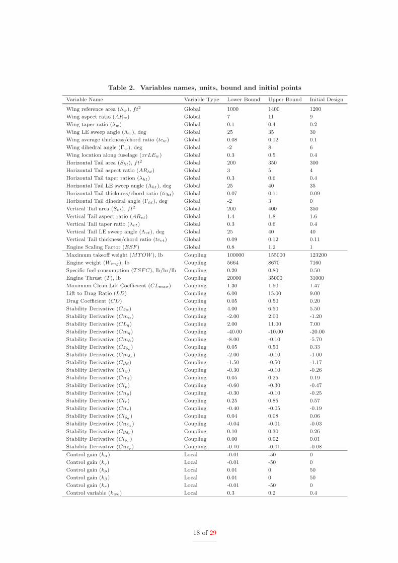
Table 2. Variables names, units, bound and initial points

Variable Name Variable Type Lower Bound Upper Bound Initial Design

Wing reference area (Sw), ft2 Global 1000 1400 1200

Wing aspect ratio (ARw) Global 7 11 9

Wing taper ratio (λw) Global 0.1 0.4 0.2

Wing LE sweep angle (Λw), deg Global 25 35 30

Wing average thickness/chord ratio (tcw) Global 0.08 0.12 0.1

Wing dihedral angle (Γw), deg Global -2 8 6

Wing location along fuselage (xrLEw) Global 0.3 0.5 0.4

Horizontal Tail area (Sht), ft2 Global 200 350 300

Horizontal Tail aspect ratio (ARht) Global 3 5 4

Horizontal Tail taper ration (λht) Global 0.3 0.6 0.4

Horizontal Tail LE sweep angle (Λht), deg Global 25 40 35

Horizontal Tail thickness/chord ratio (tcht) Global 0.07 0.11 0.09

Horizontal Tail dihedral angle (Γht), deg Global -2 3 0

Vertical Tail area (Svt), ft2 Global 200 400 350

Vertical Tail aspect ratio (ARvt) Global 1.4 1.8 1.6

Vertical Tail taper ratio (λvt) Global 0.3 0.6 0.4

Vertical Tail LE sweep angle (Λvt), deg Global 25 40 40

Vertical Tail thickness/chord ratio (tcvt) Global 0.09 0.12 0.11

Engine Scaling Factor (ESF ) Global 0.8 1.2 1

Maximum takeoff weight (MTOW ), lb Coupling 100000 155000 123200

Engine weight (Weng), lb Coupling 5664 8670 7160

Specific fuel consumption (TSFC), lb/hr/lb Coupling 0.20 0.80 0.50

Engine Thrust (T ), lb Coupling 20000 35000 31000

Maximum Clean Lift Coefficient (CLmax) Coupling 1.30 1.50 1.47

Lift to Drag Ratio (LD) Coupling 6.00 15.00 9.00

Drag Coefficient (CD) Coupling 0.05 0.50 0.20

Stability Derivative (Czα) Coupling 4.00 6.50 5.50

Stability Derivative (Cmα) Coupling -2.00 2.00 -1.20

Stability Derivative (CLq) Coupling 2.00 11.00 7.00

Stability Derivative (Cmq) Coupling -40.00 -10.00 -20.00

Stability Derivative (Cmα) Coupling -8.00 -0.10 -5.70

Stability Derivative (Czδe) Coupling 0.05 0.50 0.33

Stability Derivative (Cmδe) Coupling -2.00 -0.10 -1.00

Stability Derivative (Cyβ) Coupling -1.50 -0.50 -1.17

Stability Derivative (Clβ) Coupling -0.30 -0.10 -0.26

Stability Derivative (Cnβ) Coupling 0.05 0.25 0.19

Stability Derivative (Clp) Coupling -0.60 -0.30 -0.47

Stability Derivative (Cnp) Coupling -0.30 -0.10 -0.25

Stability Derivative (Clr) Coupling 0.25 0.85 0.57

Stability Derivative (Cnr) Coupling -0.40 -0.05 -0.19

Stability Derivative (Clδa) Coupling 0.04 0.08 0.06

Stability Derivative (Cnδa) Coupling -0.04 -0.01 -0.03

Stability Derivative (Cyδr) Coupling 0.10 0.30 0.26

Stability Derivative (Clδr) Coupling 0.00 0.02 0.01

Stability Derivative (Cnδr) Coupling -0.10 -0.01 -0.08

Control gain (kα) Local -0.01 -50 0

Control gain (kq) Local -0.01 -50 0

Control gain (kp) Local 0.01 0 50

Control gain (kβ) Local 0.01 0 50

Control gain (kr) Local -0.01 -50 0

Control variable (kwo) Local 0.3 0.2 0.4

18 of 29

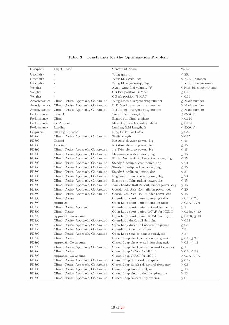
Table 3. Constraints for the Optimization Problem

Discipline Flight Phase Constraint Name Value

Geometry - Wing span, ft ≤ 260

Geometry - Wing LE sweep, deg ≤ H.T. LE sweep

Geometry - Wing LE edge sweep, deg ≤ V.T. LE edge sweep

Weights - Avail. wing fuel volume, ft3 ≤ Req. block fuel volume

Weights - CG fwd position % MAC ≥ 0.05

Weights - CG aft position % MAC ≤ 0.55

Aerodynamics Climb, Cruise, Approach, Go-Around Wing Mach divergent drag number ≥ Mach number

Aerodynamics Climb, Cruise, Approach, Go-Around H.T. Mach divergent drag number ≥ Mach number

Aerodynamics Climb, Cruise, Approach, Go-Around V.T. Mach divergent drag number ≥ Mach number

Performance Takeoff Takeoff field Length, ft ≤ 5500. ft

Performance Climb Engine-out climb gradient ≥ 0.024

Performance Go-Around Missed approach climb gradient ≥ 0.024

Performance Landing Landing field Length, ft ≤ 5000. ft

Propulsion All Flight phases Drag to Thrust Ratio ≤ 0.88

FD&C Climb, Cruise, Approach, Go-Around Static Margin ≥ 0.05

FD&C Takeoff Rotation elevator power, deg ≤ 15

FD&C Landing Rotation elevator power, deg ≤ 15

FD&C Climb, Cruise, Approach, Go-Around 1-g Trim elevator power, deg ≤ 15

FD&C Climb, Cruise, Approach, Go-Around Maneuver elevator power, deg ≤ 15

FD&C Climb, Cruise, Approach, Go-Around Pitch - Vel. Axis Roll elevator power, deg ≤ 15

FD&C Climb, Cruise, Approach, Go-Around Steady Sideslip aileron power, deg ≤ 20

FD&C Climb, Cruise, Approach, Go-Around Steady Sideslip rudder power, deg ≤ 15

FD&C Climb, Cruise, Approach, Go-Around Steady Sideslip roll angle, deg ≤ 5

FD&C Climb, Cruise, Approach, Go-Around Engine-out Trim aileron power, deg ≤ 20

FD&C Climb, Cruise, Approach, Go-Around Engine-out Trim rudder power, deg ≤ 15

FD&C Climb, Cruise, Approach, Go-Around Yaw - Loaded Roll Pullout, rudder power, deg ≤ 15

FD&C Climb, Cruise, Approach, Go-Around Coord. Vel. Axis Roll, aileron power, deg ≤ 20

FD&C Climb, Cruise, Approach, Go-Around Coord. Vel. Axis Roll, rudder power, deg ≤ 15

FD&C Climb, Cruise Open-Loop short period damping ratio ≥ 0.2, ≤ 2.0

FD&C Approach Open-Loop short period damping ratio ≥ 0.35, ≤ 2.0

FD&C Climb, Cruise, Approach Open-Loop short period natural frequency ≥ 1

FD&C Climb, Cruise Open-Loop short period GCAP for HQL I ≥ 0.038, ≤ 10

FD&C Approach, Go-Around Open-Loop short period GCAP for HQL I ≥ 0.096, ≤ 10

FD&C Climb, Cruise, Approach, Go-Around Open-Loop dutch roll damping ≥ 0.02

FD&C Climb, Cruise, Approach, Go-Around Open-Loop dutch roll natural frequency ≥ 0.5

FD&C Climb, Cruise, Approach, Go-Around Open-Loop time to roll, sec ≤ 3

FD&C Climb, Cruise, Approach, Go-Around Open-Loop time to double spiral, sec ≥ 8

FD&C Climb, Cruise Closed-Loop short period damping ratio ≥ 0.3, ≤ 2.0

FD&C Approach, Go-Around Closed-Loop short period damping ratio ≥ 0.5, ≤ 1.3

FD&C Climb, Cruise, Approach, Go-Around Closed-Loop short period natural frequency ≥ 1

FD&C Climb, Cruise Closed-Loop GCAP for HQL I ≥ 0.3, ≤ 3.3

FD&C Approach, Go-Around Closed-Loop GCAP for HQL I ≥ 0.16, ≤ 3.6

FD&C Climb, Cruise, Approach, Go-Around Closed-Loop dutch roll damping ≥ 0.08

FD&C Climb, Cruise, Approach, Go-Around Closed-Loop dutch roll natural frequency ≥ 0.5

FD&C Climb, Cruise, Approach, Go-Around Closed-Loop time to roll, sec ≤ 1.4

FD&C Climb, Cruise, Approach, Go-Around Closed-Loop time to double spiral, sec ≥ 12

FD&C Climb, Cruise, Approach, Go-Around Closed-Loop System Eigenvalues ≤ 0

19 of 29

Table 4. Control Effector Flapped Surface Characteristics

Control Effector/Parameters ηic ηoc cce/ccs max. Deflection, deg

Elevator 0.25 0.95 30% ±25

Ailerons 0.72 0.90 20% ±25

Rudder 0.10 1.00 26% ±15

Quadratic Programming (SQP) optimization algorithm30 is used at both the system and

the disciplinary levels. Proper scaling of the design variables, objectives and constraints is

enforced for the gradient-based optimizer to handle discrepancies along the feasible/near-

feasible descent direction when disciplinary constraints force incompatibilities among the

different subsystems. Objective function gradients are evaluated using finite differences.

Tolerances for the optimization procedure are defined on the order of 10−6 based on initial

studies to have a good compromise between the number of analysis calls at system and

subsystem levels and the optimal objective function. Convergence of the optimization pro-

cedure is reached when the search direction, maximum constraint violation and first-order

optimality measure are less than the specified tolerances.

V. Results

A. Optimized Designs and Comparisons

Table 5 shows selected variables and performance values for the multidisciplinary feasible

solution obtained from both the integrated and traditional design test cases. The geometric

configuration for both test cases is shown in Figure 9. While similar wing characteristics are

obtained for both designs, the horizontal and vertical tail geometry is significantly different

as seen in Figure 10. The concurrent consideration of flight dynamics and simultaneous

design of stability and control augmentation systems, leads to significant geometric changes

over the traditional design approach. The horizontal tail area is reduced to promote lower

static margins and improved aerodynamic efficiency. Similarly, the horizontal tail sweep in-

creases to avoid flow separation at high Mach numbers, hence it aggravates changes in wing

pitching moment. In addition, the increase in horizontal tail sweep delays the stall angle and

produces a more benign non-linear lift/stall behaviour. Furthermore, the wing apex location

is slightly moved forward along with a horizontal tail area reduction. This affects the center

of gravity of the aircraft and reduces its static margin. At the same time, the designed con-

trol system assures the required level of stability is achieved. The wing dihedral is increased

significantly to improve roll stability characteristics. In terms of performance, both test cases

meet the specified performance requirements. The reduction in exposed surface area for the

integrated aircraft design causes higher lift to drag values at all flight conditions, as shown

20 of 29

in Table 5. An air-range improvement of 510 nm is reached as compared to the traditional

design approach.

Table 5. Traditional and Integrated FD&C Optimization Results

Variable Name Traditional Integrated FD&C

Wing reference area (Sw), ft2 1400 1400

Wing aspect ratio (ARw) 11.00 11.00

Wing taper ratio (λw) 0.382 0.187

Wing LE sweep angle (Λw), deg 25.00 25.00

Wing average thickness/chord ratio (tcw) 0.117 0.105

Wing dihedral angle (Γw), deg 2.000 4.839

Wing location along fuselage (xrLEw) 0.39 0.35

Horizontal Tail area (Sht), ft2 328.43 250.35

Horizontal Tail aspect ratio (ARht) 4.88 3.07

Horizontal Tail taper ratio (λht) 0.561 0.525

Horizontal Tail LE sweep angle (Λht), deg 28.10 40.00

Horizontal Tail thickness/chord ratio (tcht) 0.088 0.073

Horizontal Tail dihedral angle (Γht), deg 0.00 -1.97

Vertical Tail area (Svt), ft2 250.04 250.01

Vertical Tail aspect ratio (ARvt) 1.8 1.4

Vertical Tail taper ration (λvt) 0.40 0.60

Vertical Tail LE sweep angle (Λvt), deg 31.17 40.00

Vertical Tail thickness/chord ratio (tcvt) 0.090 0.090

Engine Scaling Factor (ESF ) 0.8 0.8

Maximum takeoff weight (MTOW ), lb 120186 120413

Engine weight (Weng), lb 5664 5664

Specific fuel consumption (TSFC) @ Cruise, lb/hr/lb 0.5034 0.5034

Engine Thrust (T ) @ Takeoff, lb 25056 25056

Maximum Clean Lift Coefficient (CLmax) @ Cruise 1.483 1.501

Lift to Drag Ratio (LD) @ Cruise 17.050 17.653

Drag Coefficient (CD) @ Cruise 0.020 0.019

Lift to Drag Ratio (LD) @ Approach 9.681 10.311

Drag Coefficient (CD) @ Approach 0.183 0.143

Range, nm 5278.3 5788.7

Takeoff Field Length, ft 4284.1 4261.9

Landing Field Length, ft 3953.5 3945.2

Engine-out climb gradient 0.0681 0.0673

Missed approach climb gradient 0.0846 0.0906

Static Margin @ Cruise 0.3679 0.2424

Static Margin @ Approach 0.2528 0.1992

Table 6 shows a control power requirement comparison between the two design cases,

where bold values designate parameters which did not meet the required specifications (Ta-

ble 3). The integrated design shows reduced static margins due to the horizontal area

reduction. The design requires larger elevator deflection for takeoff rotation as compared to

the traditional aircraft, but it still within limits of the specified deflection constraint. Trim

requirements are similar for both designs. However, the integrated design requires less con-

trol power for trim at the approach condition, where the CG is critical at its maximum fwd

21 of 29

(a) Traditional Design (b) Integrated FD&C Design

Figure 9. Test Cases Optimal Configurations

0

20

40

60

80

100

−60 −40 −20 0 20 40 60Width [ft]

Aircraft Top View

Leng

th [f

t]

Traditional Design Range: 5278 nm MTOW: 120185 lb

Integrated FDC Design Range: 5788 nm MTOW: 120413 lb

Static Margins: − Cruise: 0.3679 − Approach: 0.2528

Static Margins: − Cruise: 0.2424 − Approach: 0.1992

(a) Top View

0 20 40 60 80 100

−10

0

10

20

30

Lenght [ft]

Aircraft Side View

Hei

ght [

ft]

0 20 40 60 80 100

−10

0

10

20

30

Lenght [ft]

Hei

ght [

ft]

Integrated FDC Design

Traditional Design

(b) Side View

Figure 10. Aircraft Configuration Comparison

22 of 29

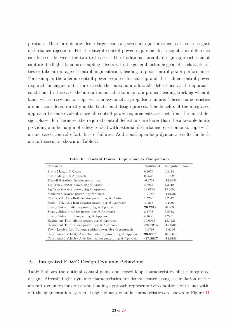
position. Therefore, it provides a larger control power margin for other tasks such as gust

disturbance rejection. For the lateral control power requirements, a significant difference

can be seen between the two test cases. The traditional aircraft design approach cannot

capture the flight dynamics coupling effects with the general airframe geometric characteris-

tics or take advantage of control-augmentation, leading to poor control power performance.

For example, the aileron control power required for sideslip and the rudder control power

required for engine-out trim exceeds the maximum allowable deflections at the approach

condition. In this case, the aircraft is not able to maintain proper heading tracking when it

lands with crosswinds or cope with an asymmetric propulsion failure. These characteristics

are not considered directly in the traditional design process. The benefits of the integrated

approach become evident since all control power requirements are met from the initial de-

sign phase. Furthermore, the required control deflections are lower than the allowable limits

providing ample margin of safety to deal with external disturbance rejection or to cope with

an increased control effort due to failures. Additional open-loop dynamic results for both

aircraft cases are shown in Table 7.

Table 6. Control Power Requirements Comparison

Parameter Traditional Integrated FD&C

Static Margin @ Cruise 0.3679 0.2424

Static Margin @ Approach 0.2528 0.1992

Takeoff Rotation elevator power, deg -6.2738 -14.0386

1-g Trim elevator power, deg @ Cruise 4.3247 4.3042

1-g Trim elevator power, deg @ Approach 19.6754 15.0588

Maneuver elevator power, deg @ Cruise -12.7531 -12.6707

Pitch - Vel. Axis Roll elevator power, deg @ Cruise 1.5796 2.7342

Pitch - Vel. Axis Roll elevator power, deg @ Approach 4.0268 6.4436

Steady Sideslip aileron power, deg @ Approach 26.7672 20.0638

Steady Sideslip rudder power, deg @ Approach 2.1798 6.5533

Steady Sideslip roll angle, deg @ Approach 4.1680 4.2251

Engine-out Trim aileron power, deg @ Approach 15.6064 18.5121

Engine-out Trim rudder power, deg @ Approach -28.1814 -15.0702

Yaw - Loaded Roll Pullout, rudder power, deg @ Approach -3.5798 -2.6306

Coordinated Velocity Axis Roll, aileron power, deg @ Approach 23.3895 16.5668

Coordinated Velocity Axis Roll rudder power, deg @ Approach -47.8037 -13.0146

B. Integrated FD&C Design Dynamic Behaviour

Table 8 shows the optimal control gains and closed-loop characteristics of the integrated

design. Aircraft flight dynamic characteristics are demonstrated using a simulation of the

aircraft dynamics for cruise and landing approach representative conditions with and with-

out the augmentation system. Longitudinal dynamic characteristics are shown in Figure 11

23 of 29

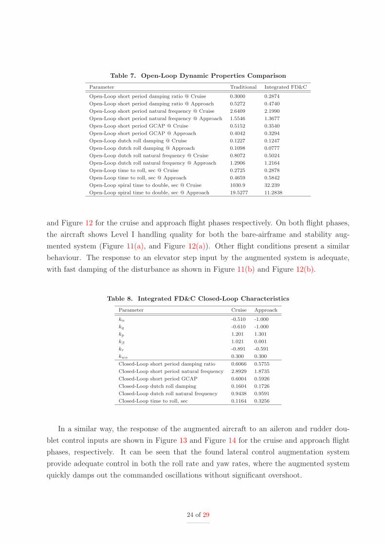
Table 7. Open-Loop Dynamic Properties Comparison

Parameter Traditional Integrated FD&C

Open-Loop short period damping ratio @ Cruise 0.3000 0.2874

Open-Loop short period damping ratio @ Approach 0.5272 0.4740

Open-Loop short period natural frequency @ Cruise 2.6409 2.1990

Open-Loop short period natural frequency @ Approach 1.5546 1.3677

Open-Loop short period GCAP @ Cruise 0.5152 0.3540

Open-Loop short period GCAP @ Approach 0.4042 0.3294

Open-Loop dutch roll damping @ Cruise 0.1227 0.1247

Open-Loop dutch roll damping @ Approach 0.1098 0.0777

Open-Loop dutch roll natural frequency @ Cruise 0.8072 0.5024

Open-Loop dutch roll natural frequency @ Approach 1.2906 1.2164

Open-Loop time to roll, sec @ Cruise 0.2725 0.2878

Open-Loop time to roll, sec @ Approach 0.4659 0.5842

Open-Loop spiral time to double, sec @ Cruise 1030.9 32.239

Open-Loop spiral time to double, sec @ Approach 19.5277 11.2838

and Figure 12 for the cruise and approach flight phases respectively. On both flight phases,

the aircraft shows Level I handling quality for both the bare-airframe and stability aug-

mented system (Figure 11(a), and Figure 12(a)). Other flight conditions present a similar

behaviour. The response to an elevator step input by the augmented system is adequate,

with fast damping of the disturbance as shown in Figure 11(b) and Figure 12(b).

Table 8. Integrated FD&C Closed-Loop Characteristics

Parameter Cruise Approach

kα -0.510 -1.000

kq -0.610 -1.000

kp 1.201 1.301

kβ 1.021 0.001

kr -0.891 -0.591

kwo 0.300 0.300

Closed-Loop short period damping ratio 0.6066 0.5755

Closed-Loop short period natural frequency 2.8929 1.8735

Closed-Loop short period GCAP 0.6004 0.5926

Closed-Loop dutch roll damping 0.1604 0.1726

Closed-Loop dutch roll natural frequency 0.9438 0.9591

Closed-Loop time to roll, sec 0.1164 0.3256

In a similar way, the response of the augmented aircraft to an aileron and rudder dou-

blet control inputs are shown in Figure 13 and Figure 14 for the cruise and approach flight

phases, respectively. It can be seen that the found lateral control augmentation system

provide adequate control in both the roll rate and yaw rates, where the augmented system

quickly damps out the commanded oscillations without significant overshoot.

24 of 29

10−1

100

10−2

10−1

100

101

Damping Ratio, Zsp

CA

P, (

g−1 )(

sec−

2 )

SHORT PERIOD DYNAMIC REQUIREMENTS Cruise Flight Phase

LEVEL 1

LEVEL 2

o − Unaugmented Aircraftx − Augmented Aircraft

(a) Short-Period Handling Qualities

0 0.5 1 1.5 2 2.5 3 3.5−0.5

−0.45

−0.4

−0.35

−0.3

−0.25

−0.2

−0.15

−0.1

−0.05

0

Time [sec]

α/δe

q/δe

(b) Closed-Loop Response to Control Step

Figure 11. Cruise Longitudinal Dynamics Characteristics

10−1

100

10−2

10−1

100

101

Damping Ratio, Zsp

CA

P, (

g−1 )(

sec−

2 )

SHORT PERIOD DYNAMIC REQUIREMENTS Landing Approach Flight Phase

LEVEL 1

LEVEL 2

LEVEL

3

o − Unaugmented Aircraftx − Augmented Aircraft

(a) Short-Period Handling Qualities

0 1 2 3 4 5 6 7 8 9−0.7

−0.6

−0.5

−0.4

−0.3

−0.2

−0.1

0

Time [sec]

α/δe

q/δe

(b) Closed-Loop Response to Control Step

Figure 12. Landing Approach Longitudinal Dynamics Characteristics

25 of 29

0 5 10 15 20 25 30−10

−5

0

5

10

Time [sec]

Roll Rate Response to Aileron Control Doublet

0 5 10 15 20 25 30−10

−5

0

5

10

Time [sec]

Sideslip Angle and Yaw Rate Response to Rudder Control Doublet

p [deg/sec]Control Doublet [deg]

β [deg]r [deg/sec]Control Doublet [deg]

Figure 13. Cruise Closed-Loop Lateral Dynamics Response to Controls Doublet

0 5 10 15 20 25 30−6

−4

−2

0

2

4

6

Time [sec]

Roll Rate Response to Aileron Control Doublet

0 5 10 15 20 25 30−6

−4

−2

0

2

4

6

Time [sec]

Sideslip Angle and Yaw Rate Response to Rudder Control Doublet

p [deg/sec]Control Doublet [deg]

β [deg]r [deg/sec]Control Doublet

Figure 14. Landing Approach Closed-Loop Lateral Dynamics Response to Controls Doublet

26 of 29

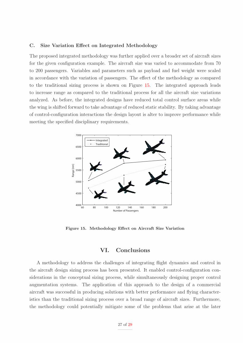
C. Size Variation Effect on Integrated Methodology

The proposed integrated methodology was further applied over a broader set of aircraft sizes

for the given configuration example. The aircraft size was varied to accommodate from 70

to 200 passengers. Variables and parameters such as payload and fuel weight were scaled

in accordance with the variation of passengers. The effect of the methodology as compared

to the traditional sizing process is shown on Figure 15. The integrated approach leads

to increase range as compared to the traditional process for all the aircraft size variations

analyzed. As before, the integrated designs have reduced total control surface areas while

the wing is shifted forward to take advantage of reduced static stability. By taking advantage

of control-configuration interactions the design layout is alter to improve performance while

meeting the specified disciplinary requirements.

60 80 100 120 140 160 180 2004000

4500

5000

5500

6000

6500

7000

Number of Passengers

Ra

ng

e [

nm

]

Integrated

Traditional

Figure 15. Methodology Effect on Aircraft Size Variation

VI. Conclusions

A methodology to address the challenges of integrating flight dynamics and control in

the aircraft design sizing process has been presented. It enabled control-configuration con-

siderations in the conceptual sizing process, while simultaneously designing proper control

augmentation systems. The application of this approach to the design of a commercial

aircraft was successful in producing solutions with better performance and flying character-

istics than the traditional sizing process over a broad range of aircraft sizes. Furthermore,

the methodology could potentially mitigate some of the problems that arise at the later

27 of 29

stages of the design process as compliance with the most general flight dynamic certification

requirements is assured from the conceptual stage, reducing time and cost in the engineering

development cycle.

References

1Kehrer, W., “Design Evolution of the Boeing 2707-300 Supersonic Transport,” 43rd AGARD Flight

Mechanics Panel Meeting, Aircraft Design Integration and Optimization, No. AGARD CP-147, October

1973.

2Current State of the Art On Multidisciplinary Design Optimization (MDO), General Publication Series,

American Institute of Aeronautics and Astronautics, Washington, DC, January 1991.

3Birkenstock, W., “Unstable Aircraft Design: The Computer at the Controls,” Flug Revue, Vol. 9,

September 1999, pp. 74.

4Dermis, T., Nalepka, J., Thompson, D., and Dawson, D., “Fly-by-Light: The Future of Flight Control

Technology,” Technology Horizons Magazine, Air Force Research Laboratory Air Vehicles Directorate, , No.

Report VA-04-12, April 2005.

5Nicolai, L., Fundamentals of Aircraft Design, METS Inc., San Jose, CA, 2nd ed., 1984.

6Raymer, D., Aircraft Design: A Conceptual Approach, AIAA Education Series, American Institute of

Aeronautics and Astronautics, Washington, DC, 3rd ed., 1999.

7Jenkinson, L., Simpkin, P., and Rhodes, D., Civil Jet Aircraft Design, Arnold, London, UK, 1st ed.,

1999.

8Kay, J., Mason, W., Lutze, F., and Durham, W., “Control Authority Issues in Aircraft Conceptual

Design: Critical Conditions, Estimation Methodology, Spreadsheet Assessment, Trim and Bibliography,”

Tech. Rep. VPI-Aero-200, Virginia Polytechnic Institute and State University, Department of Aerospace

and Ocean Engineering, Blacksburg, VA, November 1993.

9Chudoba, B., Stability and Control of Conventional and Unconventional Aircraft Configurations - A

Generic Approach, Books on Demand GmbH, Norderstedt, Germany, 1st ed., January 2002.

10Sahasrabudhe, V., Celi, R., and Tits, A., “Integrated Rotor-Flight Control System Optimization

with Aeroelastic and Handling Qualities Constraints,” AIAA Journal of Guidance, Control and Dynamics,

Vol. 20, No. 2, March-April 1997, pp. 217–224.

11Holloway, R. and Burris, P., “Aircraft Performance Benefits from Modern Control Systems Technol-

ogy,” AIAA Journal of Aircraft , Vol. 7, No. 6, Nov-Dec 1970, pp. 550–553.

12Sobieszczanski-Sobieski, J., “Multidisciplinary Design Optimization: An Emerging New Engineering

Discipline,” World Congress of Optimal of Structural Systems, Rio de Janeiro, Brazil, August 1993.

13Braun, R., Gage, P., Kroo, I., and J., S.-S., “Implementation and Performance Issues in Collaborative

Optimization,” 5th AIAA/USAF Symposium on Multidisciplinary Analysis and Optimization, No. Paper

1996-4017, AIAA, Bellevue, WA, September 4-6 1996.

14Chudoba, B., “Stability and Control Aircraft Design and Test Condition Matrix,” Tech. Rep. Technical

Report EF-039/96, Daimler-Benz Aerospace Airbus, Hamburg, Germany, September 1996.

15Chudoba, B. and Cook, M., “Identification of Design-Constraining Flight Conditions for Conceptual

Sizing of Aircraft Control Effectors,” AIAA Atmospheric Flight Mechanics Conference and Exhibit , No.

Paper 2003-5386, Austin, TX, August 11-14 2003.

28 of 29

16Steer, A., “Design Criteria For Conceptual Sizing of Primary Flight Controls,” The Aeronautical

Journal , Vol. 108, No. 1090, December 2004, pp. 629–641.

17“U.S. Military Handbook MIL-HDBK-1797,” Tech. rep., Department of Defense, Washington, DC,

December 1997.

18Etkin, B. and Reid, L., Dynamics of Flight, Stability and Control , John Wiley & Sons, New York, NY,

3rd ed., 1996.

19Anon, “MIL SPEC - Flying Qualities of Piloted Airplanes,” Tech. Rep. MIL-F-8785C, U.S. Government

Printing Office, Washington, DC, November 1980.

20Bihrle, Jr., W., “A Handling Qualities Theory for Precise Flight Path Control,” Tech. Rep. Technical

report AFFDL-TR-65-198, Air Force Flight Dynamics Lab., Wright-Patterson AFB, OH, June 1966.

21Gautrey, J. and Cook, M., “A Generic Control Anticipation Parameter for Aircraft Handling Qualities

Evaluation,” The Aeronautical Journal , Vol. 102, No. 1013, March 1998, pp. 151–159.

22Anderson, M. and Mason, W., “An MDO Approach to Control-Configured-Vehicle Design,” 6Th

AIAA/NASA/ISSMO Symposium on Multidisciplinary Analysis and Optimization, No. Paper 1996-4058,

Bellevue, WA, September 4-6 1996.

23Torenbeek, E., Synthesis of Subsonic Airplane Design, Delft University Press and Kluwer Academic

Publishers, Delft, The Netherlands, sixth ed., 1990.

24Chai, S., Crisafuli, P., and Mason, W., “Aircraft Center of Gravity Estimation in Conceptual Design,”

1st AIAA Aircraft Engineering, Technology, and Operations Congress, No. Paper 95-3882, Los Angeles, CA,

September 19-21 1995.

25Roskam, J., Airplane Design, Vol. 1-8, DARcorporation, Ottawa, KS, 1st ed., 1998.

26Malone, B. and Mason, W., “Multidisciplinary Optimization in Aircraft Design Using Analytic Tech-

nology Models,” AIAA Journal of Aircraft , Vol. 32, No. 2, March-April 1995, pp. 431–438.

27Fink, R., “USAF Stability and Control DATCOM,” Tech. rep., Air Force Flight Dynamics Lab.,

Wright-Patterson AFB, OH, 1975.

28Unit, E. E. S. D., “Introduction to Aerodynamic Derivatives Equations of Motion and Stability,” Tech.

Rep. Item No. 86021, ESDU International plc, London, UK, 1987.

29Schmidt, L., Introduction to Aircraft Flight Dynamics, AIAA Education Series, American Institute of

Aeronautics and Astronautics, Reston, VA, 1st ed., 1998.

30Nocedal, J. and Wright, S., Numerical Optimization, Series in Operational Research, Springer-Verlag,

New York, NY, 1st ed., 1999.

29 of 29

Documents

A Multidisciplinary Optimization Framework for Control