Mishra et al. 1

A Multi-Objective Optimization Model for Transit Fleet Resource 1

Allocation 2

3 4

By 5 6

Sabyasachee Mishra, Ph.D., P.E. 7 Assistant Professor 8

Department of Civil Engineering 9 University of Memphis 10 Memphis, TN 38152 11 P:+1-901-678-2000 12

Email: smishra@memphis.edu 13 14

Sushant Sharma, Ph.D. 15 Research Associate 16

NEXTRANS Center, Regional University Transportation Center 17 Purdue University, West Lafayette 18

P: +1-765-496-9768 19 Email: sharma57@purdue.edu 20

21 22

Tom V Mathew, Ph.D. 23 Professor 24

Department of Civil Engineering, 25 Indian Institute of Technology Bombay, 26

Powai, Mumbai - 400076, India. 27 P: +91-22-2576 7349 28

Email: tvm@civil.iitb.ac.in 29 30

Snehamay Khasnabis, Ph.D., P.E. 31 Professor Emeritus 32

Department of Civil and Environmental Engineering 33 Wayne State University 34

Detroit, MI 48202 35 Phone: +1-313- 577-3915 36 Email: skhas@wayne.edu 37

38 39 40

Word Count: 41 Number of Tables: 42 Number of Figures: 43

Total Count: = 5,128 + (9 x250) = 7,378 44 Date Submitted: November 2012 45

46 47 48

Submitted for Publication and Peer Review and for Compendium of Papers CD-ROM at the Annual 49 Meeting of the Transportation Research Board (TRB) in January 2013 50

Mishra et al. 2

Abstract 1

State and local transit agencies require government support to preserve their aging transit fleet. With 2 passage of time, transit fleet gets older and requires maintenance cost to keep it operational. To provide 3 services at a desired level, transit agencies require maintaining a minimum fleet size. Two imperative 4 considerations from transit planning viewpoint are (1) remaining life of the total fleet, and (2) cost 5 required to maintain the fleet size. When the former is a quality measure indicating the health of the fleet, 6 the latter is an economic measure requiring minimum expenditure levels. Ideally, the agencies would like 7 to maximize the total remaining life of the fleet and minimize the total cost required to maintain the fleet 8 size. In this paper, the authors propose a multi-objective optimization model (MO) to simultaneously 9 incorporate both objectives when subjected to budget and a number of operational constraints. The MO 10 problem is solved by using classical weight sum approach by employing Branch and Bound Algorithm 11 (BBA) that has proven to be better than other solution methodologies. The MO resulted in pareto optimal 12 solutions with the possible trade-off between the two objectives. The model is applied to a real large scale 13 transit fleet system in the state of Michigan, U.S. The case study results demonstrate, the proposed model 14 is compact, efficient, robust and suitable for long range planning with multiple solutions to choose from a 15 pareto optimal frontier. The correlation between decision variables and objective functions has been 16 investigated in-depth and provides important insights. The proposed model can act as a tool for resource 17 allocation for transit fleet among agencies for state and local agencies. 18

Keywords: transit fleet, multi-objective optimization, branch and bound algorithm, pareto optimal 19

1. Introduction 20

A number of state Departments of Transportation (DOT) and their local transit agencies are concerned 21 about the escalating costs of new buses and lack of funds to keep up with their replacement needs. The 22 cost of replacing the aging transit fleet in the US to maintain current performance levels is estimated to 23 exceed one billion dollars annually (1, 2). The addition of new buses to the existing fleet of any transit 24 agency is a capital intensive process. In the US, the federal government provides a bulk of the capital 25 funds needed to replace the aging transit fleet, with the requirement of a minimum matching support 26 (usually 20%) from non-federal sources. 27

A bus that completes its service life should ideally be replaced. However, lack of capital funds 28 often prevents state DOTs from procuring new buses for their constituent agencies. Several rebuilding 29 alternatives to bus replacement are available to the transit industry that can be classified under two 30 generic categories: bus rehabilitation and bus remanufacturing. A number of studies conducted between 31 1980 and 2000 explored the economics of replacement of buses versus rebuilding of existing buses. Most 32 of these studies found that up to certain limits, it is cost-effective to rebuild an existing bus thereby 33 extending the life by a few years with a fraction of the procurement cost of a new bus. The problem 34 addressed is typical to a state DOT in the US that supports the fleet management of its constituent transit 35 agencies. While replacing the aging fleet is the most desirable option from a quality point of view, 36 budgetary constraints require transit agencies to use a combination of new and old buses to provide 37 services for their customers. Thus the challenge before the agency lies in finding an optimum combination 38 of new and old buses by partially replacing and partially preserving the existing fleet. Two imperative and 39 conflicting measures in the resource allocation are (1) fleet quality measure; and (2) economic measure. 40 These two measures are quantified in the following section. 41

Fleet Quality Measure 42

A quality measure can be considered as the remaining life of the fleet system. An agency’s objective is to 43 maximize the quality measure. Recent studies attempted to improve upon the original model by 44 suggesting both structural and methodological changes (3, 4). These studies attempted to maximize the 45

Mishra et al. 3

quality of the bus fleet by optimizing different surrogates of Remaining Life (RL)1. In this context, Total 1 Weighted Average Remaining Life (TWARL) for one agency can be defined as: 2

𝑇𝑊𝐴𝑅𝐿 = ∑∑ 𝑓𝑖𝑗

𝑚𝑟𝑖𝑗𝑚

𝑗

∑ 𝑓𝑖𝑗𝑚

𝑗𝑖

(1)

where, 𝑓𝑖𝑗𝑚 is the number of buses for an agency i with remaining life of j years on mth planning year; 3

𝑟𝑖𝑗𝑚 is the remaining life of j years for an agency i on mth planning year for a corresponding bus; i is the 4

agency, j is the remaining life, and m is the planning year in consideration. Mathew et al. (2010) 5 reformulated the existing model (3) by maximizing Total System Weighted Average Remaining Life 6 (TSWARL) defined as the sum of TWARL over the planning period in consideration (4), i.e. ∑ 𝑇𝑊𝐴𝑅𝐿𝑚 , 7 where: 8

𝑇𝑆𝑊𝐴𝑅𝐿 = ∑ ∑∑ 𝑓𝑖𝑗

𝑚𝑟𝑖𝑗𝑚

𝑗

∑ 𝑓𝑖𝑗𝑚

𝑗𝑖𝑚

(2)

Both TWARL and TSWARL can be looked upon as surrogates of the quality of the fleet and 9 need to be maximized. In the remainder of this paper, we will be using abbreviations of these quality 10 measures. Further, research presented in this paper is also based upon an alternative approach of cost 11 minimization as another economic measure. 12

Economic Measure 13

In terms of economic measure the agency has scarcity in funding to manage the fleet so that the fleet size 14 is maintained with minimum cost. Net Present Cost (NPC) is used in a number of studies to measure the 15 expenditure. For the proposed resource allocation problem, NPC is defined as the sum of spending in 16 improvement of transit options when the dollar value of the expenditure is brought to its present value 17 using appropriate interest rate throughout the planning period. If 𝑥𝑖,𝑘

𝑚 is the number of buses chosen for 18

agency i, for improvement option k, and for time period m; 𝑐𝑘𝑚 is the cost of improvement option k in year 19

m; and ∅ is the interest rate/discount factor then NPC can be measured as 20

𝑁𝑃𝐶 = ∑ ∑ ∑𝑥𝑖,𝑘

𝑚 ∗ 𝑐𝑘𝑚

(1 + ∅)𝑚

𝑘𝑖𝑚

(3)

21

The agency’s objective is to minimize the NPC while maintaining the quality measure to minimum 22 standards. 23

Measure Preference 24

If the agency’s objective is to maximize the quality measure, that maximum value may not be attainable 25 within a given budget constraint. Both of the above mentioned measures are conflicting, and an agency 26 would like to invest minimum amount (in terms of net present cost) over planning period to obtain the 27 best fleet quality measure possible. In a true sense both objectives (to maximize fleet quality and to 28 minimize the NPC) should be considered simultaneously. In this paper, we present a multi-objective 29 optimization (MO) framework rather minimizing or maximizing each objective separately. MO results in 30 a set of pareto optimal solutions as opposed to just one solution, and it allows the agency to investigate a 31

1RL can be defined as the difference between the minimum normal service life (MNSL) and the age of the bus. The

MNSL of a medium-sized bus, the subject matter of this study is taken as seven years per guidelines of the U. S.

Department of Transportation.

Mishra et al. 4

trade-off between the two objectives. Pareto-optimal solutions are those in which it is impossible to make 1 one objective better off without necessarily making the other objective(s) worse off (5). The remainder of 2 the paper is organized as follows. A literature review is presented in the next section along with the need 3 of the research followed by methodology. The case study section shows the structure of a real world data. 4 Results and discussion section includes the findings of the research. Lastly, the summary of research and 5 future steps are presented in the conclusion section. 6

2. Literature Review 7

Literature review section is organized into three areas: (1) transit fleet improvement options, (2) 8 quantitative measures for fleet management, (3) multi-objective optimization applications for transit. The 9 review is not intended to be exhaustive, but to highlight some of the general trends in addressing the 10 allocation problem. 11

Transit Fleet Improvement Options 12

Transit improvement options drew significant attention in the 1980s, and received renewed research 13 interest in the late 1990s. A number of studies found replacement, rehabilitation, and remanufacturing are 14 the preferred options (6-9). The literature review clearly showed that remanufacturing and rehabilitation 15 of buses, if done properly, can be a cost-effective option. The studies mentioned above stressed the 16 importance of proper preventive maintenance as a primary factor contributing to the success of 17 rehabilitation programs. These studies emphasized that rehabilitation, “if properly done,” can be a 18 successful strategy, clearly referring to the quality of maintenance and steps taken by the agency to 19 prevent major breakdowns in machine components or bus body infrastructure. For the purpose of this 20 paper, the following terms are adapted from the literature. 21

i. Replacement (REPLACE): Process of retiring an existing vehicle and procuring a completely 22 new vehicle. Vehicles replaced using federal dollars must have completed their MNSL 23 requirements. 24

ii. Rehabilitation (REHAB): Process by which an existing vehicle is rebuilt to the original 25 manufacturer’s specification, with primary focus on the vehicle interior and mechanical system. 26

iii. Remanufacturing (REMANF): Process by which the structural integrity of the vehicle is restored 27 to original design standards. This includes remanufacturing the body, the chassis, the drive train, 28 and the vehicle interior and mechanical system. 29

Note: The generic term ‘REBUILD’ has been used in this paper to mean Rehabilitation and or 30 Remanufacturing. 31

Quantitative Measures for Fleet Management 32

Service life maximization is the most commonly adopted measure of effectiveness (MOE) for the 33 resource allocation in conjunction with budgetary constraints. Some prominent bus maintenance 34 management studies include: bus maintenance programs for cost-effective reliable transit service (10-11), 35 a generalized framework for transit bus maintenance operation (12), manpower allocation for transit bus 36 maintenance program (13), framework for evaluating a transit agency's maintenance program (14), a 37 simulation model for comparing a bus maintenance system's performance under various repair policies 38 (15), and performance indicators for maintenance management (16). These problems primarily cater to an 39 operator, who is concerned with the day to day maintenance for an efficient fleet operation. 40

Another commonly adopted MOE for transit resource allocation is in terms of monetary units. 41 The performance measures frequently used in literature are maximization of revenue, return, or profits, 42

Mishra et al. 5

benefit to cost ratio, internal rate of return, pay off period, cost effectiveness (17-23). NPC is a widely 1 understood and used MOE in transportation decision making. Minimization of NPC has been used as a 2 MOE for evaluation of transit level of service (24); for evaluation of rail transit investment priorities (25); 3 for finding the optimal bus transit service coverage in an urban corridor (26); for modeling the timing of 4 public infrastructure projects (27); for a decision support tool for evaluating investments in transit 5 systems fare collection(28); for analyzing induced demand with introduction of new transit system (29); 6 for analyzing transportation impacts on economic development (30); for analyzing externalities associated 7 with light rail investment (31); for resource allocation among transit agencies(3-4); and for project 8 selection problem under uncertainty (32). 9

Multi-Objective Optimization in Transit Application 10

Research on multi-objective optimization application for transit has been limited in the literature. Lianbo 11 et al. (33) studied the train planner for urban rail transit; they proposed a multi-objective optimization 12 model for train formation, train counts as well as operation periods considering factors such as transport 13 capacity, the requirements of traffic organization, corporation benefits, passenger demands, and passenger 14 choice behavior under multi-train-routing mode. Desai et al. (34) studied the fleet management for 15 electric vehicles by minimizing fuel economy and pollutants (HC; CO; NOx); Mauttone and Urquhart 16 (35) analyzed a MO transit network design problem and obtained non-dominated solutions representing 17 different trade-off levels between the conflicting objectives of users and operators. Wu et al. (36) used 18 MO to obtain optimal transit stops under American Disabilities Act (ADA). Among the solution 19 methodologies, Genetic Algorithm (GA) is extensively used to model multi-objective problems. 20 However, in this study we will be using branch and bound analysis (BBA) and not genetic algorithm 21 (GA), as Mathew et. al. (2010) reports that GA provides inferior solution compared to BBA in solving 22 transit resource allocation problems (4). 23

3. Motivation 24

While some studies described in literature made a contribution towards formulating and solving the transit 25 resource/fleet allocation problem and others applied MO in transit, to the best of authors knowledge the 26 above mentioned objectives of transit fleet resource allocation have never been investigated 27 simultaneously. Most of the similar studies in literature have following limitations: 28

In literature only fleet quality measure (TWARL or TSWARL) has been maximized without 29 considering any economic measure (like Net Present Cost (NPC)) other than available budget. 30

A key gap in literature has been in terms of inability to control NPC. The previous studies have 31 only considered NPC as a byproduct of the process of maximizing TSWARL. In practice, while 32 considering the investment for fleet improvement, state DOTs are concerned about economic 33 measures such as NPC for spending in a multi-year planning period, that may become a critical 34 factor in the final decision making process. Thus, minimizing NPC rather obtaining it as a 35 byproduct would have more significant implication to the transit agency. 36

In literature there is a lack of understanding of relationship between both performance measures 37 TSWARL and NPC. Further, the possible relationship between different improvement options 38 such as REHAB, REMANF, and REPLACE and both measures (TSWARL and NPC) has not 39 been studied explicitly. This paper investigates the correlation between each option and 40 performance measures. Moreover, in this paper we also show that in a multi-year planning period 41 how TWARL of a single year is related to either and both performance measures. 42

43

Mishra et al. 6

1

4. Methodology 2 3 As mentioned earlier, in this study we formulate a multi-objective optimization problem with the first 4 objective of minimization of NPC of the total investment of the fleet for all the agencies over the entire 5 planning period and the second objective of maximization of TSWARL, subjected to budget, demand, 6 rebuild, and non-negativity constraints. For ease in understanding the complete formulation there is a 7 simple explanation provided in front of each equation. The formulation notations are given below 8 followed by the formulation and their explanation: 9

Variables Explanation

𝑏𝑚 : budget available for mth planning year

𝑐𝑘𝑚 : cost of implementation of the improvement program k on mth year

𝑓𝑖,𝑗𝑚 : Number of buses for an agency i with remaining life of j years on mth planning year

𝑙𝑘 : additional year added to the life of the bus due to improvement program k, 𝑙𝑘 ∈ {2,3,4,7}

𝑟𝑖𝑗𝑚 : number of existing buses with remaining life of j years for an agency i on mth planning year

𝑥𝑖𝑗𝑚 : number of buses which received remaining life of j years for an agency i on mth planning year

due to the improvement program

𝑦𝑖𝑘𝑚 : number of buses chosen for the improvement program k adopted for an agency i on mth

planning year

𝛿𝑖,(𝛼,𝛽)𝑚 : number of buses already improved by , years due to rehabilitation in the mth planning year

for agency i, (𝛼, 𝛽 ∈ {2,3})

𝛿𝑖,(𝛾)𝑚 : number of buses already improved by years due to remanufacture in the mth planning year for

agency i, (𝛾 ∈ {4})

∅ The interest rate used for NPC

A : total number of agencies

B : total budget available for the project for all planning years

i : 1, 2, …,A, the subscript for a transit agency

j : 1, 2, …,Y, the subscript for remaining life

k : 1,2,…., P the subscript used for improvement program

m : 1, 2, …,N, the subscript used planning year

N : number of years in the planning period

P : number of improvement programs

REHAB1 : the first improvement program- rehabilitation of bus yielding (=2) additional years

REHAB2 : the second improvement program- rehabilitation of bus yielding (=3) additional years

REMANF : the third improvement program- rehabilitation of bus yielding (=4)additional years

REPLACE : the last improvement program-replacement of bus yielding 7 additional years

TSWARL : Total System Weighted Average Remaining Life , 𝑇𝑆𝑊𝐴𝑅𝐿 = ∑ 𝑇𝑊𝐴𝑅𝐿𝑚

TWARL : Total Weighted Average Remaining Life=𝑇𝑊𝐴𝑅𝐿 = ∑ 𝑊𝐴𝑅𝐿𝑖𝑖

WARLi : Weighted Average Remaining Life for agency i=𝑊𝐴𝑅𝐿𝑖 =

∑ 𝑓𝑖𝑗𝑚𝑟𝑖𝑗

𝑚𝑗

∑ 𝑓𝑖𝑗𝑚

𝑗

Y : minimum service life of buses

Zx : The objective function as minimization of NPV for the resource allocation in the planning

period

ρ : Weight factor 0 ≤ ρ ≤ 1

Mishra et al. 7

Mathematical Construct Explanation Eq.#

Minimize Z = (1- ρ) *�̅�𝑥1 – ρ *�̅�𝑥

2; ∀ 0 ≤ ρ ≤ 1

Overall Objective: weighted sum of normalized

net present cost (NPC) and sum of normalized

total system weighted average remaining life of

the fleet (TSWARL). As we are minimizing

NPC and maximizing TSWARL, the value of

the objective function TSWARL is to be

negative to represent the overall problem as

minimization problem. The weight (ρ)

considered here is between 0 and 1.

(4)

𝑍𝑥1 = ∑ ∑ ∑

𝑥𝑖,𝑘𝑚 ∗ 𝑐𝑘

𝑚

(1 + ∅)𝑚

𝑃

𝑘=1

𝐴

𝑖=1

𝑁

𝑚=1

Objective function 1 : net present cost of the

transit fleet resource allocation (NPC)

(5)

𝑍𝑥2 = ∑ ∑

∑ (𝑟𝑖,𝑗𝑚 + 𝑥𝑖,𝑗

𝑚) ∗ 𝑗𝐽𝑗=1

∑ (𝑟𝑖,𝑗𝑚 + 𝑥𝑖,𝑗

𝑚 )𝐽𝑗=1

𝐴

𝑖=1

𝑁

𝑚=1

Objective function 2 : sum total of the weighted

average remaining life of the fleet of all the

constituent agencies for the whole planning

period (TSWARL)

(6)

Subjected to following constraints

∑ ∑ ∑ 𝑦𝑖𝑘𝑚 ∗ 𝑐𝑘

𝑚 <

𝑃

𝑘=1

𝐴

𝑖=1

𝑁

𝑚=1

∑ 𝑏𝑚

𝑁

𝑚=1

, ∀𝑚

Constraint: Total cost of improving the buses

for different improving schemes, agencies and

over a planning period should not exceed

budget for the planning period

(7)

∑ 𝑏𝑚

𝑁

𝑚=1

= 𝐵

Constraint: Planning period budget is equal to

the sum available budget for each year, where

budget is a priori.

(8)

∑ 𝑦𝑖𝑘𝑚

𝑃

𝑘=1

= 𝑟𝑖𝑗𝑚 , ∀𝑖, 𝑚, 𝑗

Constraint: The buses that are improved under

improvement scheme k are the ones that have

completed their minimum normal service life

and have remaining life j

(9)

𝑦𝑖𝛾𝑚 = ∑ 𝛿𝑖,(𝛼𝛽)

𝑚

𝛼𝛽

+ 𝛿𝑖,(𝛾)𝑚 ∀𝑖, 𝑚, 𝑗

Constraint: All the buses that have completed

their minimum normal service life (10)

𝑦𝑖𝛾𝑚 = ∑ 𝛿𝑖,(𝛼𝛽)

𝑚

𝛼𝛽

+ 𝛿𝑖,(𝛾)𝑚 ∀𝑖, 𝑚, 𝑗

∀𝛼, 𝛽 ∈ {2,3}, 𝛾{4}

Constraint: The buses that have been

rehabilitated twice or remanufactured once will

be replaced

(11)

𝑦𝑖𝛾𝑚 > 0 Constraint: Non-negativity constraint. Number

of buses chosen for improvement should be

greater than 0

(12)

𝑥𝑖𝑗𝑚 = {

𝑦𝑖𝑘𝑚, 𝑖𝑓𝑗 = 𝑙𝑘 , 𝑙𝑘 ∈ {2,3,4,7}

0 , 𝑂𝑡ℎ𝑒𝑟𝑤𝑖𝑠𝑒

Constraint: The life of the buses is improved by

either two, three, or four years for a re-built bus

and by seven years for a new bus

(13)

𝛿𝑖,(𝛼𝛽)𝑚 = {

𝑚𝑖𝑛 {𝑦𝑖𝛼𝑚−(𝛼+𝛽)

, 𝑦𝑖𝛽𝑚−𝛼} 𝑖𝑓𝑚 ≥ 𝛼 + 𝛽, ∀𝑚 > 𝛼 + 𝛽,

0 , 𝑂𝑡ℎ𝑒𝑟𝑤𝑖𝑠𝑒

Constraint: Auxiliary

constraint of Eq. (7),

represents replacement

option after 𝛼 + 𝛽 years

(REHAB)

(14)

Mishra et al. 8

𝛿𝑖,(𝛾)𝑚 = {

𝑦𝑖𝛼𝑚−𝛾

, ∀𝑚 > 𝛾,

0 , 𝑂𝑡ℎ𝑒𝑟𝑤𝑖𝑠𝑒

Constraint: Auxiliary constraint of Eq. (7),

represents replacement option after 𝛾 years

(REMANF)

(15)

1

The overall objective function is shown in equation (4), is a weighted sum of normalized NPC and 2 TSWARL. Since we are minimizing NPC and maximizing TSWARL, the value of the objective function 3 TSWARL is negative to represent the overall problem as minimization problem. The weight (ρ) 4 considered here is between 0 and 1. The objective functions shown in equations (5) and (6) represent NPC 5

and the TSWARL respectively of the transit fleet resource allocation. The decision variableij

mx is defined 6

in equation (13) with the help of an auxiliary variable m

iky . This definitional constraint in equation (13) 7

ensures that the life of the buses is improved by either two, three, or four years for a re-built bus and by 8 seven years for a new bus. Other buses in the system will have no additional years added. The constraint 9 (7) represents the sum total of the weighted average remaining life of the fleet of all the constituent 10 agencies for the whole planning period, designated as TSWARL, which is determined previously. The 11 choice of TSWARL is defined by the user. A lower value of TSWARL suggests low cost improvement 12 options are chosen, and vice versa. Equation (8) represents the constraint of a fixed budget for the seven-13 year planning horizon with the planner having the budget flexibility across the years. Equation (9) 14 represents the planning period budget being equal to the sum available budget for each year. Equation 15 (10) ensures that all the buses that have completed their Minimum Normal Service Life (MNSL) 16 requirements will be eligible for improvement as per Federal Highway Administration (FHWA) 17 standards. MNSL can be defined as the number of years or miles of service that the vehicle must provide 18 before it “qualifies” for federal funds for rehabilitation, remanufacturing and replacement. 19

Equation (11) represents policy constraints which ensure that the buses that have been 20 rehabilitated twice or remanufactured once will be replaced. The two terms in this constraint are defined 21 in equations (14) and (15). These three constraints are specific to the case study presented in this paper, 22 and can be revised at the discretion of the user. Thus, equations (11) and (14) ensure that a bus that was 23 rebuilt twice (each time its life is increased by 𝛼 or 𝛽 years is replaced. This policy is applicable only 24 after 𝛼 + 𝛽 years. Similarly, a bus that is remanufactured resulting in an increase in life by 𝛾 years must 25 be replaced (equations 11 and 15) and is applicable only after 𝛾 years. This constraint presented in 26 equations (11, 14, and 15) is specific to the case study presented in this paper, and can be revised at the 27 discretion of the user. Equation (14) is a non-negativity constraint to ensure that the number of buses 28 chosen for improvement is never negative. The formulation involves non-linear functions, non-29 differentiable functions, step functions, and integer variables. Although the step function can be 30 generalized to linear forms, the formulation will require additional variables which may result in variable 31 explosion rendering the model unsuitable for large/real world problems. 32

5. Solution Approach 33

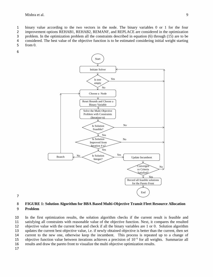
The solution methodology is presented in Figure 1.The first step is to initiate the solver to read the input 34 and look up for the binary variable indices with lower bound to 0 and upper bound to 1 for each binary 35 decision variable. Please note that the objective function consists of both TSWARL and NPC in the 36 proposed transit fleet resource allocation model. An important consideration needs to be given to the 37 overall objective function which cannot be a direct sum of both the objectives as it is possible that 38 magnitude of one objective may be very high compared to other. In classical weighted some approach this 39 is overcome by normalizing each objective function. The normalized objective function can be determined 40 by obtaining expectation of each objective function value divided by the expected value of the objective 41 function. The next step is to construct one empty node and create a tree by setting an initial value of 42 objective function. In the tree we try to solve for a node by setting the binary variable bounds, and fix 43

Mishra et al. 9

binary value according to the two vectors in the node. The binary variables 0 or 1 for the four 1 improvement options REHAB1, REHAB2, REMANF, and REPLACE are considered in the optimization 2 problem. In the optimization problem all the constraints described in equation (6) through (15) are to be 3 considered. The best value of the objective function is to be estimated considering initial weight starting 4 from 0. 5

6

7

FIGURE 1: Solution Algorithm for BBA Based Multi-Objective Transit Fleet Resource Allocation 8

Problem 9

In the first optimization results, the solution algorithm checks if the current result is feasible and 10 satisfying all constraints with reasonable value of the objective function. Next, it compares the resulted 11 objective value with the current best and check if all the binary variables are 1 or 0. Solution algorithm 12 updates the current best objective value, i.e. if newly obtained objective is better than the current, then set 13 current to the new one, otherwise keep the incumbent. This process is repeated up to a change of 14 objective function value between iterations achieves a precision of 10−6 for all weights. Summarize all 15 results and draw the pareto front to visualize the multi objective optimization results. 16 17

Initiate Solver

Is tree

empty

Choose a Node

Reset Bounds and Choose a

Binary Variable

Solve the Multi Objective

Problem with Constraints

(Iteration=n)

Is Solution

Feasible?

Update Incumbent

Is Solution

Improved from

Iteration # n?

Is Solution

Integer?Branch

Convergen

ce Criteria

Satisfied?

Start

End

YesNo

Yes

Yes

Yes

No

No

No

No

Yes

Record all feasible solutions

for the Pareto Front

Mishra et al. 10

6. Data 1

A Public Transportation Management System (PTMS) database developed by Michigan Department of 2 Transportation (MDOT) containing actual fleet data is used for the case study demonstration. The 3 distribution of the Remaining Life (RL) in years of the fleet for a few of the 93 agencies for the base year 4 (2002) is shown in Table 1. Only a fraction of the table is presented for brevity. Table 1 shows the 5 distribution of fleet size by their remaining life (RL) for each agency. For example, agency 1 has one bus 6 with zero years of RL, 2 buses with seven years of RL and so on, for a total fleet size of 3.The last row of 7 the table shows that the total fleet is of 720 buses, of which 235 buses have zero years of RL, and need 8 replacement. The last column of the Table 1 gives the weighted average remaining life (WARLi) for each 9 agency, computed from the distribution of RL for the agency. For example, the WARLi of the first 10 agency is calculated as (0x1+1x0+…+7x2)/3 =4.67. The base year total weighted average remaining life 11 of the entire fleet (TWARL) is 225.23 years. The following improvement options are used in the case 12 study: 13

• Replacement (REPLACE)—process of retiring an existing vehicle and procuring a completely 14 new vehicle. Buses proposed to be replaced using federal dollars are expected to be at the end of 15 their MNSLs, as described above. (Life expectancy: seven years) 16

• Rehabilitation (REHAB)—process by which an existing bus is rebuilt to the original 17 manufacturer’s specification. The focus of rehabilitation is on the vehicle interior and mechanical 18 systems, including rebuilding engines, transmission, brakes, and so on. Two types of 19 rehabilitation: REHAB1 and REHAB2 with moderate to higher levels of engine rebuilds are 20 considered in this study (Life expectancy: 2 to 3 years) 21

• Remanufacturing (REMANF)—process by which the structural integrity of the bus is restored to 22 original design standards. This includes remanufacturing the bus chassis as well as the drivetrain, 23 suspension system, steering components, engine, transmission, and differential with new and 24 manufactured components and a new bus body. ( Life Expectancy: 4 years) 25

• Further, it was assumed that a vehicle may be rehabilitated (REHAB1 or REHAB2) only up to 26 two consecutive terms, and then must be replaced (REPL) with a new bus. A vehicle with 27 REHAB1 and REHAB2 (or vice versa) in two consecutive terms also should be replaced. A 28 vehicle may be remanufactured (REMANF) only one time, and then must be replaced (REPL) 29 with a new bus. A vehicle rehabilitated (REHAB1 and REHAB2) once can be eligible for 30 remanufacturing (REMANF) before it is replaced (REPLACE). 31

TABLE 1 Base year distribution of remaining life (RL), fleet size, and weighted average of 32

remaining life of sample agencies before allocation of resources for the case study 33

Agency

Distribution of Remaining Life Total

Fleet

Size

WARLi

(years) 0 1 2 3 4 5 6 7

1 1 0 0 0 0 0 0 2 3 4.67

2 1 0 0 0 0 0 0 0 1 0

. . . . . . . . . . .

. . . . . . . . . . .

. . . . . . . . . . .

92 2 1 0 0 1 1 0 3 8 3.88

93 2 0 0 0 1 3 1 0 7 3.57

Total 235 122 44 23 63 77 78 78 720 225.23

Mishra et al. 11

7. Case Study Problem 1

The budgets available for each year and the unit cost for each improvement options for each year are 2

shown in Table 2. A seven year planning period is considered conforming to the MNSL requirement of 3

medium sized buses. Replacing all the 235 buses with zero years of RL (last row and second column of 4

Table 1) would require $19,161,900 (235 x $81,540) of investment which exceeds the first year budget. 5

Similarly, in the second year, 122 buses which had one year of RL in the base year will qualify for 6

improvement. 7

TABLE 2 Available Budget and Cost of Improvement Options 8

Year Budget Improvement Options and Costs

REPLACE

(X1= 7Years)

REHAB1

(X2= 2 Years)

REHAB2

(X3=3 Years)

REMANF

(X4= 4 Years)

2002 5,789,000 81,540 17,800 24,500 30,320

2003 9,130,000 81,540 17,800 24,500 30,320

2004 6,690,000 88,063 19,220 26,400 32,750

2005 5,200,000 88,063 19,220 26,400 32,750

2006 6,750,000 95,108 20,740 28,500 35,370

2007 6,600,000 95,108 20,740 28,500 35,370

2008 5,850,000 102,720 22,400 30,780 38,200

2009 6,680,000 102,720 22,400 30,780 38,200

Total 52,889,000

9

Replacing all these buses with remaining life 1 year would require $9,947,880 (122x$81,540), which also 10 exceeds the second year budget and so on for other years. Moreover, if the replacement process is 11 continued from year 2002 through 2009, when the buses reach their MNSL, it will cost $88,488,688 (i.e. 12 235*81,540+122*81,540+……+235*102,720) to maintain the fleet size of 720 buses throughout the 13 planning period. However the total available budget is only $52,889,000 (Table 2). Therefore, there is a 14 need for a mechanism to identify improvement options for each agency, so that the NPC is minimized 15 with a user defined TSWARL. The case study problem is solved using Premium Solver Platform (37-38). 16

8. Results and Discussion 17

The results from the proposed model are illustrated in the Table 3 . We can see the values for a set of 18 weights ranging from 0 to one (the value of ρ) for each objective function. If the weight is 0 the 19 formulation is equal to single objective minimization of NPC as an objective function; whereas, if the 20 weight is 1 it represents a case of maximization of TSWARL as the only objective. The weights in the 21 case study were choosen to represent as many possible points in the complete the solution space, hence 60 22 weights were generated between 0 and 1. Only a total of seven points (including the two extreme points) 23 are shown in Table 3. 24

TABLE 3 Best pareto optimal solutions along with their weights 25

REPLACE (X1)

(7 Years)

REHAB1 (X2)

(2 Years)

REHAB 2(X3)

(3 Years)

REMANF (X4)

(4 Years)

TSWARL NPC ($) Weight

(ρ) 424 391 77 63 2556.42 42,991,614 0.00 404 371 140 172 2520.38 45,102,062 0.03 401 356 141 164 2545.40 44,536,264 0.22 384 410 61 272 2636.52 45,213,129 0.27 452 368 41 144 2770.41 45,877,804 0.64 445 296 73 179 2768.73 45,868,090 0.92 456 321 23 183 2815.82 46,133,613 1.00

Mishra et al. 12

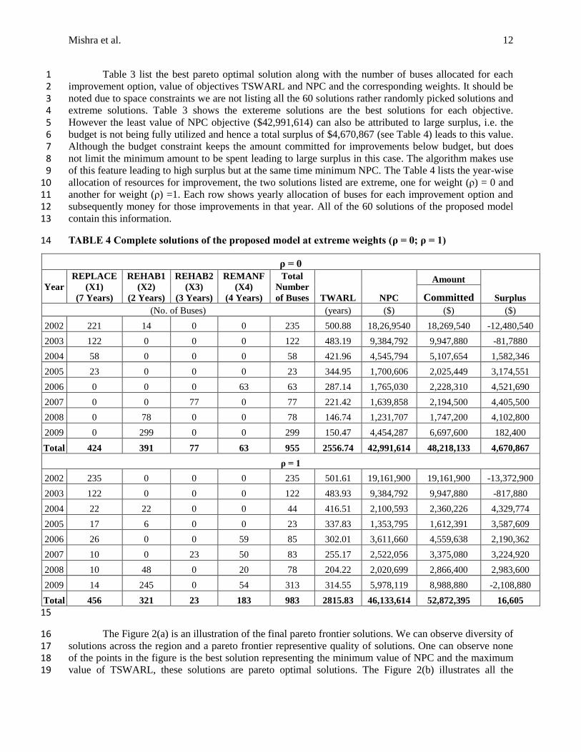
Table 3 list the best pareto optimal solution along with the number of buses allocated for each 1 improvement option, value of objectives TSWARL and NPC and the corresponding weights. It should be 2 noted due to space constraints we are not listing all the 60 solutions rather randomly picked solutions and 3 extreme solutions. Table 3 shows the extereme solutions are the best solutions for each objective. 4 However the least value of NPC objective ($42,991,614) can also be attributed to large surplus, i.e. the 5 budget is not being fully utilized and hence a total surplus of $4,670,867 (see Table 4) leads to this value. 6 Although the budget constraint keeps the amount committed for improvements below budget, but does 7 not limit the minimum amount to be spent leading to large surplus in this case. The algorithm makes use 8 of this feature leading to high surplus but at the same time minimum NPC. The Table 4 lists the year-wise 9 allocation of resources for improvement, the two solutions listed are extreme, one for weight (ρ) = 0 and 10 another for weight (ρ) =1. Each row shows yearly allocation of buses for each improvement option and 11 subsequently money for those improvements in that year. All of the 60 solutions of the proposed model 12 contain this information. 13

TABLE 4 Complete solutions of the proposed model at extreme weights (ρ = 0; ρ = 1) 14

15

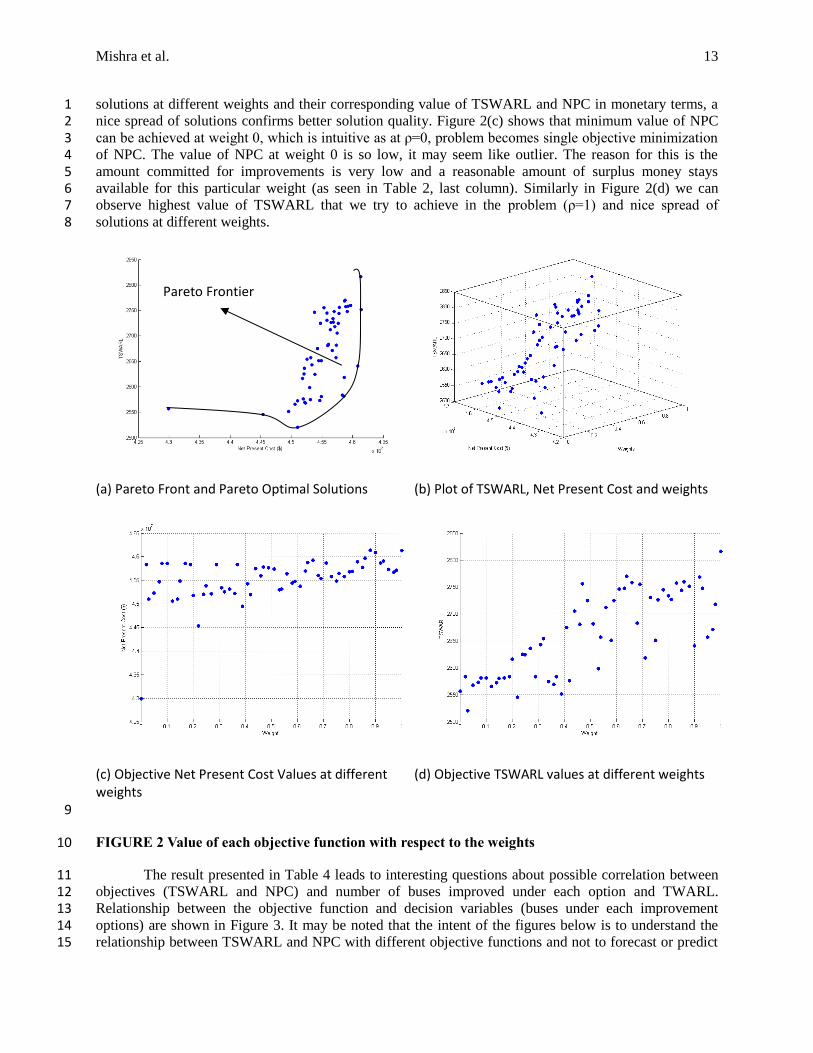
The Figure 2(a) is an illustration of the final pareto frontier solutions. We can observe diversity of 16 solutions across the region and a pareto frontier representive quality of solutions. One can observe none 17 of the points in the figure is the best solution representing the minimum value of NPC and the maximum 18 value of TSWARL, these solutions are pareto optimal solutions. The Figure 2(b) illustrates all the 19

ρ = 0

Year

REPLACE

(X1)

(7 Years)

REHAB1

(X2)

(2 Years)

REHAB2

(X3)

(3 Years)

REMANF

(X4)

(4 Years)

Total

Number

of Buses TWARL NPC

Amount

Surplus Committed

(No. of Buses) (years) ($) ($) ($)

2002 221 14 0 0 235 500.88 18,26,9540 18,269,540 -12,480,540

2003 122 0 0 0 122 483.19 9,384,792 9,947,880 -81,7880

2004 58 0 0 0 58 421.96 4,545,794 5,107,654 1,582,346

2005 23 0 0 0 23 344.95 1,700,606 2,025,449 3,174,551

2006 0 0 0 63 63 287.14 1,765,030 2,228,310 4,521,690

2007 0 0 77 0 77 221.42 1,639,858 2,194,500 4,405,500

2008 0 78 0 0 78 146.74 1,231,707 1,747,200 4,102,800

2009 0 299 0 0 299 150.47 4,454,287 6,697,600 182,400

Total 424 391 77 63 955 2556.74 42,991,614 48,218,133 4,670,867

ρ = 1

2002 235 0 0 0 235 501.61 19,161,900 19,161,900 -13,372,900

2003 122 0 0 0 122 483.93 9,384,792 9,947,880 -817,880

2004 22 22 0 0 44 416.51 2,100,593 2,360,226 4,329,774

2005 17 6 0 0 23 337.83 1,353,795 1,612,391 3,587,609

2006 26 0 0 59 85 302.01 3,611,660 4,559,638 2,190,362

2007 10 0 23 50 83 255.17 2,522,056 3,375,080 3,224,920

2008 10 48 0 20 78 204.22 2,020,699 2,866,400 2,983,600

2009 14 245 0 54 313 314.55 5,978,119 8,988,880 -2,108,880

Total 456 321 23 183 983 2815.83 46,133,614 52,872,395 16,605

Mishra et al. 13

solutions at different weights and their corresponding value of TSWARL and NPC in monetary terms, a 1 nice spread of solutions confirms better solution quality. Figure 2(c) shows that minimum value of NPC 2 can be achieved at weight 0, which is intuitive as at ρ=0, problem becomes single objective minimization 3 of NPC. The value of NPC at weight 0 is so low, it may seem like outlier. The reason for this is the 4 amount committed for improvements is very low and a reasonable amount of surplus money stays 5 available for this particular weight (as seen in Table 2, last column). Similarly in Figure 2(d) we can 6 observe highest value of TSWARL that we try to achieve in the problem (ρ=1) and nice spread of 7 solutions at different weights. 8

(a) Pareto Front and Pareto Optimal Solutions (b) Plot of TSWARL, Net Present Cost and weights

(c) Objective Net Present Cost Values at different weights

(d) Objective TSWARL values at different weights

9

FIGURE 2 Value of each objective function with respect to the weights 10

The result presented in Table 4 leads to interesting questions about possible correlation between 11 objectives (TSWARL and NPC) and number of buses improved under each option and TWARL. 12 Relationship between the objective function and decision variables (buses under each improvement 13 options) are shown in Figure 3. It may be noted that the intent of the figures below is to understand the 14 relationship between TSWARL and NPC with different objective functions and not to forecast or predict 15

Pareto Frontier

Mishra et al. 14

the results. The results shown in Figure 3 are not intended to be used as a substitute for optimization in 1 resource allocation problems rather has been shown to explore correlation. 2

Goodness of fit: SSE: 2.061e+005 R-square: 0.4087

Coefficients:

p1 = 49.15

p2 = 2660

Goodness of fit: SSE: 1.451e+005 R-square: 0.583

Coefficients:

p1 = -58.73

p2 = 2660

(a) Linear Relationship between TSWARL and Fleet for

Replacement (REPLACE) option in the planning period

(b) Linear Relationship between TSWARL and Fleet for

Rehabilitation (REHAB2) option in the planning period

Goodness of fit: SSE: 2.129e+005 R-square: 0.3895

Coefficients:

p1 =-47.97

p2 = 2660

Goodness of fit: SSE: 1.249e+013 R-square: 0.00047

Coefficients:

p1 = -1.005e+004

p2 = 4.553e+007

(c) Linear Relationship between TSWARL and Total

Fleet selected for all improvements in the planning

period

(d) Linear Relationship between NPC and Total Fleet

selected for all improvements in the planning period

3 FIGURE 3 Relationship of improvement options with objective functions during planning period for all 4 generated solutions in a linear polynomial form as f(x) = p1*x + p2 5 6 As can be observed from Figure 3, only a linear relation between TSWARL and REHAB2 option 7 has acceptable R-square value. Further, it is an inverse relationship, i.e. the higher the number of buses in 8 REHAB2, the lower the value of TSWARL. The relationship between TSWARL and REPLACE option 9 is a positive one, but it does not show a strong correlation. Similarly, there is a weak correlation between 10 TSWARL and Total Fleet for improvement, NPC, and REPLACE option (Figure 3 (d)). Other 11 comparisons are not listed, as the relationship betweeen decision variables and objective functions is 12

Mishra et al. 15

weak. It can be inferred that TSWARL is inversely impacted by buses going for rehabilitation for 3 years 1 and that is the reason we see very small number of buses allocated for rehabilitation (REHAB2) option in 2 the Table 4. In fact the key to maximizing TSWARL is to rehabilitate the least number of buses in the 3 fifth year. This further leads to question of exploring each year improvements along with the objective 4 function values. The Figure 4 (a-d) illustrates some insights in that direction. 5

Goodness of fit: SSE: 4.234e+004 R-square: 0.8785

Coefficients:

p1 = 72.05

p2 = 2660

Goodness of fit: SSE: 2.83e+005 R-square: 0.1884

Coefficients:

p1 =33.37

p2 =2660

a) Linear correlation between TSWARL and TWARL

in the year 2009

b) Linear correlation between TSWARL and TWARL in

the year 2008

Goodness of fit: SSE: 3.181e+005 R-square: 0.0876

Coefficients:

p1 = 22.76

p2 = 2660

Goodness of fit: SSE: 8.701e+012 R-square: 0.3039

Coefficients:

p1 = 2.537e+005

p2 = 4.553e+007

c) Linear correlation between TSWARL and TWARL

in the year 2007

d) Linear correlation between NPC and TWARL in the

year 2009

FIGURE 4 Relationship of TWARL for year 2009, 2008, 2007 with objective function values in a linear 6 polynomial form as f(x) = p1*x + p2 7

In the Figure 4(a), it can be observed that there is a strong correlation between TWARL for the 8 year 2009 and TSWARL. This implies that the fleet chosen for the improvement in the last year of 9 planning period significantly contributes to the high value of TSWARL. However, it should be observed 10 that the similar relationship does not hold for TWARL values for the years 2007, 2008, years (Figures 4b 11

Mishra et al. 16

and 4c) and for other years 2002-2006. Further, it is seen that the TWARL values do not have a 1 significant effect on the value of Net Present Cost. 2

Budget Sensitivity 3

To understand the budget sensitivity, multiple runs with different weights and lower budgets were 4 performed. It was observed that solver fails to obtain a solution without violating the budget constraints 5 below 13% of the original budget value $52,889,000. Therefore, in the Table 5, we present solutions 6 obtained at lower budget value $46,013,430 (13% reduction of $52,889,000) and the weights of ρ = 0, 0.5 7 and 1. It can be observed (Table 5) that at a lower budget, the algorithm chooses lower cost, and medium 8 age improvement options (REHAB2 and REMANF) to achieve the minimum NPC value. At the original 9 budget and for similar weight, the algorithm prefers extreme improvement options (REHAB1 and 10 REPLACE) with higher cost and longer life (better quality). Another interesting observation is for ρ = 1 11 (Maximization of TSWARL), the total number of buses for improvement between year 2002-2005 12 remains the same at both the budget levels (Table 4 and 5). The difference starts to appear after year 2006 13 where the model tries to adjust for the budget. 14

9. Synthesis of Results 15

The multi objective optimization approach presented for the transit resource allocation resulted in a pareto 16 optimial solutions demostrating trade off between NPC and TSWARL. The optimization results show that 17 appropriate improvement options can be choosen to achieve a specific objective function. The 18 relationship between NPC and TSWARL is non-linear in nature because of the incorporation of the 19 interest factors in computing NPC. When NPC is compared with individual year quality measure 20 (TWARL), it is observed that initially, TWARL remains relatively constant with increase in NPC up to a 21 certain point, beyond which TWARL increases in the later years. In all the solutions, a relationship 22 between replacement (REPLACE) option and rehabilitation option (REHAB2) with TSWARL has been 23 consistently observed. However, the relationship between TSWARL and REHAB2 is inversely 24 proportional but strongly correlated. This represents the fleet size chosen for this improvement governs 25 the overall objective of TSWARL. 26

The relationship between TSWARL and TWARL in the year 2009 is very strongly correlated 27 compared to any other relationship between decision variables and objectives. Thus suggesting that the 28 last year’s total expected weighted remaining life plays an important role in maximizing the TSWARL 29 objective. A limitation of the formulation is that minimum NPC can be achieved by investing relatively 30 less in the improvements and obtaining alarge surplus (reducing expenditure from budget) as the 31 constraint is to spend less than a particular budget value. This can be overcome by adding a constraint on 32 minimum spending amount. A sensitivity analysis for a lower budget shows efficacy of the model to work 33 at 13 percent lower than original budget and obtain results. A comparison between low budget and exact 34 budget cases show variation in fleet selection for each improvement option under different budget levels. 35

Computational Effort 36

The average computational time to solve this problem for a single weight using the PSP solver platform 37 (37;38) is two minutes in a Windows 7 64 bit operating system, on i7 Quad Core Processor and 6 GB 38 RAM. The overall time taken to obtain the all the 60 solutions is approximately two hours. 39

40

41

42

43

Mishra et al. 17

TABLE 5 Complete solutions of the proposed model at lower budget and weights (ρ=0; ρ=0.5; ρ=1) 1

2

ρ = 0 (Budget=$46,013,430)

Year

REPLACE

(X1)

(7 Years)

REHAB1

(X2)

(2 Years)

REHAB2 (X3)

(3 Years)

REMANF

(X4)

(4 Years)

Total

Number

of Buses TWARL NPC

Amount

Surplus Committed

(No. of Buses) (years) ($) ($) ($)

2002 166 62 7 0 235 450.28 14810740 14810740 -9021740

2003 40 0 82 0 122 418.47 4972264 5270600 3859400

2004 86 2 18 0 106 388.92 7197453 8087058 -1397058

2005 12 11 7 0 30 345.58 1219947 1452976 3747024

2006 1 0 0 146 147 305.32 4165722 5259128 1490872

2007 1 0 102 3 106 251.78 2322641 3108218 3491782

2008 0 85 0 0 85 178.42 1342245 1904000 3946000

2009 0 243 0 1 244 161.52 3645444 5481400 1398600

Total 306 403 216 150 1075 2500.29 39,676,456 45,374,120 7,514,880

ρ = 0.5 (Budget=$46,013,430)

2002 235 0 0 0 235 501.61 19161900 19161900 -1.3E+07

2003 122 0 0 0 122 483.93 9384792 9947880 -817880

2004 44 0 0 0 44 421.66 3448533 3874772 2815228

2005 15 0 8 0 23 342.43 1286418 1532145 3667855

2006 0 0 0 63 63 284.62 1765030 2228310 4521690

2007 0 0 77 0 77 218.90 1639858 2194500 4405500

2008 0 86 0 0 86 145.33 1358036 1926400 3923600

2009 0 230 0 0 230 115.92 3426374 5152000 1728000

Total 416 316 85 63 880 2514.41 41,470,943 46,017,907 6,871,093

ρ = 1 (Budget=$46,013,430)

2002 235 0 0 0 235 501.61 19161900 19161900 -1.3E+07

2003 122 0 0 0 122 483.93 9384792 9947880 -817880

2004 44 0 0 0 44 421.66 3448533 3874772 2815228

2005 22 0 1 0 23 344.15 1648833 1963786 3236214

2006 0 0 0 63 63 286.35 1765030 2228310 4521690

2007 0 0 77 0 77 220.63 1639858 2194500 4405500

2008 0 79 0 0 79 146.20 1247498 1769600 4080400

2009 0 265 0 0 265 135.16 3947779 5936000 944000

Total 423 344 78 63 908 2539.68 42,244,224 47,076,748 5,812,252

Mishra et al. 18

1

10. Conclusion 2

A novel multi-objective optimization model for transit fleet resource allocation is proposed in this paper. 3 Two conflicting objectives, maximization of TSWARL and minimization of NPC are used. TSWARL is a 4 quality measure represents remaining life of the transit fleet that the agency would like to maximize. 5 Further, it is equally important to determine the cost required to achieve a certain TSWARL, this in terms 6 of present value of the cost can be referred to NPC. It being an expenditure measure the transit agency 7 would like to minimize NPC, a premise that conflicts with maximizing TSWARL. In the single objective 8 optimization problem either TSWARL or NPC can be analyzed only one at a time. Further, while 9 analyzing TSWARL the single objective optimization problem is blind to the NPC, and vice versa; as 10 each is assumed as a by-product of other. The proposed multiobjective optimization problem has the 11 advantage of considering both objectives simultaneously and provides a series of solutions as a trade-off 12 for the decision maker. Branch and bound algorithm (BBA) is used to solve the multi-objective 13 formulation since it results in better optimal solutions compared to GA for such problems. The transit 14 fleet data over an eight year period from the Michigan Department of Transportation is used as the case 15 study. As per FTA standards, four improvement options are used to allocate the fleet approaching MNSL. 16

The multi objective transit fleet resource allocation model has multiple dimensions of significant 17 contribution to research and practice. First, the proposed model provides a trade-off between two 18 objectives TSWARL, the quality measure and NPC, the cost measure. An analysis of this trade-off has 19 not been attempted in literature. Second, solutions to both objectives in a multi-year planning period 20 provide the decision makers with multiple options. Third, the proposed method allows the decision 21 makers to explore the trade-off solutions between the conflicting objectives like TSWARL and NPC to 22 make an informed decision. The research in transit resource allocation can be further enhanced in several 23 ways. The classical technique of weighted sum approach presented in the paper has been extensively 24 applied in multi-objective optimization research and practice. However, recent advancement of 25 evolutionary approaches for solving multi-objective optimization can be considered in future research. 26 The case study demonstrated in the paper is for the medium duty, medium sized transit fleet system in 27 Michigan. The methodology can be applied to different fleet age types, policy, and budget constraints. 28 Another factor is fleet uncertainty because of bus breakdown, accidents or other events, that can be 29 modeled into the problem to build a robust fleet resource allocation. 30

11. References 31

1. FTA. (2006a). “Public Transportation in the U.S.: Performance and Condition.” Federal Transit 32 Administration, A Report To Congress Volume 49, Chapter 53, Section 5307. 33

2. FTA. (2006b). “Public Transportation in the U.S.: Performance and Condition.” Federal Transit 34 Administration, A Report To Congress Volume 49, Chapter 53, Section 5302. 35

3. Mishra, S., Mathew, T. V., and Khasnabis, S. (2010). Single Stage Integer Programming Model 36 for Long Term Transit Fleet Resource Allocation, in Journal of Transportation Engineering, 37 American Society of Civil Engineers (ASCE), vol. 136(4). pp. 281-290. 38

4. Mathew, T.V., Khasnabis, S. and Mishra, S. 2010. Optimal resource allocation among transit 39 agencies for fleet management. Transportation Research Part A: Policy and Practice, 44(6), 40 pp.418–432. 41

5. Sharma, S., and Mathew, T. V. (2011) Multi-objective network design for emission and travel-42 time trade-off for a sustainable large urban transportation network, Environment and Planning B: 43 Planning and Design38, 520–538. 44

6. Blazer, B. B., Savage A. E., and Stark, R. C. (1980). “Survey and Analysis of Bus Rehabilitation 45 in the Mass Transportation Industry.” ATE Management and Service Company, Cincinnati, Ohio. 46

Mishra et al. 19

7. Bridgeman, M. S., Sveinsson, H., and King, R. D. (1983)“Economic Comparison of New Buses 1 Versus Rehabilitated Buses”. Battelle Columbus Laboratories, Columbus, Ohio. Prepared for 2 Urban Mass Transportation Administration, Washington, D.C. 3

8. ATE. (1983). “Vehicle Rehabilitation/ Replacement Study.” ATE Management Services & 4 Enterprises, Prepared for Urban Mass Transportation Administration, Washington, D.C. 5

9. Bridgman, M. S., McInerney, S. R., Judnick, W. E., Artson, M., and Fowler, B.(1984). 6 “Feasibility of Determining Economic Differences Between New Buses and Rehab 7 Buses.”UMTA-IT-06-0219-034. Battelle Columbus Laboratories, Columbus, Ohio 8

10. Foerster, J.F., 1985. Bus maintenance cost control. In Proceedings of a Specialty Conference: 9 Innovative Strategies to Improve Urban Transportation Performance. Knoxville, TN, Belgium, 10 pp. 54–66. 11

11. Giuliani, C., 1987. Bus-inspection guidelines. Final report, 12 12. Pake, B.E., 1985. Evaluation of Bus Maintenance Operations. In Transportation Research Record 13

N1019. TRIS, TRB, pp. 77–84. 14 13. Drake, R.W., 1985. Evaluation of Bus Maintenance Manpower Utilization. In Transportation 15

Research Board, pp. 49–62. Available at: http://www.trb.org/Publications/Pages/262.aspx 16 14. Pake, B.E., 1986. Application of a Transit Maintenance Management Evaluation Procedure. In 17

Transportation Research Board, pp. 13–21. Available at: 18 http://www.trb.org/Publications/Pages/262.aspx. 19

15. Dutta, U.and Maze, T.H., 1989. Model for comparing performance of various transit maintenance 20 repair policies. Journal of Transportation Engineering, 115(4), pp.450-457. 21

16. Maze, T.H., 1987.Theory and Practice of Transit Bus Maintenance Performance Measurement. In 22 Transportation Research Board, pp. 18–29. Available at: http://worldcat.org/isbn/0309046513. 23

17. Jakubowski, A. and Kulikowski, R., 1996. A decision support approach for R and D resource 24 allocation. In Proceedings of 13th European Meeting on Cybernetics and Systems Research. 25 Vienna, Austria, pp. 715–718. 26

18. Ross, A.D., 2000. Performance-based strategic resource allocation in supply networks. 27 International Journal of Production Economics, 63(3), pp.255–266. 28

19. Basso, A.and Peccati, L.A., 2001.Optimal resource allocation with minimum activation levels and 29 fixed costs. European Journal of Operational Research, 131(3), pp.536–549. 30

20. Bokhorst, J.A.C., Slomp, J. and Suresh, N.C., 2002. An integrated model for part-operation 31 allocation and investments in CNC technology. International Journal of Production Economics, 32 75(3), pp.267–285. 33

21. Gratcheva, E.M. and Falk, J.E., 2003. Optimal deviations from an asset allocation. Computers 34 and Operations Research, 30(11), pp.1643–1659. 35

22. Sheu, J.-B., 2006.A novel dynamic resource allocation model for demand-responsive city 36 logistics distribution operations. Transportation Research Part E: Logistics and Transportation 37 Review, 42(6), pp.445–472. 38

23. Karlaftis, M.D., Kepaptsoglou, K.L. and Lambropoulos, S., 2007. Fund Allocation for 39 Transportation Network Recovery Following Natural Disasters, pp.82–89. 40

24. Allen Jr, W.G. and DiCesare, F., 1976. Transit Service evaluation: preliminary identification of 41 variables characterizing level of service. Transportation Research Record, (606). 42

25. Marshment, R.S., 1993. Establishing national priorities for rail transit investments. Policy Studies 43 Journal, 21(2), pp.338–346. 44

26. Spasovic, L.N., Boile, M.P. and Bladikas, A.K., 1994. Bus transit service coverage for maximum 45 profit and social welfare. Transportation Research Record, (1451). 46

27. Chu, X. and Polzin, S., 1998.Considering build-later as an alternative in major transit investment 47 analyses. Transportation Research Record: Journal of the Transportation Research Board, 48 1623(-1), pp.179–184. 49

Mishra et al. 20

28. Ghandforoush, P., Collura, J. and Plotnikov, V., 2003.Developing a Decision Support System for 1 Evaluating an Investment in Fare Collection Systems in Transit. Journal of Public 2 Transportation, 6(2), pp.61–86. 3

29. Naesun, P., Yoon, H.R. and Hitoshi, I., 2003. The feasibility study on the new transit system 4 implementation to the congested area in Seoul. Journal of the Eastern Asia Society for 5 Transportation Studies, 5. 6

30. Litvinenko, M. and Palšaitis, R., 2006. The evaluation of transit transport probable effects on the 7 development of country’s economy. Transport, 21(2), pp.135–140. 8

31. Raju, S., 2008. Project NPV, Positive Externalities, Social Cost-Benefit Analysis-The Kansas 9 City Light Rail Project. Journal of Public Transportation, 11(4). 10

32. Chow, J.Y.J. and Regan, A.C., 2011. Network-based real option models. Transportation 11 Research Part B: Methodological, 45(4), pp.682–695. 12

33. Deng, Lianbo, Qiang Zeng, Wei Gao, and Zhao Zhou. 2011. “Optimization Method for Train 13 Plan of Urban Rail Transit.” In 11th International Conference of Chinese Transportation 14 Professionals: Towards Sustainable Transportation Systems, American Society of Civil Engineers 15 (ASCE). doi:10.1061/41186(421)117. http://dx.doi.org/10.1061/41186(421)117. 16

34. Desai, Chirag, Florence Berthold, and Sheldon S. Williamson. 2010. “Optimal Drivetrain 17 Component Sizing for a Plug-in Hybrid Electric Transit Bus Using Multi-objective Genetic 18 Algorithm.” In 4th IEEE Electrical Power and Energy Conference: 19 doi:10.1109/EPEC.2010.5697242. http://dx.doi.org/10.1109/EPEC.2010.5697242. 20

35. Mauttone, Antonio, and Maria E. Urquhart. 2009. “A Multi-objective Metaheuristic Approach for 21 the Transit Network Design Problem.” Public Transport 1 (4): 253–273. doi:10.1007/s12469-010-22 0016-7. 23

36. Wu, Wanyang, Albert Gan, Fabian Cevallos, and Mohammed Hadi. 2011. “Multiobjective 24 Optimization Model for Prioritizing Transit Stops for ADA Improvements.” Journal of 25 Transportation Engineering 137 (8): 580–588. doi:10.1061/(ASCE)TE.1943-5436.0000244. 26

37. PSP, 2011a.Premium Solver Platform, USA: Frontline Systems. 27 38. PSP, 2011b.Premium Solver Platform-Solver Engines, USA: Frontline Systems. 28