Embed Size (px)
Citation preview

A multi-factor jump-diffusion
model for Commodities
John Crosby
7th October 2005
Seminar at the University Finance
Seminar, Cambridge University

Acknowledgements
• We thank Simon Babbs and Farshid
Jamshidian for comments which have
significantly enhanced our work. We also
thank Peter Carr, Darrell Duffie, Stewart
Hodges, Andrew Johnson, Daryl Mcarthur,
Anthony Neuberger and Nick Webber.
Introducing a multi-factor jump-
diffusion model for commodities
This presentation draws on my papers “A
multi-factor jump-diffusion model for
Commodities” and “Pricing commodity
options in a multi-factor jump-diffusion
model using Fourier Transforms”
(submitted for publication).

Empirical observations on the
commodities markets 1
• Spot commodity prices exhibit mean reversion.
• Futures (and forward) commodity prices have instantaneous volatilities which usually (not always) decline with increasing tenor.
• Jumps are somewhat more common and certainly much larger in magnitude than in other markets (eg equities or fx).
Empirical observations on the
commodities markets 2
• A common feature in commodities (esp.
Gas and Electricity) is that when there is a
jump, the spot and short-dated futures (or
forward) prices jump by a large amount but
long-dated contracts hardly jump at all (to
our knowledge no existing models have
accounted for this feature).
• Convenience yields are usually highly
volatile.
Commodities• Now let’s start to look at our model.
• We would like to capture the stylised
empirical features of the commodities
which we have just noted.
• We want a no-arbitrage model which
automatically fits the initial term structure
of futures (or forward) commodity prices.
Key Assumptions• We assume the market is frictionless, (ie no
bid-offer spreads, continuous trading is
possible, etc) and arbitrage-free.
• No arbitrage => existence of an equivalent
martingale measure (EMM).
• In this talk, we work exclusively under the
(or a) EMM.

Spot commodity prices
• We denote the value of the commodity at
time by . We define today to be
time and the value of the commodity
today is .
• (Value of the commodity means “spot
price” but in some markets spot is hard to
define).
0tC
t tC
0t

Spot commodity prices
• We do NOT assume that the spot is
tradeable (except as the deliverable on a
futures contract at maturity).
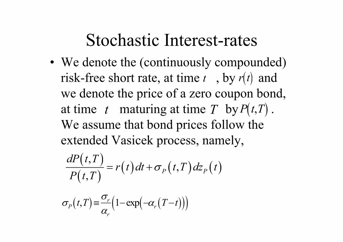
Stochastic Interest-rates
• We denote the (continuously compounded)
risk-free short rate, at time , by and
we denote the price of a zero coupon bond,
at time maturing at time by .
We assume that bond prices follow the
extended Vasicek process, namely,
( )( )
( ) ( ) ( ),
,,
P P
dP t Tr t dt t T dz t
P t Tσ= +
( ) ( )( )( ), 1 exprP r
r
t T T tσ
σ αα
≡ − − −
t ( )r t
t T ( ),P t T

• where and are positive constants.
• Define the state variable:
• ETS can write and in terms of
rσ rα
( ) ( )( ) ( )0
exp
t
P r r P
t
X t t s dz sσ α= − −∫
( )r t ( ),P t T
( )PX t

The model
• Let us denote the futures commodity price
at time for delivery at time by
• We take as given our initial (ie at time )
term structure of futures commodity prices.
• In the absence of arbitrage,
• Futures prices are martingales under the
EMM. (Cox et al. (1981)).
0t
t T ( ),H t T
( ),tC H t t=
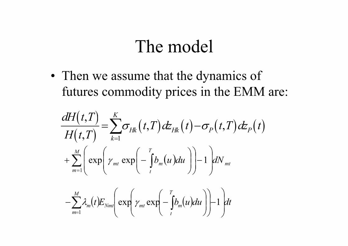
The model
• Then we assume that the dynamics of
futures commodity prices in the EMM are:
( )( )
( ) ( ) ( ) ( )1
,, ,
,
K
Hk Hk P P
k
dH t Tt T dz t t T dz t
H t Tσ σ
=
= −∑
( )∑ ∫=
−
−+
M
m
mt
T
t
mmt dNduub1
1expexp γ
( ) ( ) dtduubEt
T
t
mmtNmt
M
m
m
−
−− ∫∑
=
1expexp1
γλ
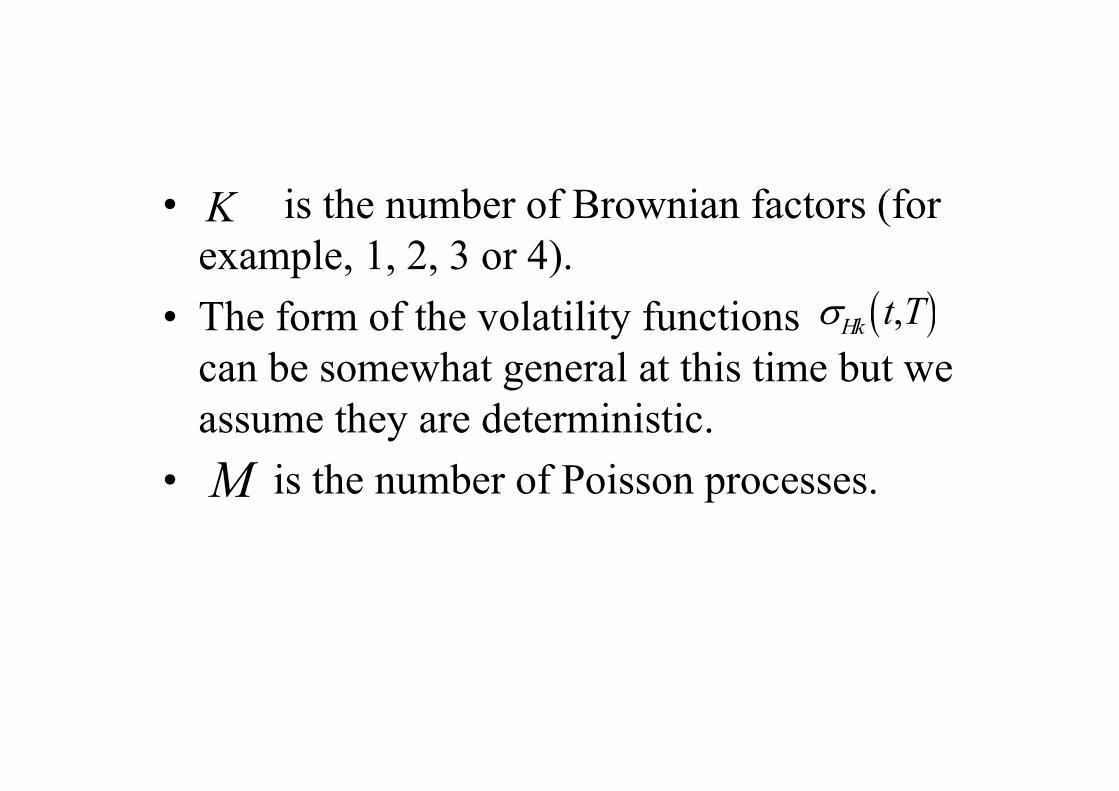
• is the number of Brownian factors (for
example, 1, 2, 3 or 4).
• The form of the volatility functions
can be somewhat general at this time but we
assume they are deterministic.
• is the number of Poisson processes.
K
( ),Hk t Tσ
M

• For each , , denotes
standard Brownian increments. We denote the
correlation (assumed constant) between
and by , for each , and the
correlation (assumed constant) between
and by for each and .
• if
k 1,2,...,k K= ( )Hkdz t
( )Hkdz t
( )Pdz t
PHkρ k( )Hkdz t
( )Hjdz tHkHjρ jk
1HkHjρ = k j=

Jump processes
• For each , , are
the (assumed) deterministic intensity rates
of the Poisson processes.
• for each are non-negative
deterministic functions. We call these the
jump decay coefficient functions.
• are the spot jump amplitudes.
m Mm ,...,1= ( )tmλ
( )ubm m
mtγ
M
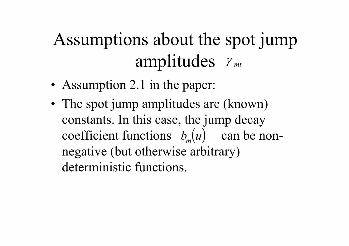
Assumptions about the spot jump
amplitudes
• Assumption 2.1 in the paper:
• The spot jump amplitudes are (known)
constants. In this case, the jump decay
coefficient functions can be non-
negative (but otherwise arbitrary)
deterministic functions.
mtγ
( )ubm
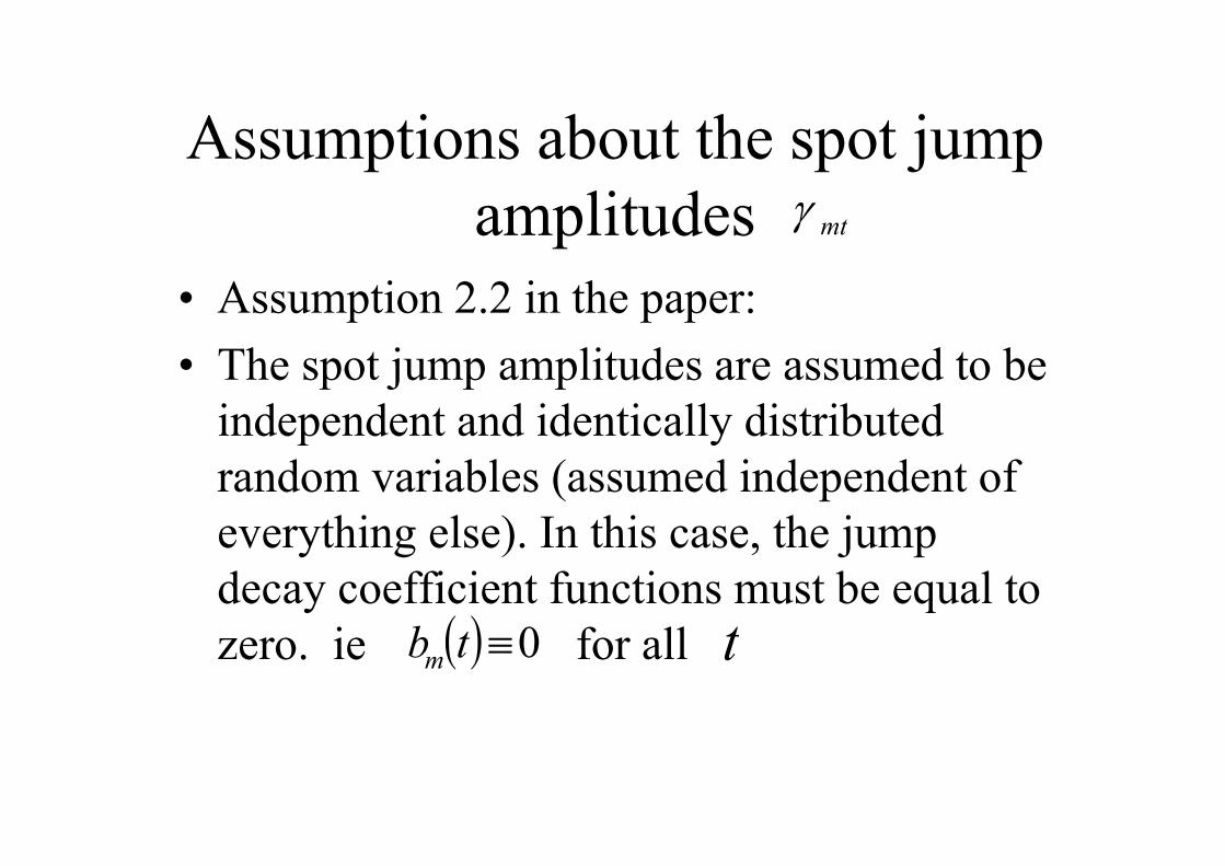
Assumptions about the spot jump
amplitudes
• Assumption 2.2 in the paper:
• The spot jump amplitudes are assumed to be
independent and identically distributed
random variables (assumed independent of
everything else). In this case, the jump
decay coefficient functions must be equal to
zero. ie for all
mtγ
( ) 0≡tbm t
Multiple Poisson processes
• All satisfy either Assumption 2.1 or 2.2
• But, if we have more than one Poisson
process, we can mix the assumptions
• Eg if 4 Poisson processes, we could have eg
3 satisfying assumption 2.1 and 1 satisfying
Assumption 2.2

Implications for completeness
• If all spot jump amplitudes are constants
(assumption 2.1) (and there are a sufficient
number of futures contracts of different
maturities), then the market is complete
(and hence the EMM is unique).
• Else the market is not complete (EMM not
unique but assume “fixed” by the market).
Implications for arbitrage
• It is not wholly obvious but the assumption
of no-arbitrage requires a condition
(analogous to the HJM drift condition). This
in turn, means we assume random jump
amplitudes (assumption 2.2) have an extra
condition ie
• Bjork, Kabanov and Runggaldier (1997)
• Crosby (2005)
( ) 0≡tbm
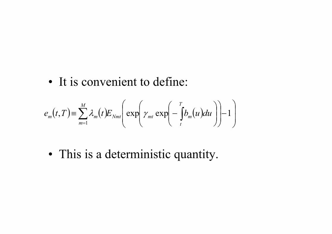
• It is convenient to define:
• This is a deterministic quantity.
( ) ( ) ( )
−
−≡ ∫∑
=
1expexp,1
T
t
mmtNmt
M
m
mm duubEtTte γλ
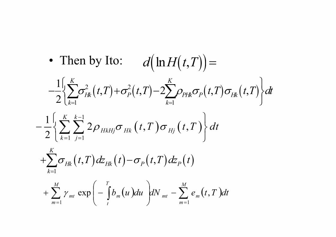
• Then by Ito:
( ) ( ) ( ) ( )2 2
1 1
1, , 2 , ,
2
K K
Hk P PHk P Hk
k k
t T t T t T t T dtσ σ ρ σ σ= =
− + −
∑ ∑
( ) ( )1
1 1
12 , ,
2
K k
HkHj Hk Hj
k j
t T t T dtρ σ σ−
= =
−
∑∑
( ) ( ) ( ) ( )1
, ,K
Hk Hk P P
k
t T dz t t T dz tσ σ=
+ −∑
( )( )ln ,d H t T =
( ) ( )∑∑ ∫==
−
−+
M
m
mmt
M
m
T
t
mmt dtTtedNduub11
,expγ
Implications
• Gas, Electricity: Short end of futures curve
jumps a lot, long end hardly jumps at all
(existing models do not seem to have this).
• Gold: Jumps are less of a feature (but they
do happen).
• “Gold trades somewhat like a currency”.
• ie jumps cause parallel shift in futures (and
forward) curve.
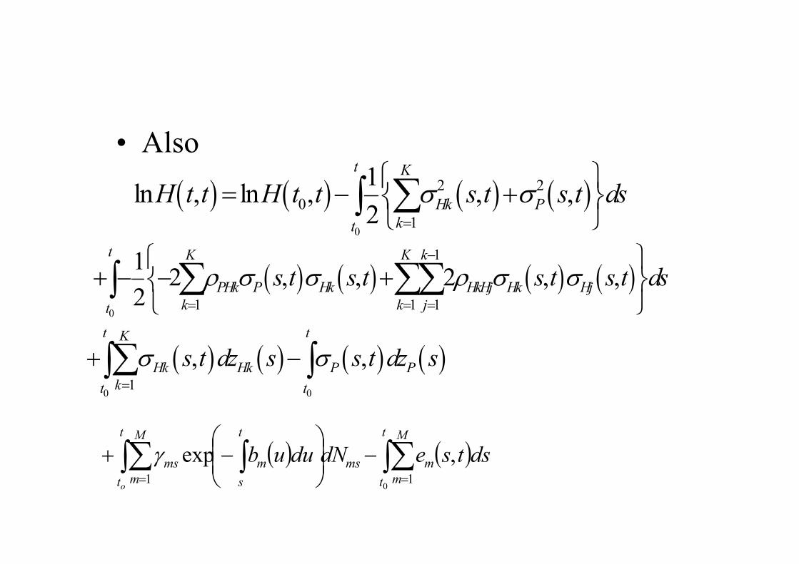
• Also
( ) ( ) ( ) ( )0
2 2
0
1
1ln , ln , , ,
2
t K
Hk P
kt
H t t H t t s t s t dsσ σ=
= − +
∑∫
( ) ( ) ( ) ( )0
1
1 1 1
12 , , 2 , ,
2
t K K k
PHk P Hk HkHj Hk Hj
k k jt
s t s t s t s t dsρ σ σ ρ σ σ−
= = =
+ − − +
∑ ∑∑∫
( ) ( ) ( ) ( )0 0
1
, ,
t tK
Hk Hk P P
kt t
s t dz s s t dz sσ σ=
+ −∑∫ ∫
( ) ( )∫∑∫∑ ∫==
−
−+
t
t
M
m
mms
t
t
M
m
t
s
mms dstsedNduub
o 011
,expγ
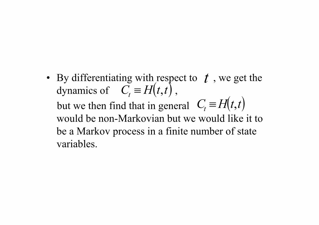
• By differentiating with respect to , we get the
dynamics of ,
but we then find that in general
would be non-Markovian but we would like it to
be a Markov process in a finite number of state
variables.
( )ttHCt ,≡t
( )ttHCt ,≡

• We consider the functional form for the
volatilities:
where , and
are deterministic functions.
Why?
( ) ( ) ( ) ( ), exp
t
Hk Hk Hk Hk
s
s t s s a u duσ η χ
= + − ∫
( )Hk sη ( )Hk sχ ( )Hka u

Gaussian state variables:
• Define the state variables:
• And for each
( ) ( )0
t
P r P
t
Y t dz sσ= ∫
( ) ( ) ( ) ( ) ( )0
0 0
exp exp
tt t
Hk Hk Hk Hk Hk
t t s
X t a u du s a u du dz sχ
= − − ∫ ∫ ∫
( ) ( ) ( )0
t
Hk Hk Hk
t
Y t s dz sη= ∫
k Kk ,...,2,1=
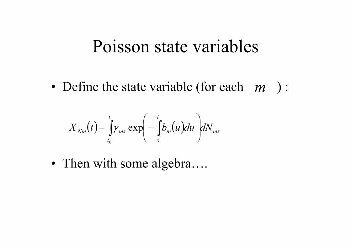
Poisson state variables
• Define the state variable (for each ) :
• Then with some algebra….
m
( ) ( )∫ ∫
−=
t
t
ms
t
s
mmsNm dNduubtX
0
expγ
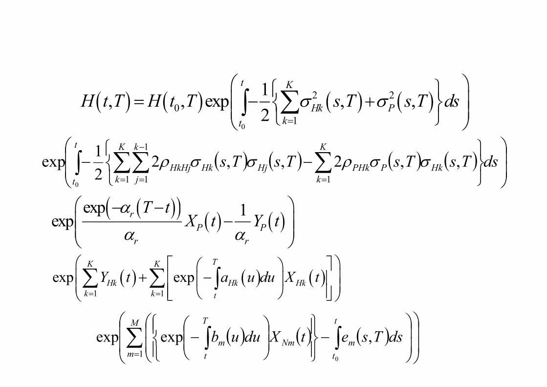
• We have the following expression for the
futures commodity price at time to
time in terms of the initial (ie at time )
futures commodity price and the state
variables:
( ),H t T t
T 0t
( ) ( ) ( ) ( )0
2 2
0
1
1, , exp , ,
2
t K
Hk P
kt
H t T H t T s T s T dsσ σ=
= − +
∑∫
( ) ( ) ( )1 1
exp exp
TK K
Hk Hk Hk
k k t
Y t a u du X t= =
+ −
∑ ∑ ∫
( )( )( ) ( )
exp 1exp
r
P P
r r
T tX t Y t
α
α α
− −−
( ) ( ) ( ) ( )
−−∫ ∑ ∑∑= =
−
=
dsTsTsTsTs
t
t
K
k
K
k
HkPPHk
k
j
HjHkHkHj
01 1
1
1
,,2,,22
1exp σσρσσρ
( ) ( ) ( )
−
−∑ ∫∫
=
M
m
t
t
mNm
T
t
m dsTsetXduub1
0
,expexp

Convenience Yields
• We show in the paper that:
• Our model automatically generates stochastic
convenience yields.
• The convenience yields also exhibit jumps, except in
the special case that for all
• We do not need to make any assumptions about the
stochastic process for convenience yields or its
market price of risk.
( ) 0≡tbm m

Mean reversion in spot
commodity prices
• In the paper, we show that the value of the
commodity ie follows a mean-
reverting jump-diffusion process.
• We also show how the jump decay coefficient
functions , if they are non-zero (ie
assumption 2.1 only), can also contribute to the
mean reversion effect.
• Jump decay coefficient functions analogous to
mean reversion rates.
( )ttHCt ,≡
( )tbm
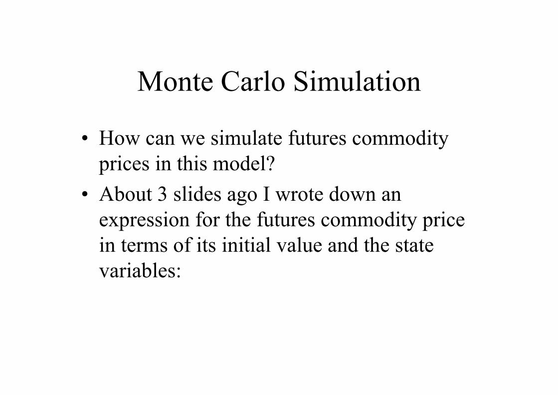
Monte Carlo Simulation
• How can we simulate futures commodity
prices in this model?
• About 3 slides ago I wrote down an
expression for the futures commodity price
in terms of its initial value and the state
variables:
( ) ( ) ( ) ( )0
2 2
0
1
1, , exp , ,
2
t K
Hk P
kt
H t T H t T s T s T dsσ σ=
= − +
∑∫
( ) ( ) ( ) ( )
−−∫ ∑ ∑∑= =
−
=
dsTsTsTsTs
t
t
K
k
K
k
HkPPHk
k
j
HjHkHkHj
01 1
1
1
,,2,,22
1exp σσρσσρ
( )( )( ) ( )
exp 1exp
r
P P
r r
T tX t Y t
α
α α
− −−
( ) ( ) ( )
1 1
exp exp
TK K
Hk Hk Hk
k k t
Y t a u du X t= =
+ −
∑ ∑ ∫
( ) ( ) ( )
−
−∑ ∫∫
=
M
m
t
t
mNm
T
t
m dsTsetXduub1
0
,expexp

Monte Carlo Simulation
• Therefore, we can easily do Monte Carlo
simulation if we can simulate the state
variables:
• Gaussian state variables are straightforward.
• So lets focus on the Poisson state variables.
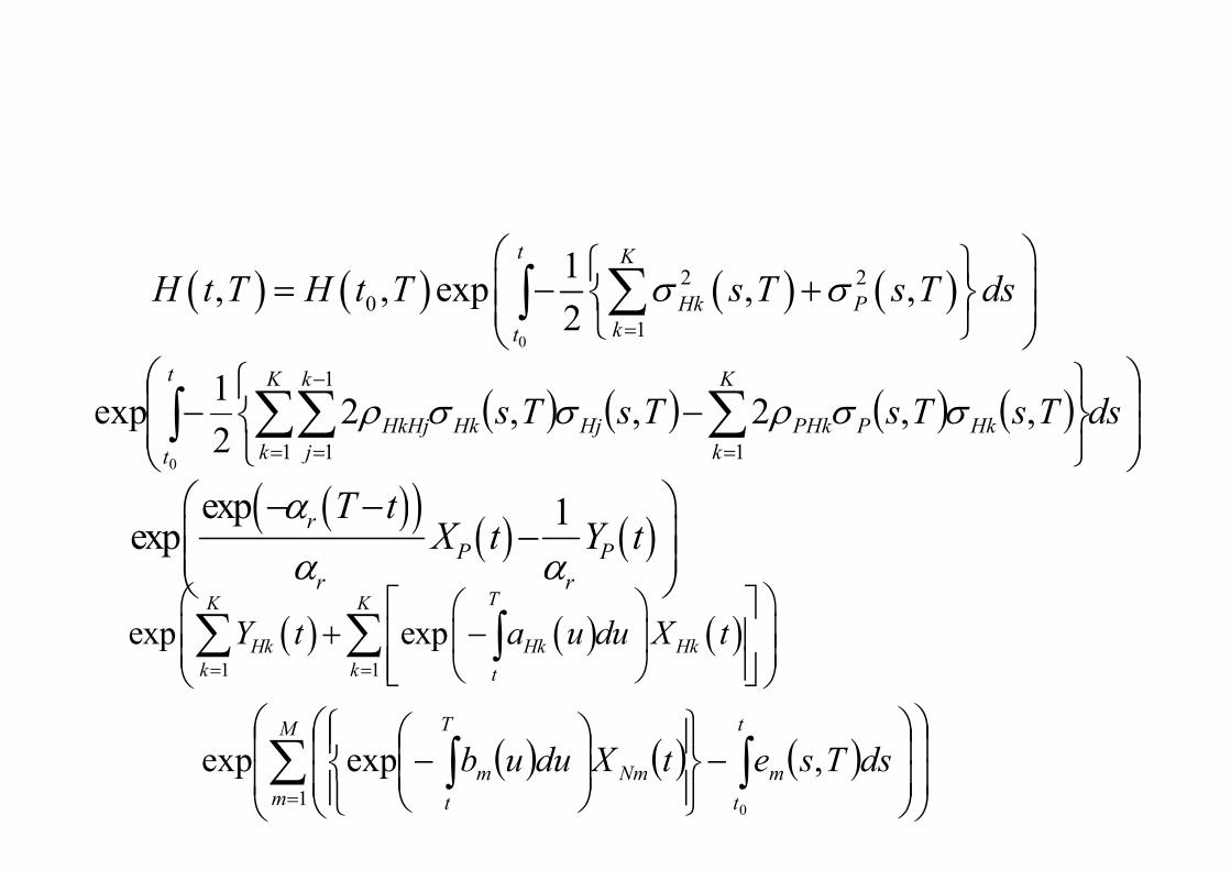
Poisson
• By definition, the probability that
there are jumps on the Poisson
Process in the time period to
is:
( ) ( )( )
!exp;,
0
0
0
m
nt
t
mt
t
mmmn
duu
duunttQ
m
−=
∫∫
λ
λ
( )mm nttQ ;,0mn
mtN 0t t

• We also need the following result (an
extension of a result in Karlin and Taylor
(1975) “A first course in stochastic
processes”):

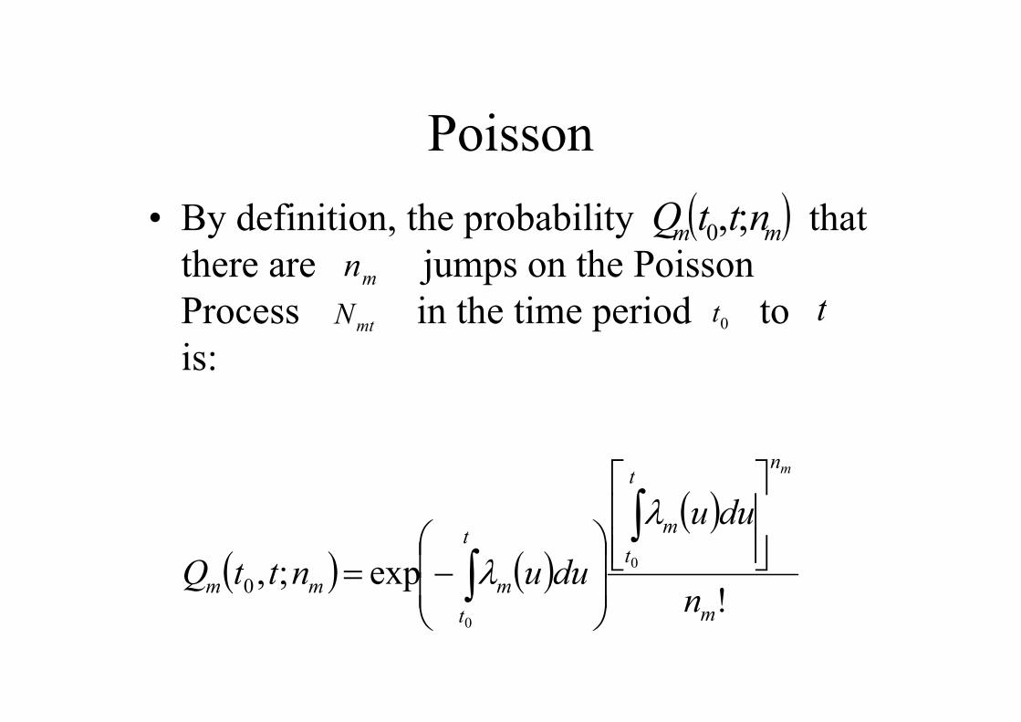
Proposition
• Suppose that we know that there have been
jumps between time and time .
Write the arrival times of the jumps as
. The conditional joint
density function of the arrival times, when
the arrival times are viewed as unordered
random variables, conditional on is:
mn 0t t
mnmm mSSS ,...,, 21
mmt nN =
( )===== mmtmnmnmmmm nNsSsSsSmm|&...&&Pr 2211
( )[ ] ( )[ ] ( )[ ]
( )
∫
m
m
nt
t
m
mnmmmmm
duu
sss
0
...21
λ
λλλ

• (As an aside, if intensity rates are all
constants => uniform)
• Simulate by simulating Poisson.
• Simulate arrival times.
mn

• Then Poisson state variable:
( ) ( )∫ ∫
−=
t
t
ms
t
s
mmsNm dNduubtX
0
expγ
( )∑ ∫=
−≡
m
im
im
n
i
t
S
mmS duub1
expγ

Poisson state variables
• Hence we can simulate the Poisson state
variables.
• Hence we can simulate futures commodity
prices.
• Also there is no discretisation error bias in
the Monte Carlo simulation.

Assumption 2.2
• The only assumption, in the case of
assumption 2.2, that we have made thus far
is that the spot jump amplitudes are
independent and identically distributed.
Assumption 2.2
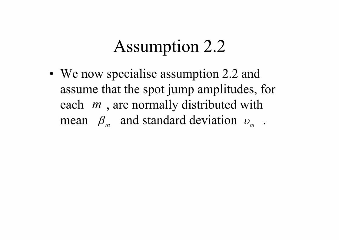
• We now specialise assumption 2.2 and
assume that the spot jump amplitudes, for
each , are normally distributed with
mean and standard deviation .mβ mυ
m

Assumption 2.1
• Assumption 2.1 is unchanged. We write the
known constant spot jump amplitude as mβ

Pricing of standard options
• We would like to price standard (plain
vanilla) European options in a
computationally efficient manner
• (Might allow us to get implied parameters
from market prices of options).
• However, futures commodity prices are
NOT log-normally distributed.
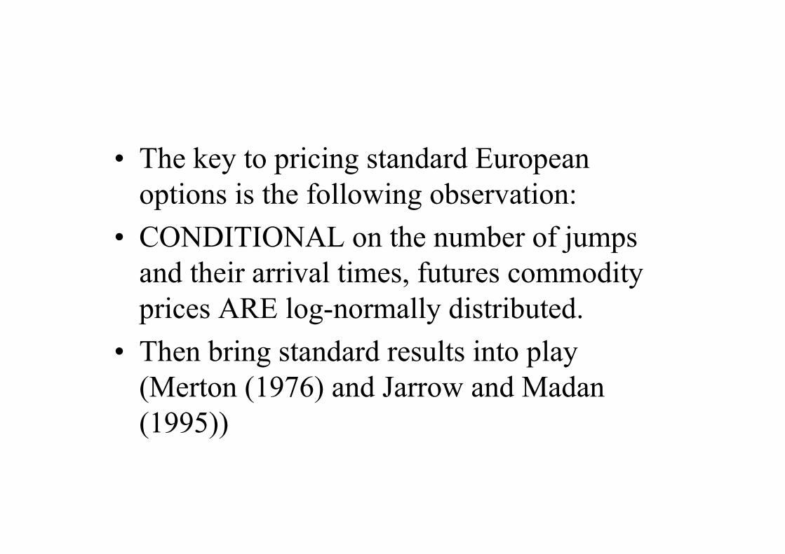
• The key to pricing standard European
options is the following observation:
• CONDITIONAL on the number of jumps
and their arrival times, futures commodity
prices ARE log-normally distributed.
• Then bring standard results into play
(Merton (1976) and Jarrow and Madan
(1995))
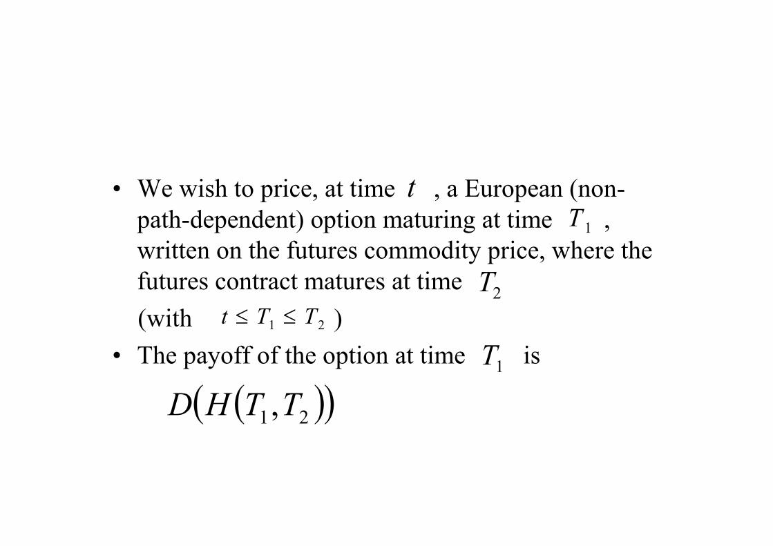
• We wish to price, at time , a European (non-
path-dependent) option maturing at time ,
written on the futures commodity price, where the
futures contract matures at time
(with )
• The payoff of the option at time is
t
1T
2T
21 TTt ≤≤
1T
( )( )21,TTHD
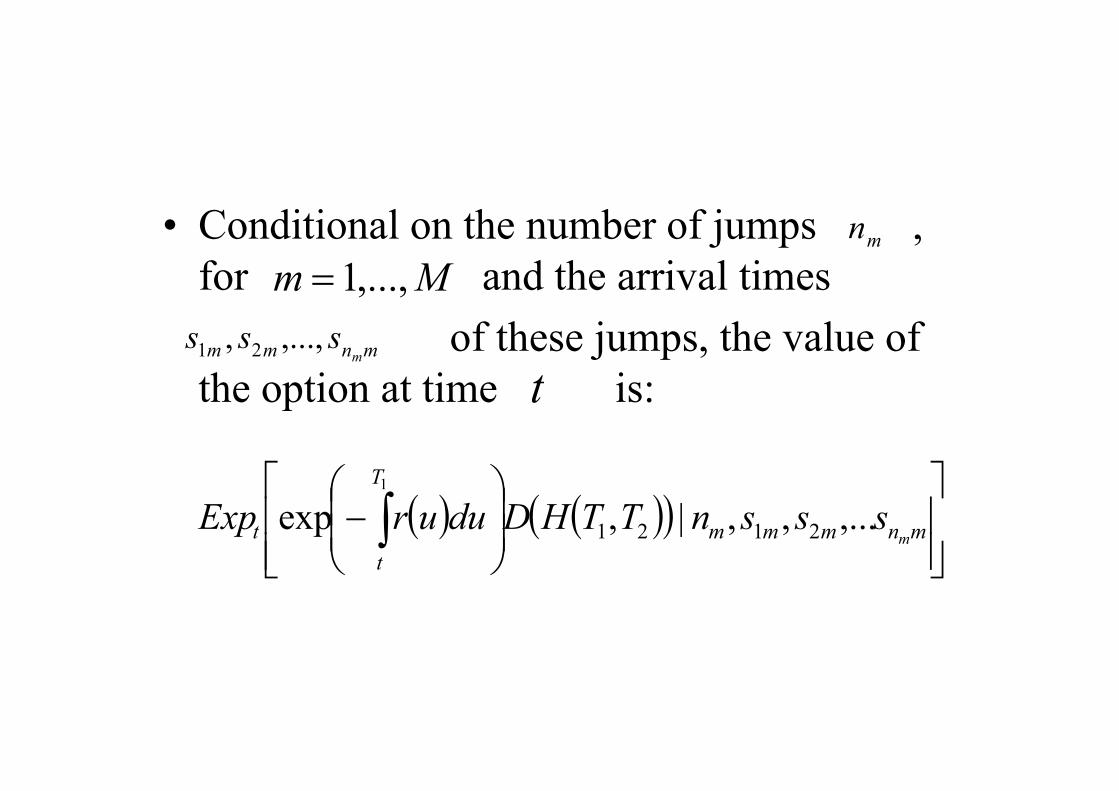
• Conditional on the number of jumps ,
for and the arrival times
of these jumps, the value of
the option at time is:
mn
Mm ,...,1=
mnmm msss ,...,, 21
t
( ) ( )( )
− ∫ mnmmm
T
t
t msssnTTHDduurExp ,...,,|,exp 2121
1

• So using standard results about conditional
expectations and the results earlier:

• The price of the option at time is: t
( ) ( ) ( )∑ ∑ ∑∞=
=
∞=
=
∞=
=
1
1
2
20 0 0
1212111 ;,...;,;,n
n
n
n
n
n
MM
M
M
nTtQnTtQnTtQ
( ) ( )( )∫ ∫ ∫ ∫
−
1 1 1 1
,...,,|,exp... 2121
T
t
T
t
T
t
mnmmm
T
t
t msssnTTHDduurExp
( )[ ] ( )[ ] ( )[ ]
( )Mnn
M
mn
t
t
m
mnmmmmm
Mm
m dsdsdsds
duu
sss......
...12111
1
21
1
0
∏∫
=
λ
λλλ

Standard European Options on
futures• To obtain the form for the price of a standard European options on futures, whose payoff is
Replace
by:
( )( )( )0,,max 21 KTTH −η
( ) ( )( )
− ∫ mnmmm
T
t
t msssnTTHDduurExp ,...,,|,exp 2121
1

Standard European options on
futures
• (looks like Black (1976) formula)
( )1,TtPη
( ) ( ) ( ) ( ) ( )
−
∫ 2121212
1
,,exp,;;,, dKNdNdsTTsAMTnTtVTtH
T
t
m ηη

• Where
• (note this term is simply because of the
stochastic interest-rates – it is the
instantaneous covariance between bond
prices and futures commodity prices)
( ) ( ) ( ) ( ) ( )21
1
2121 ,,,,,, TsTsTsTsTTsA PP
K
k
HkPPHk σσσσρ −
≡ ∑
=

• And (this term depends on number of jumps and
their arrival times)
( )≡MTnTtV m ,;;, 21
( ) ( ) ( )
++
−∑ ∫∑
= =
M
m
mmmm
T
s
m
n
i
mm nduub
im
m
1
2
2.2
1
1.22
11exp1exp
2
υββ
( )
−∑ ∫
=
M
m
T
t
m dsTse1
2
1
,exp

Options continued
• Also we can semi-analytically value:
• Futures-style options (both European and
American) on futures contracts.
• Note that many exchange traded options are
of this type and exchange traded options are
often the most liquid and have the smallest
bid-offer spreads.

Options continued
• We can also semi-analytically value:
• Standard European options on forwards.
• Standard European options on the spot.

Options continued
( ) ( ) ( )∑ ∑ ∑∞=
=
∞=
=
∞=
=
1
1
2
20 0 0
1212111 ;,...;,;,n
n
n
n
n
n
MM
M
M
nTtQnTtQnTtQ
( ) ( )( )∫ ∫ ∫ ∫
−
1 1 1 1
,...,,|,exp... 2121
T
t
T
t
T
t
mnmmm
T
t
t msssnTTHDduurExp
( )[ ] ( )[ ] ( )[ ]
( )Mnn
M
mn
t
t
m
mnmmmmm
Mm
m dsdsdsds
duu
sss......
...12111
1
21
1
0
∏∫
=
λ
λλλ
• Lets look at this formula in more depth.
• Poisson mass functions rapidly tend to zero
once the number of jumps >= mean number
of jumps (=> can truncate infinite sum).
• Need to integrate over arrival times. How?
• Lets look at this formula in more depth.
• Poisson mass functions rapidly tend to zero
once the number of jumps >= mean number
of jumps
• Need to integrate over arrival times. How?
• Monte Carlo - We call this the MCIATJ
methodology in the paper.
• Use Monte Carlo to simulate the arrival
times of the jumps, conditional on the
number of jumps.
• In the special case that the intensity rates
are constants (particularly straightforward),
then the arrival times are uniform on
• (if NOT use inverse transformation
method).
[ ]1,Tt
• It sounds computationally intensive but it
isn’t.
• In the paper, we price 30 options of 5
different strikes and 6 different maturities
• We use anti-thetic variates.
• We use a Control Variate (see paper for
details).
• The options are all standard European calls
on futures prices.
• We demonstrate in the paper that it is
possible to price all 30 options in < 0.51
seconds
• This is < 0.017 seconds per option
• All standard errors < 0.003 % of spot
(mostly even less than 0.001 % of spot).
• MCIATJ is fast for short-dated options.
Calibration
• This means we can obtain the model
parameters from the market prices of
options by doing a least-square fit.
• MCIATJ relatively slow for long-dated
options.
• Is there an even faster way of pricing
standard European options?

Fourier Transforms
• Many authors have shown that it is possible
to price standard European options easily if
the characteristic function of the terminal
asset price is known analytically.
• Carr and Madan (1999), Heston (1993), Lee
(2004), Sepp (2003), Duffie et al. (2000)
• Characteristic function is Fourier Transform
of the probability density function.
Problem
• In our model, the characteristic function is not
analytic if any of the Poisson processes satisfy
Assumption 2.1 with (can be expressed
as an integral but it involves sines and cosines =>
tricky double (oscillatory) integral).
( ) 0>tbm
FTPS methodology
• However, we show that it is possible to
derive a rapidly convergent power series
expansion for terms in the characteristic
function which converges to (say) 10-11
accuracy (or better) after typically about 10
to 40 terms in the series.
• Therefore, very fast, accurate and easy on a
computer.
• We call this the FTPS methodology.

• Multiply FT of payoff by characteristic
function. A single one-dimensional integral
(using eg Simpson’s rule) then gives the
option price.
• This is true even with multiple Brownian
motions and multiple Poisson processes.
With FTPS (Fourier Transform)
methodology:
• Can price the same 30 options in < 0.016 seconds (MCIATJ was 0.51 seconds)
• => less than 1 millisecond per option.
• Can trade time against accuracy.
• But our FTPS (Fourier Transform) methodology is at least 10 times (usually even better) more accurate than the Monte Carlo integration over the arrival times of the jumps (MCIATJ methodology).
Summary
• The model is arbitrage-free.
• Automatically fits initial futures (or
forward) commodity price curve.
• Spot price exhibits mean reversion.
• Long-dated futures can jump less than
short-dated futures.
• Generates stochastic convenience yields
without further ado.
Summary cont’d
• Can price exotics via Monte Carlo.
• Can price standard European options via:
• A Monte Carlo based (MCIATJ) algorithm
or Fourier Transform based (FTPS)
algorithm.
• FTPS is faster and more accurate.

Suggestions for further research 1
• Asian commodity options (also called
commodity swaptions) – approximate
Characteristic Function ??.
• Examine whether or not arbitrage is
possible in case of exponentially dampened
jumps AND random jump amplitudes.

Suggestions for further research 2
• American Options? PDE based approach?
Fourier Transform approach?
• Spread options? See Dempster and Hong
(2000) Judge Institute of Management
Working paper WP26/2000 (published in:
Proceedings of the First World Congress of
the Bachelier Finance Society, Paris
(2000)).