A MOS-based dynamic memetic differential evolution ...jmpena/docs/2011SC.pdf · The fast adaptive memetic algorithm (FAMA) (Caponio et al. 2007), proposed by Caponio et al., is a

FOCUS

A MOS-based dynamic memetic differential evolution algorithmfor continuous optimization: a scalability test

Antonio LaTorre • Santiago Muelas •

Jose-Marıa Pena

Published online: 11 September 2010

� Springer-Verlag 2010

Abstract Continuous optimization is one of the areas

with more activity in the field of heuristic optimization.

Many algorithms have been proposed and compared on

several benchmarks of functions, with different perfor-

mance depending on the problems. For this reason, the

combination of different search strategies seems desirable

to obtain the best performance of each of these approaches.

This contribution explores the use of a hybrid memetic

algorithm based on the multiple offspring framework. The

proposed algorithm combines the explorative/exploitative

strength of two heuristic search methods that separately

obtain very competitive results. This algorithm has been

tested with the benchmark problems and conditions defined

for the special issue of the Soft Computing Journal on

Scalability of Evolutionary Algorithms and other Meta-

heuristics for Large Scale Continuous Optimization Prob-

lems. The proposed algorithm obtained the best results

compared with both its composing algorithms and a set of

reference algorithms that were proposed for the special

issue.

Keywords Continuous optimization � Multiple offspring

sampling � Scalability

1 Introduction

Continuous optimization is a field of research which is

getting more and more attention in the past years. Many

real-world problems from very different domains (biology,

engineering, data mining, etc.) can be formulated as the

optimization of a continuous function. These problems

have been tackled using evolutionary algorithms (EA)

(Muelas et al. 2009) or similar metaheuristics (Tseng and

Chen 2008).

Selecting an appropriate algorithm to solve a continuous

optimization problem is not a trivial task. Although a

particular algorithm can be configured to perform properly

in a given scale of problems (considering the number of

variables as their dimensionality), the behavior of the

algorithm can degrade as this dimensionality increases,

even if the nature of the problem remains the same.

In this contribution, the multiple offspring sampling

(MOS) framework has been used to combine a differential

evolution (DE) algorithm and the first one of the local

searches of the MTS algorithm (through the rest of this

paper we will refer to this local search as MTS-LS1, and its

pseudocode as well as an explanation of how it works can

be found in Tseng and Chen (2008)). This framework

allows the combination of different metaheuristics fol-

lowing a high-level relay hyrbid (HRH) approach (this

nomenclature will be reviewed in Sect. 2) in which the

number of evaluations that each algorithm can carry out is

dynamically adjusted. It will be shown that a MOS-based

algorithm actually obtains the best results compared with

its composing algorithms and a set of reference algorithms

that were proposed for the special issue: DE, Real-Coded

CHC and G-CMA-ES, the best algorithm of the ‘‘Special

Session on Real-Parameter Optimization’’ held at the CEC

2005 Congress. The set of problems that were used for the

A. LaTorre (&) � S. Muelas � J.-M. Pena

Department of Computer Systems Architecture and Technology,

Facultad de Informatica, Universidad Politecnica de Madrid,

Madrid, Spain

e-mail: [email protected]

S. Muelas


J.-M. Pena


123

Soft Comput (2011) 15:2187–2199

DOI 10.1007/s00500-010-0646-3

tests is based on the benchmark of the ‘‘Special Session and

Competition on Large Scale Global Optimization’’ held at

the CEC 2008 congress (Tang et al. 2007), and a set of

additional problem functions of different difficulty types.

The experiments were carried out on a wide range of

dimensions in order to evaluate the behavior of the algo-

rithms as the number of variables increases.

The rest of the paper is organized as follows: In Sect. 2,

relevant related work is briefly reviewed. Section 3 details

the proposed algorithm. In Sect. 4 the experimental sce-

nario is described. Section 5 presents and comments on the

results obtained and lists the most relevant facts from this

analysis. Finally, Sect. 6 contains the concluding remarks

obtained from this work.

2 Related work

The HRH terminology was introduced in Talbi (2002), one

of the first attempts to define a complete taxonomy of

hybrid metaheuristics. This taxonomy is a combination of a

hierarchical and a flat classification structured into two

levels. The first level defines a hierarchical classification in

order to reduce the total number of classes, whereas the

second level proposes a flat classification, in which the

classes that define an algorithm may be chosen in an

arbitrary order. From this taxonomy, the following four

basic hybridization strategies can be derived: (a) LRH

(low-level relay hybrid): one metaheuristic is embedded

into a single-solution metaheuristic. (b) HRH (high-level

relay hybrid): two metaheuristics are executed in sequence.

(c) LTH (low-level teamwork hybrid): one metaheuristic is

embedded into a population-based metaheuristic. (d) HTH

(high-level teamwork hybrid): two metaheuristics are exe-

cuted in parallel.

For this work, we have focused on the HRH group, the

one the algorithm proposed in this paper belongs to.

In the past years there has been an intense research in

HRH or memetic models, combining different types of

metaheuristics. In particular, the DE algorithm is one of the

EA that has been recently hybridized using this kind of

strategy. In the following paragraphs some of the most

recent and representative approaches will be reviewed.

Gao and Wang (2007) proposed CSDE1, a memetic DE,

to optimize thirteen 30-dimensional continuous problems.

CSDE1 uses simplex (Nelder–Mead method) to carry out

the local search (LS) using also chaotic systems to create

the initial population. CSDE1 applies the local search only

to the best individual in the population at each generation.

Tirronen et al. (2007) designed a hybrid DE algorithm

that combined the Hooke–Jeeves Algorithm (HJA) and the

stochastic local search (SLS), coordinated by an adaptive

rule that estimates fitness diversity using the ratio between

the standard deviation and the average fitness of the pop-

ulation. This algorithm was compared against a regular DE

and an evolution strategy (ES) on the problem of weighting

coefficients to detect defects in paper production.

The fast adaptive memetic algorithm (FAMA) (Caponio

et al. 2007), proposed by Caponio et al., is a memetic

algorithm with a dynamic parameter setting and two local

searchers adaptively launched, either one by one or

simultaneously, according to the needs of the evolution.

The employed local search methods are the Hooke–Jeeves

and the Nelder–Mead methods. The Hooke–Jeeves method

is executed only on the elite individual, whereas the

Nelder–Mead simplex is carried out on 11 randomly selected

individuals. FAMA includes a self-adaptive criterium

based on a fitness diversity measure and the iteration

number. Mutation probability and other search parameters

depend also on the diversity measure. the FAMA algorithm

was compared against Tirronen’s algorithm and SFMDE

obtaining better results for the problem of permanent

magnet synchronous motors (Caponio et al. 2008).

There have also been some studies that have tried to

use adaptive learning to combine the algorithms. Ong and

Keane (2004), propose two adaptive strategies, one heu-

ristic and one stochastic, to adapt the participation of

several local searches when combined with a genetic

algorithm (GA). In both strategies, there is a learning phase

in which the performance of each local search is stored and

used in later generations in order to select the local search

to apply. Several local searches are combined with a

metaheuristic algorithm using also an adaptive scheme in

Caponio et al. (2009) and Tirronen et al. (2008). The

application of each algorithm is based on a population

diversity measure which varies among the studies. When

applied to the DE algorithm, this strategy prevents the

stagnation problems of the DE by reducing the excessive

difference between the best individual and the rest of the

population. A quite different approach is followed by

LaTorre et al. (2010). In this work, a hybrid algorithm

combines several genetic algorithms in such a way that

their contribution to the overall search is learned through

the use of Reinforcement Learning techniques. Moreover,

the hybridization strategy learned in one execution of the

algorithm is used and refined in further executions.

In the recent years, there have been several sessions that

have focused on continuous optimization. At the CEC 2005

Congress, a ‘‘Special Session on Real-Parameter Optimi-

zation’’ was carried out for analyzing the performance of

several algorithms on a benchmark of 25 continuous func-

tions (Suganthan et al. 2005). In this competition, the

G-CMA-ES algorithm obtained the best results among all

the evaluated techniques. However, the use of a covariance

matrix makes it not appropriate for high-dimensional

functions. Differential evolution showed to be a competitive

2188 A. LaTorre et al.

123

alternative in ten dimensions: SaDE, a self-adaptive DE

(Qin and Suganthan 2005), obtained the third position in

the final function value, and a real-coded DE algorithm

(Ronkkonen et al. 2005) was ranked third in success

performance.

On the other hand, the ‘‘Special Session and Competi-

tion on Large Scale Global Optimization’’, held at the CEC

2008 Congress, focused on seven functions solved in 100,

500, and 1,000 dimensions (Tang et al. 2007). The MTS

algorithm (Tseng and Chen 2008), which combines several

local searches using a small population, was the best

algorithm of the competition.

Considering these two results, an intuitive approach

would be to combine a local search algorithm, in particular

the first one of those proposed by MTS, with a DE algo-

rithm. This hybrid approach could be seen as the equivalent

to the memetic algorithms in classical genetic algorithms.

For this reason, an HRH algorithm combining these two

algorithms was presented by Muelas et al. (2009) at the

Workshop on Evolutionary Algorithms and other Meta-

heuristics for Continuous Optimization Problems—A Sca-

lability Test held at the ISDA 2009 Conference. In this

algorithm, the hybridization with an exploitative local

search helps the DE to avoid the stagnation problem. On

the other hand, the DE allows the local search to find

promising regions with a moderate consumption of fitness

evaluations. This algorithm proved to deal successfully

with problems of different dimensionality and obtained one

of the best results of the workshop.

3 Proposal

In this section, the MOS framework is reviewed (Sect. 3.1)

and the proposed algorithm is presented (Sect. 3.2).

3.1 Multiple offspring sampling in brief

One of the main advantages of metaheuristics, in general,

and EAs, in particular, is their flexibility and adaptability,

which allows its application to a wide range of optimiza-

tion problems in different domains. However, this charac-

teristic that makes EAs suitable for solving even the

hardest optimization problems with a remarkable success,

is, paradoxically, one of the most important matters that

somebody interested in using these algorithms for his

research has to deal with. An appropriate selection of a

single algorithm and its associated parameters for a par-

ticular optimization problem is a difficult issue (Grefens-

tette (1986), states that this task sometimes becomes an

optimization problem itself).

The No Free Lunch Theorem (Wolpert and Macready

1997) holds that ‘‘any two algorithms are equivalent when

their performance is averaged across all possible prob-

lems‘‘. In other words, this means that it is impossible to

define a general strategy that outperforms any other algo-

rithm for every possible problem. This, of course, applies

for EA. Even if an EA has been proved to be successful on

a similar problem, this does not guarantee that this success

will be repeated. A slight variation on the conditions or the

data used in the experimentation could lead to unpredict-

able results, much of the times not as satisfactory as

expected.

Additionally, several authors report that the hybridiza-

tion of different EAs, encodings or operators can signifi-

cantly boost the performance of the hybrid approach

(Caruana and Schaffer 1988; Mladenovic and Hansen

1997; Schnier and Yao 2000; Thierens 2005; Whitacre

et al. 2006; Lin et al. 2007). This opens new alternatives to

improve the performance by the combination of different

evolutionary approaches and means that now, not only

every single alternative should be considered, but also all

the combinations of any of them.

For this reason, we review in this work the MOS

framework for the development of Dynamic Hybrid EAs

(LaTorre et al. 2009). MOS provides the functional for-

malization necessary to design the aforementioned algo-

rithms, as well as the tools to identify and select the best

performing configuration for the problem under study. In

this context, the hybridization of several algorithms can

lead to the following two situations:

• A collaborative synergy emerges among the different

algorithms that improves the performance of the best

one when it is used individually.

• A competitive selection of the best one takes place, in

which a similar performance (often the same) is

obtained with a minimum overhead.

The hybrid algorithms developed with MOS share many

of the characteristics of traditional EAs. However, there are

some differences between both groups of algorithms. In

MOS, a key term is the concept of technique, which is a

mechanism, decoupled from the main algorithm, to gen-

erate new candidate solutions. This means that, within a

MOS-based algorithm, several offspring mechanisms can

be used simultaneously, and it is the main algorithm which

selects among the available optimization techniques the

most appropriate for the particular problem and search

phase. A more concrete definition for these offspring

mechanisms follows:

Definition 1 In MOS, an offspring technique is a mech-

anism to create new individuals in which(a) a particular

evolutionary algorithm model, (b) an appropriate solution

encoding, (c) specific operators (if required), and (d) nec-

essary parameters have been defined.

A MOS-based dynamic memetic differential evolution algorithm 2189

123

Furthermore, the use of multiple offspring mechanisms

simultaneously has to be controlled in some way. The MOS

framework offers two groups of functions to deal with this

issue: quality and participation functions. The first group of

functions evaluate how good a set of new individuals is

from the point of view of a desirable characteristic. The

second group of functions consider a series of quality

values computed by the first group and adjust the number

of new individuals that each offspring technique will be

allowed to generate in the next step of the search. This way,

the algorithm is able to dynamically adjust the participation

of each of the available techniques and exploit the benefits

of each of them at different stages of the search process.

Finally, the MOS framework allows the development of

both HTH and HRH algorithms (according to Talbi’s

nomenclature seen before).

In the case of the HTH algorithms, the main algorithm

manages an overall population which is shared by all the

techniques. At each generation, the participation of each of

the available techniques is adjusted according to the quality

of the solutions created in the previous generation. Each of

these techniques will produce a percentage of the overall

shared population. A pseudocode of this approach is given

in Algorithm 1. In this pseudocode, Pi represents the

overall shared population at generation i; T ðjÞ is technique

j;OðjÞi the offspring subpopulation produced by technique j

at generation i;QðjÞi the quality value associated to each O

ðjÞi

subpopulation, PðjÞi the participation ratio (percentage of

individuals of the overall shared population) that technique

j can produce at generation i and PF and Q the participa-

tion and quality functions, respectively. Original and off-

spring populations are combined by using any of the

existing elitism procedures, from classic to full elitism,

which most of the times offers the best performance in

terms of quality of the solutions.

On the other hand, in the case of the HRH algorithms

the available techniques are used in sequence, one after the

other, each of them reusing the output population of the

previous technique. This approach fits better when there are

non-population-based techniques, such as local searches, as

these techniques are not constrained to produce a per-

centage of the common population. In this case, the search

process is divided into a fixed number of steps that is

established at the beginning of the execution. Each step is

assigned a constant amount of fitness evaluations (FEsi in

Algorithm 2), which are distributed by the participation

function (PF). Each technique can manage its number of

allocated FEs at each step of the algorithm ðFEsðjÞi Þ in its

own particular way. For example, a population-based

technique, such as DE, could execute several iterations of

the algorithm, whereas a local search could decide to spend

all its assigned evaluations in improving just one individ-

ual. The quality of the new individuals of each technique

will be averaged at the end of the whole set of evaluations

of that step, as the division of the search into generations

depends on each of the techniques. A pseudocode of this

approach is given in Algorithm 2.

3.2 Proposed algorithm

In this contribution, an HRH dynamic memetic DE algo-

rithm is proposed. This algorithm combines the explor-

ative/exploitative strength of two heuristic search methods

that separately obtain very competitive results in either

low- or high-dimensional problems. An HRH approach has

been preferred to an HTH one as it is more natural to allow

each technique to use its assigned FEs in its own way

instead of forcing all the techniques to use a population-

based scheme. Additionally, both algorithms work better

when they can execute for a longer time. Making them

compete for a percent of the offspring population of each


123

generation would lead to a situation in which each tech-

nique would hinder the normal behavior of the other one,

resulting in a poor performance of the hybrid algorithm.

For the adjustment of the participation of each technique

in the overall search process, a new quality function (QF)

has been proposed. This QF takes into account two desir-

able characteristics in a search algorithm: the average fit-

ness increment of the newly created individuals after a set

of allocated fitness evaluations and the number of times

that these improvements take place (Eq. 1).

QðjÞi ¼

RðjÞi�1 if 8k; l 2 ½1; n� : RðkÞi�1 [ RðlÞi�1 )CðkÞi�1 [ CðlÞi�1

CðjÞi�1 otherwise

8>><

>>:

QðjÞi � Quality of technique T ðjÞ in step i

RðjÞi � Average fitness increment of T ðjÞ in step i

CðjÞi � Number of fit. Improvements of T ðjÞ in step i

ð1Þ

This quality function uses the average fitness increment as

the effective QF only if there is consensus between both

measures. If this is not the case, the raw number of fitness

improvements is used. The logic behind this function is

that, in some functions, the use of the average fitness

increment QF could be very elitist. In some particular sit-

uations, a technique which is not carrying out an effective

search could introduce, for some reason, a large increment

in the average fitness value of the new individuals. This

could be due, for example, to a recombination of poor

solutions. In such a case, it is easy for a technique to

improve previous solutions. However, it could be more

adequate to carry out small changes to good individuals in

order to find the right ‘‘path‘‘ to the global optimum rather

than carrying out substantial modifications to poor solu-

tions. For this reason, a consensus of both measures is

required in order to apply the more elitist average fitness

increment QF. If this is not the case, the number of fitness

improvements is used to guarantee a softer adjustment of

participation.

The quality values computed by this QF are used by a

dynamic participation function to adjust the number of

fitness evaluations allocated for each technique at each step

(Eq. 2). This PF computes, at each step, a trade-off factor

for each technique, DðjÞi ; that represents the decrease in

participation for the j-th technique at the j-th step, for every

technique except the best performing ones. These tech-

niques will increase their participation by the sum of all

those DðjÞi divided by the number of techniques with the

best quality values.

PFdynðQðjÞi Þ ¼PðjÞi�1 þ g if j 2 best;

PðjÞi�1 � DðjÞi otherwise

8<

:

g ¼P

k 62best DðkÞi

jbestj

best ¼ fl=QðlÞi �Q

ðmÞi 8l;m 2 ½1; n�g

ð2Þ

The aforementioned DðjÞi values are computed as shown in

Eq. 3. These DðjÞi factors are computed from the relative

difference between the quality of the best and the j-th

techniques, n being the number of available techniques. In

this equation, n represents a reduction factor, i.e., the ratio

that is transferred from one technique to the other(s) (0:05

in this experimentation). Finally, a minimum participation

ratio can be established to guarantee that all the techniques

are represented through all the search. This is done to

avoid, if possible, premature convergence to undesired

solutions caused by a technique that obtains all the

participation in the early steps of the search and quickly

converges to poor regions of the solution space, preventing

the other techniques to collaborate at later stages of the

process, in which they could be more beneficial.

DðjÞi ¼ n � QðbestÞi � Q

ðjÞi

QðbestÞi

�PðjÞi�1 8j 2 ½1; n�=j 6¼ best ð3Þ

Additionally, a population reset method has been also

included in order to avoid a particular situation that has

been observed in some functions in which the whole

population converges to a local optimum very close to the

global optimum. In those cases, all the solutions but one

(the best one, as all the solutions are the same) are uni-

formly re-initialized. This way, the algorithm can reach the

global optimum more easily.

To summarize, the HRH Memetic DE works as follows:

All the available techniques are allocated the same number

of FEs at the beginning of the execution. At the end of each

step, the quality of the new solutions created by each

technique is evaluated and, based on this quality, its par-

ticipation ratio is adjusted accordingly. This participation

ratio is used to compute the number of FEs that each

technique will be allowed to use in the next step of the

search. If a minimum participation ratio has been estab-

lished, then the number of FEs can not go below this

threshold. If the whole population converges to the same

solution, it is reset preserving one copy on the best solution

found so far, to allow the algorithm to converge to the

global optimum.


123

4 Experimentation

4.1 Benchmark suite

A total of 19 continuous optimization functions have been

considered for this experimentation. The first six functions

were originally proposed for the ‘‘Special Session and

Competition on Large Scale Global Optimization’’ held at

the CEC 2008 Congress (Tang et al. 2007). The next five

functions were proposed for the Workshop on Evolutionary

Algorithms and other Metaheuristics for Continuous

Optimization Problems—A Scalability Test held at the

ISDA 2009 Conference. Finally, the last seven functions

are non-separable functions built by combining two func-

tions belonging to the set of functions f 1� f 11: All the

functions are completely scalable functions, which makes

possible the scalability test proposed for this special issue.

A detailed description of the selected benchmark can be

found at the web page of the organizers of the special

issue.1

The results reported for this work are the average of 25

independent executions conducted on the computer con-

figuration displayed in Table 1. For each function, five

different numbers of dimensions have been tested: D ¼50;D ¼ 100;D ¼ 200;D ¼ 500 and D ¼ 1; 000 with a

maximum number of fitness evaluations fixed to 5,000*

dimension. In order to allow an easy comparison with the

composing algorithms of the hybrid approach presented in

this work, as well as with the MDE-DC algorithm pre-

sented in Muelas et al. (2009), the average errors for these

three algorithms are also provided. As suggested by the

organizers of this special issue, all the error values below

1e-14 have been rounded to zero for all the algorithms.

4.2 Parameter tuning

The parameters of the DE technique were selected

according to the extensive parameter tuning that was car-

ried out for the HRH algorithm presented in Muelas et al.

(2009). Regarding the MTS-LS1 technique, it was config-

ured as suggested in the original paper (see (Tseng and

Chen 2008) for further details). Both algorithms, when

used independently, use the same configuration. For this

study, both the population size and the number of steps

parameters were tuned in order to improve the performance

of the algorithm. The population size values that were

explored vary from 10 up to 40 individuals with increments

of 5 individuals. For the number of steps parameter, the

limits were from 50 up to 101 steps with increments of 17

steps, which are roughly equivalent to a 2%; 1:5%; 1:2%and 1% of the overall number of available FEs, respec-

tively. Table 2 displays the final values that were selected

for the algorithm.

Finally, in this work the Differential Evolution tech-

nique has been always chosen as the first algorithm to

execute at the beginning of each step. It seemed reasonable

to execute first the DE in order to provide the LS with a set

of already good solutions instead of carrying out the LS on

a random set of solutions (this could be especially impor-

tant at the beginning of the execution of the algorithm).

However, none other policy has been considered: using

always the LS at the beginning of each step, alternating

both algorithms, choosing randomly, etc. In a further

research, several policies will be tested in order to check if

the order in which the algorithms are executed is relevant

for the performance of the hybrid algorithm.

5 Analysis of the results

In this section, the experimental results obtained with the

proposed algorithm are thoroughly analyzed and validated.

In particular, a statistical analysis on the average error is

conducted, comparing the proposed algorithm against (i) its

composing algorithms, (ii) the MDE-DC algorithm, seed of

this work, presented in Muelas et al. (2009), and (iii) the

reference algorithms specified for this special issue. To

continue, the scalability behavior of the proposed algorithm

is analyzed, from the point of view of the evolution of the

achieved accuracy as the complexity (i.e. the number of

dimensions) of the function grows. Furthermore, the

computational running time of the MOS-based hybrid

algorithm is reported and discussed. Finally, an analysis on

how the participation of each algorithm is adjusted and

Table 1 Computer configuration

PC Intel Xeon 8 cores 1.86 Ghz CPU

Operating system Ubuntu Linux 8.04

Prog. language C??

Compiler GNU C?? 4.3.2

Table 2 Configuration of the MOS-based algorithm

Parameter Value

Population size 15

DE CR 0.5

DE F 0.5

DE crossover operator Exponential

DE selection operator Tournament 2

DE model Classic

Minimum participation ratio 5%

Number of steps 84

1 http://sci2s.ugr.es/eamhco/CFP.php.


123

http://sci2s.ugr.es/eamhco/CFP.php

which quality function is being used at each moment is also

provided.

5.1 Statistical analysis

Tables 3, 4, 5, 6, 7 contain the average error, for each

function and dimension, of the MOS-based hybrid algo-

rithm, both composing algorithms used separately (DE and

MTS-LS1) and the MDE-DC hybrid algorithm. The indi-

vidual DE and MTS-LS1 were run with the same config-

uration of the MOS algorithm, presented in Table 2 (for the

parameters that apply in each case), and the MDE-DC

algorithm was executed with the best configuration found

in its own parameter tuning process (see Muelas et al. 2009

for details). At the bottom of each table, the total number of

functions solved by each algorithm to the aforementioned

precision is reported. As can be seen, the new Dynamic

MOS-based algorithm solves the highest number of func-

tions at any dimension. The difference with regards the

other three algorithms increases as the number of dimen-

sions grows.

It is important to highlight the fact that, in 100 dimen-

sions, the average error for f14 is not zero, as it is in all the

other dimensions. This is due to the convergence problem

to a local optimum commented in Sect.,3.2, that still hap-

pens, although with a smaller probability, even if the

population reset mechanism is being used. However, it is

important to state that only 1 of the 25 independent exe-

cutions present this problem. The remaining executions

converge to the global optimum with a precision higher

than 1e-20.

Once the average errors have been presented, a statis-

tical analysis following the guidelines proposed in Garcıa

et al. (2009) can be carried out. This analysis will be

conducted on two groups of algorithms. First, the proposed

algorithm is compared with its composing techniques and

the MDE-DC algorithm, to prove that this dynamic

hybridization approach is better than the sole use of DE and

MTS-LS1 and also than a static combination of these two

algorithms (MDE-DC). And second, the MOS-based

algorithm is compared with the reference algorithms:

G-CMA-ES, CHC and two DE algorithms with exponential

and binomial crossover, respectively. This comparison has

been done in two steps, considering the average errors up to

500 and 1,000 dimensions, respectively. This is due to the

lack of results for the G-CMA-ES algorithm in 1,000

dimensions as a consequence of the extremely large com-

putation time required to complete those executions.

As for the first statistical comparison, Table 8 shows the

average ranking of MOS, MDE-DC, MTS-LS1, and DE on

the whole set of functions and dimensions. We can see that

the MOS algorithm obtains the best average ranking, fol-

lowed by the other hybrid algorithm, MDE-DC. The two

individual algorithms obtained the worst results.

Table 3 Average error on 50-D functions

Function MOS MDE-DC DE MTS-LS1

Sphere 0.00e?00 0.00e?00 1.50e?00 0.00e?00

Schwefel 2.21 4.64e-13 8.89e-11 4.16e?01 8.84e-11

Rosenbrock 9.61e?00 1.24e?01 5.31e?01 1.63e?02

Rastrigin 0.00e?00 2.38e-01 1.58e?00 0.00e?00

Griewank 0.00e?00 0.00e?00 9.52e-02 7.68e-03

Ackley 0.00e?00 0.00e?00 4.18e-01 0.00e?00

Schwefel 2.22 0.00e?00 0.00e?00 0.00e?00 0.00e?00

Schwefel 1.2 1.54e-08 3.67e-01 1.98e?01 9.56e-12

Extended f10 0.00e?00 0.00e?00 2.07e-03 1.03e?02

Bohachevsky 0.00e?00 0.00e?00 0.00e?00 0.00e?00

Schaffer 0.00e?00 0.00e?00 0.00e?00 1.04e?02

f12 0.00e?00 0.00e?00 4.08e?00 1.34e?01

f13 4.55e-01 6.71e-01 2.82e?01 2.94e?01

f14 0.00e?00 1.98e-01 1.24e?00 5.52e?01

f15 0.00e?00 0.00e?00 0.00e?00 0.00e?00

f16 0.00e?00 0.00e?00 4.38e-01 4.06e?01

f17 1.40e?01 6.12e?00 7.59e?00 2.17e?02

f18 0.00e?00 1.19e-01 4.48e-01 5.65e?01

f19 0.00e?00 0.00e?00 8.39e-02 0.00e?00

Solved funcs. 14 11 4 7



Sphere 0.00e?00 0.00e?00 3.79e?00 1.09e-12

Schwefel 2.21 2.94e12 7.13e-09 7.58e?01 4.66e-10

Rosenbrock 2.03e?01 1.38e?01 1.27e?02 2.32e?02

Rastrigin 0.00e?00 1.19e-01 2.85e?00 1.05e-12

Griewank 0.00e?00 0.00e?00 3.05e-01 6.70e-03

Ackley 0.00e?00 0.00e?00 4.34e-01 1.20e-12

Schwefel 2.22 0.00e?00 0.00e?00 0.00e?00 0.00e?00

Schwefel 1.2 9.17e-02 1.13e?01 4.74e?02 1.43e-03

Extended f10 0.00e?00 0.00e?00 3.71e-03 2.20e?02

Bohachevsky 0.00e?00 0.00e?00 0.00e?00 0.00e?00

Schaffer 0.00e?00 0.00e?00 8.58e-04 2.10e?02

f12 0.00e?00 0.00e?00 2.71e?00 3.91e?01

f13 1.75e?01 2.16e?00 5.87e?01 1.75e?02

f14 1.68e-11 4.46e-01 2.21e?00 2.04e?02

f15 0.00e?00 0.00e?00 0.00e?00 0.00e?00

f16 0.00e?00 0.00e?00 3.52e?00 1.04e?02

f17 1.43e?01 8.51e?00 1.58e?01 4.17e?02

f18 0.00e?00 3.97e-01 8.76e-01 1.22e?02

f19 0.00e?00 0.00e?00 0.00e?00 0.00e?00



123

In order to provide a proper statistical validation of the

results, Holm’s, Hochberg’s and Wilcoxon procedures

have been used. In the case of the Wilcoxon test, the

adjusted p value is computed as described in Garcıa et al.

(2009), to allow the comparison of multiple algorithms

avoiding the Family-Wise Error (FWER) that multiple

pair-wise comparisons could have introduced. The results

of these tests are reported in Table 11, and show, for all of

them, that there is statistical evidence to state that the MOS

algorithm is better than any of the algorithms considered in

the comparison.

Tables 9 and 10 present the average ranking of the

comparison of MOS with the reference algorithms up to

500 and 1,000 dimensions, respectively. As it was

remarked before, two different comparisons have been

needed due to the lack of results for the G-CMA-ES

algorithm in 1,000 dimensions (Table 11).

In both tables we can see that the best average ranking is

obtained by the MOS-based algorithm, followed by the two

DE algorithms, the G-CMA-ES algorithm and the worst

results are for the CHC algorithm. The differences are

especially important with the DE with binomial crossover,

the G-CMA-ES and the CHC algorithms.

With these results in mind, the same statistical valida-

tion described in the previous paragraphs has been

employed. Tables 12 and 13 present the results of this

statistical validation up to 500 and 1,000 dimensions,

respectively, which concludes that the algorithm presented

in this work is statistically better than any of the reference

algorithms considering any of the validation procedures.



Sphere 0.00e?00 0.00e?00 8.55e?00 2.29e-12

Schwefel 2.21 1.24e-11 3.75e-09 1.05e?02 4.54e-09

Rosenbrock 4.01e?01 2.29e?01 3.32e?05 1.69e?02

Rastrigin 0.00e?00 1.19e-01 6.98e?00 2.34e-12

Griewank 0.00e?00 0.00e?00 4.05e-01 5.42e-03

Ackley 0.00e?00 0.00e?00 7.14e-01 2.38e-12

Schwefel 2.22 0.00e?00 0.00e?00 0.00e?00 0.00e?00

Schwefel 1.2 1.16e?02 2.91e?02 5.76e?03 1.42e?01

Extended f10 0.00e?00 4.03e-07 8.79e-03 4.27e?02

Bohachevsky 0.00e?00 0.00e?00 4.19e-02 0.00e?00

Schaffer 0.00e?00 5.15e-07 5.07e-03 4.28e?02

f12 0.00e?00 3.09e-11 3.61e?00 8.42e?01

f13 9.03e?00 1.66e?01 1.49e?02 2.53e?02

f14 0.00e?00 9.24e-01 4.75e?00 3.89e?02

f15 0.00e?00 0.00e?00 0.00e?00 0.00e?00

f16 0.00e?00 9.23e-10 3.70e?00 1.97e?02

f17 5.03e?00 1.35e?01 2.23e?01 6.07e?02

f18 0.00e?00 2.78e-01 2.37e?00 2.34e?02

f19 0.00e?00 0.00e?00 4.19e-02 0.00e?00




Sphere 0.00e?00 0.00e?00 2.46e?01 5.77e-12

Schwefel 2.21 5.51e-04 3.80e-04 1.44e?02 5.34e-06

Rosenbrock 4.57e?01 2.57e?01 1.12e?05 2.20e?02

Rastrigin 0.00e?00 1.02e-12 1.63e?01 5.62e-12

Griewank 0.00e?00 0.00e?00 4.73e-01 4.24e-03

Ackley 0.00e?00 0.00e?00 1.06e?00 6.18e-12

Schwefel 2.22 0.00e?00 0.00e?00 0.00e?00 1.46e-12

Schwefel 1.2 1.28e?04 1.09e?04 6.70e?04 6.16e?03

Extended f10 0.00e?00 3.41e?00 1.12e-02 1.00e?03


Schaffer 0.00e?00 3.36e?00 2.43e-01 1.00e?03

f12 0.00e?00 4.08e-01 1.16e?01 2.47e?02

f13 3.78e?01 4.84e?01 4.02e?02 5.05e?02

f14 0.00e?00 1.89e?00 1.16e?01 1.10e?03

f15 0.00e?00 1.39e-11 4.19e-02 1.08e-12

f16 0.00e?00 9.97e-01 1.32e?01 4.99e?02

f17 1.21e?01 2.76e?01 6.94e?01 7.98e?02

f18 0.00e?00 1.05e?00 3.87e?00 5.95e?02

f19 0.00e?00 0.00e?00 8.39e-02 0.00e?00


Table 7 Average error on 1,000-D functions


Sphere 0.00e?00 1.02e-12 3.71e?01 1.15e-11

Schwefel 2.21 4.25e-01 1.02e-01 1.63e?02 2.25e-02

Rosenbrock 6.15e?01 2.45e?01 1.59e?05 2.10e?02

Rastrigin 0.00e?00 2.95e?00 3.47e?01 1.15e-11

Griewank 0.00e?00 0.00e?00 7.36e-01 3.55e-03

Ackley 0.00e?00 3.01e-12 8.70e-01 1.24e-11

Schwefel 2.22 0.00e?00 0.00e?00 0.00e?00 0.00e?00

Schwefel 1.2 1.94e?05 1.45e?05 3.15e?05 1.23e?05

Extended f10 0.00e?00 1.32e?02 6.26e-02 1.99e?03


Schaffer 0.00e?00 1.34e?02 4.42e-02 1.99e?03

f12 0.00e?00 3.24e?01 2.58e?01 5.02e?02

f13 8.80e?01 2.41e?02 8.24e?04 8.87e?02

f14 0.00e?00 1.96e?01 2.39e?01 2.23e?03

f15 0.00e?00 0.00e?00 2.11e-01 0.00e?00

f16 0.00e?00 6.70e?01 1.83e?01 1.00e?03

f17 2.25e?01 2.19e?02 1.76e?05 1.56e?03

f18 0.00e?00 3.26e?01 7.55e?00 1.21e?03

f19 0.00e?00 0.00e?00 2.51e-01 0.00e?00



123

5.2 Scalability analysis

In this section we analyze the scalability behavior of the

proposed algorithm. In general, the MOS algorithm

exhibits an excellent scalability behavior. In Tables 3, 4,

5, 6, 7 it can be seen that our algorithm solves the same

number of functions, 14, regardless their dimensionality

(except in 100 dimensions, in which f14 does not converge

in 1 out of the 25 independent executions, as it was men-

tioned before). On the other hand, the other algorithms

under study see how their performance degrades as the

number of dimensions increases. For the five remaining

functions, which are not solved at any dimension, the

behavior of the proposed algorithm is different. The order

of magnitude of the average error of the first group of

functions, made up of Rosenbrock, f13 and f17 functions,

grows linearly, although it is almost constant, with the

number of dimensions (see Fig. 1). Both hybrid functions,

f13 ad f17, have in common that they are combinations of

Rosenbrock’s function with another function, so it is nor-

mal that their scalability behavior is linked to that exhibited

by the individual function. In this function, there is a very

narrow valley that goes from local optimum to global

optimum. Finding that valley is difficult and, for that rea-

son, there is a high deviation in the average errors of dif-

ferent executions. However, reaching average regions of

the solutions space should be relatively easy for a good

search algorithm, which explains why the average errors

remain more or less constant (or at least in similar orders of

magnitude) regardless of the number of dimensions.

Regarding the other two functions, the order of magni-

tude of the average error for Schwefel’s 1.2 seems to grow

more or less logarithmically with the number of dimen-

sions, whereas for Schwefel’s problem 2.21 it is not clear at

all. Both functions are unimodal and not separable nor

easily optimized dimension by dimension. However,

Bohachevsky’s function shares the same characteristics

(and Griewank’s, except for the unimodality) and they can

be solved by the MOS algorithm, so the difficulty issue

should be at a different place.

If we pay more attention to Schwefel’s problem 2.21, we

can see that it presents large neutral areas, as the final

fitness of solution is only determined by the value of one

single dimension (the one with the highest absolute value).

The effect of this characteristic is more pronounced as

the number of dimensions is increased. Furthermore, the

dimension with more influence in the final fitness value can

change from one solution to another or when a solution is

modified, so this information can not be exploited by the

search algorithm, which makes more difficult to find an

optimal solution. Both characteristics could explain the

scalability behavior of the proposed algorithm on this

function.

Considering now Schwefel’s problem 1.2, we can see

that, in this case, the influence of some components (the

first ones, in particular) on the final fitness value is even

more pronounced in this function than in the previous one.

This probably explains why the average error quickly

increases as the dimensionality of the problem grows,

especially for the first numbers of dimensions that have

been tested. When the number of dimensions increases up

to 500–1,000, the average errors are so large that the

influence of this characteristic is not as important as in

smaller dimensions.

5.3 Running time analysis

In the previous section we conducted a scalability analysis

from the point of view of the average error. In this section,

a similar analysis is carried out on the computational run-

ning time. For each function and dimension, the running

time of the algorithm at each execution has been recorded

and averaged. Tables 14 and 15 show this information,

which is expressed in seconds.

Table 8 Average ranking for the first comparison up to 1,000

dimensions

Ranking

MOS 1.56

MDE-DC 2.09

MTS-LS1 3.05

DE 3.31

Table 9 Average ranking for the second comparison up to 500

dimensions

Ranking

MOS 1.36

DEExp 2.18

DEBin 3.43

G-CMA-ES 3.70

CHC 4.32

Table 10 Average ranking for the second comparison up to 1,000

dimensions

Ranking

MOS 1.22

DEExp 1.94

DEBin 3.18

CHC 3.66


123

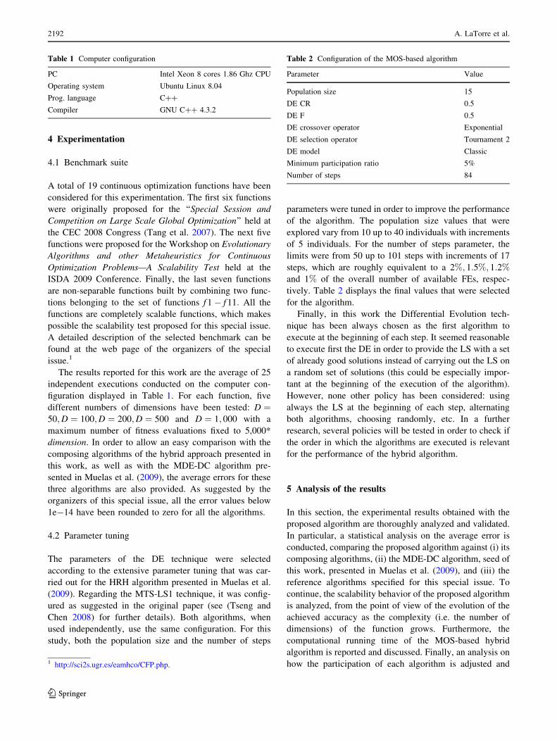
Figure 2 plots the information gathered in Tables 14 and

15. In this figure, the computational running time as the

number of dimensions grows has been represented for all

the functions. It can be seen that the required computa-

tional time seems to grow quadratically with the number of

dimensions of the function. Using the Big Theta notation,

we could say that the computational time of the MOS

algorithm ðf ðnÞÞ is Hðn2Þ; being k1 and k2 two constants

such as the following expression is satisfied:

k1 � n2 � f ðnÞ � k1 � n2

The values for these two constants can be roughly be

established to 11400

and 1400; respectively. These values are

relatively large, and they help to soften the effect of the

quadratic function. In conclusion, the running time of the

proposed algorithm seems to scale well up to a large

number of dimensions.

5.4 Participation and quality analysis

We conclude the analysis of the proposed algorithm by

studying its dynamic behavior with regard to the adjust-

ment of the participation of each technique on the overall

search process and the selection of the effective quality

function to be used at each moment.

Regarding the adjustment of the participation of the two

considered techniques, we have observed three different

behaviors:

• Clear dominance of the DE technique. This happens

with Ackley, f12, f14, f16, f18 and Sphere.

• Clear dominance of the MTS-LS1 technique. This is the

case for Schwefel 1.2.

Table 11 Statistical validation for the first comparison (MOS is the control algorithm)

MOS vs. z value p value Holm p value Hochberg p value Wilcox p value

MDE-DC 2.84e?00 4.54e-03 4.54e-03* 4.54e-03* 5.55e-04*

MTS-LS1 7.95e?00 1.78e-15 3.55e-15* 3.55e-15* 8.42e-10*

DE 9.33e?00 0.00e?00 0.00e?00* 0.00e?00* 6.80e-15*

Wilcox p value with FWER: MOS vs. MDE-DC, MTS-LS1, DE 5.55e-04*

* Means that there are statistical differences with significance level a = 0.05

Table 12 Statistical validation for the second comparison up to 500 dimensions (MOS is the control algorithm)


CHC 1.15e?01 0.00e?00 0.00e-00* 0.00e-00* 1.80e-14*

DEExp 3.21e?00 1.35e-03 1.35e-03* 1.35e-03* 5.96e-09*

DEBin 8.05e?00 8.88e-16 1.78e-15* 1.78e-15* 3.54e-13*

G-CMA-ES 9.13e?00 0.00e?00 0.00e?00* 0.00e?00* 7.764e-11*

Wilcox p value with FWER: MOS vs. CHC, DEExp, DEBin, G-CMA-ES 6.04e-09*


Table 13 Statistical validation for the second comparison up to 1,000 dimensions (MOS is the control algorithm)


CHC 1.30e?01 0.00e?00 0.00e?00* 0.00e?00* 1.30e-1.7*

DEExp 3.85e?00 1.18E-04 1.18e-04* 1.18e-04* 3.87e-11*

DEBin 1.05e?01 0.00e?00 0.00e?00* 0.00e?00* 2.35e-16*

Wilcox p value with FWER: MOS vs. CHC, DEExp, DEBin 3.87e-11*


Fig. 1 Scalability plots for MOS in logarithmic scale


123

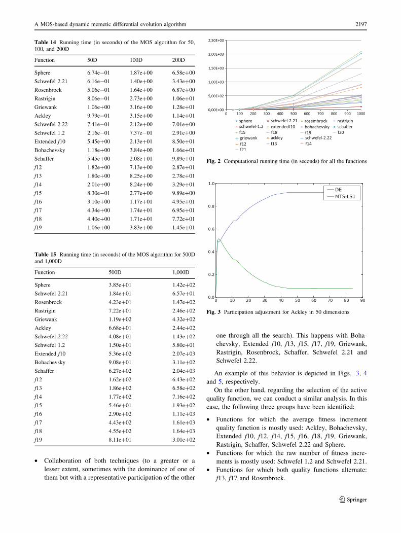
• Collaboration of both techniques (to a greater or a

lesser extent, sometimes with the dominance of one of

them but with a representative participation of the other

one through all the search). This happens with Boha-

chevsky, Extended f10, f13, f15, f17, f19, Griewank,

Rastrigin, Rosenbrock, Schaffer, Schwefel 2.21 and

Schwefel 2.22.

An example of this behavior is depicted in Figs. 3, 4

and 5, respectively.

On the other hand, regarding the selection of the active

quality function, we can conduct a similar analysis. In this

case, the following three groups have been identified:

• Functions for which the average fitness increment

quality function is mostly used: Ackley, Bohachevsky,

Extended f10, f12, f14, f15, f16, f18, f19, Griewank,

Rastrigin, Schaffer, Schwefel 2.22 and Sphere.

• Functions for which the raw number of fitness incre-

ments is mostly used: Schwefel 1.2 and Schwefel 2.21.

• Functions for which both quality functions alternate:

f13, f17 and Rosenbrock.

Table 14 Running time (in seconds) of the MOS algorithm for 50,

100, and 200D

Function 50D 100D 200D

Sphere 6.74e-01 1.87e?00 6.58e?00

Schwefel 2.21 6.16e-01 1.40e?00 3.43e?00

Rosenbrock 5.06e-01 1.64e?00 6.87e?00

Rastrigin 8.06e-01 2.73e?00 1.06e?01

Griewank 1.06e?00 3.16e?00 1.28e?01

Ackley 9.79e-01 3.15e?00 1.14e?01

Schwefel 2.22 7.41e-01 2.12e?00 7.01e?00

Schwefel 1.2 2.16e-01 7.37e-01 2.91e?00

Extended f10 5.45e?00 2.13e?01 8.50e?01

Bohachevsky 1.18e?00 3.84e?00 1.66e?01

Schaffer 5.45e?00 2.08e?01 9.89e?01

f12 1.82e?00 7.13e?00 2.87e?01

f13 1.80e?00 8.25e?00 2.78e?01

f14 2.01e?00 8.24e?00 3.29e?01

f15 8.30e-01 2.77e?00 9.89e?00

f16 3.10e?00 1.17e?01 4.95e?01

f17 4.34e?00 1.74e?01 6.95e?01

f18 4.40e?00 1.71e?01 7.72e?01

f19 1.06e?00 3.83e?00 1.45e?01

Table 15 Running time (in seconds) of the MOS algorithm for 500D

and 1,000D

Function 500D 1,000D

Sphere 3.85e?01 1.42e?02

Schwefel 2.21 1.84e?01 6.57e?01

Rosenbrock 4.23e?01 1.47e?02

Rastrigin 7.22e?01 2.46e?02

Griewank 1.19e?02 4.32e?02

Ackley 6.68e?01 2.44e?02

Schwefel 2.22 4.08e?01 1.43e?02

Schwefel 1.2 1.50e?01 5.80e?01

Extended f10 5.36e?02 2.07e?03

Bohachevsky 9.08e?01 3.11e?02

Schaffer 6.27e?02 2.04e?03

f12 1.62e?02 6.43e?02

f13 1.86e?02 6.58e?02

f14 1.77e?02 7.16e?02

f15 5.46e?01 1.93e?02

f16 2.90e?02 1.11e?03

f17 4.43e?02 1.61e?03

f18 4.55e?02 1.64e?03

f19 8.11e?01 3.01e?02

Fig. 2 Computational running time (in seconds) for all the functions

Fig. 3 Participation adjustment for Ackley in 50 dimensions


123

It can be seen that, for most of the functions, the average

fitness increment is preferred to guide the adjustment of the

participation of the techniques. However, there are some

specific functions for which it is important to conduct small

changes on the solutions rather than large modifications

with important fitness increments.

The active quality function for one function of each

group is depicted in Figs. 6, 7 and 8, respectively.

6 Conclusions

In this work, a new hybrid memetic algorithm based on the

MOS framework has been presented and thoroughly tested

on a large set of scalable continuous functions. Different

numbers of dimensions have been tested to study the sca-

lability behavior of the algorithm. The hybrid algorithm

has been statistically compared with each of its composing

algorithms, as well as with a static combination of both

algorithms. All the considered statistical tests found

Fig. 4 Participation adjustment for Schwefel 1.2 in 50 dimensions

Fig. 5 Participation adjustment for f17 in 50 dimensions

Fig. 6 Active quality function for Ackley in 1,000 dimensions

Fig. 7 Active quality function for Schwefel 1.2 in 1,000 dimensions

Fig. 8 Active quality function for Rosenbrock in 1,000 dimensions


123

significant differences, which means that the MOS-based

algorithm outperforms all the other algorithms. The same

validation procedure has been conducted to compare our

approach with several reference algorithms, classic in the

literature of continuous optimization (CHC, two DEs and

G-CMA-ES). Once again, the statistical tests found sig-

nificant differences between the MOS-based algorithm and

all the other algorithms. This allows us to state that the

algorithm presented in this work is better than any of these

reference approaches for this benchmark.

Regarding the scalability issue, the proposed algorithm

has been able to keep a stable behavior regardless the

dimensionality of the problem. 14 out of the 19 functions

of the benchmark have been solved to the maximum pos-

sible precision in all the considered dimensions. For the

remaining functions, the order of magnitude of the average

error grows differently, with only one function with a rel-

atively bad scalability behavior.

Finally, the computational running time has also been

examined. The results show that the required computa-

tional time grows more or less quadratically. However, this

time is scaled by a factor that reduces the actual compu-

tational time to reasonable values up to relatively large

numbers of dimensions.

Acknowledgments This work was supported by the Madrid

Regional Education Ministry and the European Social Fund, financed

by the Spanish Ministry of Science TIN2007-67148 and supported by

the Cajal Blue Brain Project. The authors thankfully acknowledge the

computer resources, technical expertise and assistance provided

by the Centro de Supercomputacion y Visualizacion de Madrid

(CeSViMa) and the Spanish Supercomputing Network.

References

Caponio A, Cascella G, Neri F, Salvatore N, Sumner M (2007) A fast

adaptive memetic algorithm for on-line and off-line control

design of PMSM drives. IEEE Trans Syst Man Cybern Part B

37:28–41

Caponio A, Neri F, Cascella G, Salvatore N (2008) Application of

memetic differential evolution frameworks to PMSM drive

design. In: Proceedings of the 2008 IEEE congress on evolu-

tionary computation, CEC 2008 (IEEE World Congress on

Computational Intelligence), pp 2113–2120

Caponio A, Neri F, Tirronen V (2009) Super-fit control adaptation in

memetic differential evolution frameworks. Soft Comput Fusion

Found Methodol Appl 13(8):811–831

Caruana R, Schaffer J (1988) Representation and hidden bias: Gray

vs. binary coding for genetic algorithms. In: Proceedings of the

5th international conference on machine learning, ICML 1998,

pp 153–161

Gao Y, Wang Y-J (2007) A memetic differential evolutionary

algorithm for high dimensional functions’ optimization. In:

Proceedings of the third international conference on natural

computation (ICNC 2007), pp 188–192

Garcıa S, Molina D, Lozano M, Herrera F (2009) A study on the use

of non-parametric tests for analyzing the evolutionary algorithms

behaviour: a case study on the CEC2005 special session on real

parameter optimization. J Heurisics 15(6):617–644

Grefenstette J (1986) Optimization of control parameters for genetic

algorithms. IEEE Trans Syst Man Cybern 16(1):122–128

LaTorre A (2009) A framework for hybrid dynamic evolutionary

algorithms: multiple offspring sampling (mos). Ph.D. thesis,

Universidad Politecnica de Madrid (November 2009)

LaTorre A, Pena J, Muelas S, Freitas A (2010) Learning hybridization

strategies in evolutionary algorithms. Intell Data Anal 14(3)

Lin G, Kang L, Chen Y, McKay B, Sarker R (2007) A self-adaptive

mutations with multi-parent crossover evolutionary algorithm for

solving function optimization problems. In: Kang L, Zeng YLS

(eds) Advances in computation and intelligence: proceedings of

the 2nd international symposium, ISICA 2007. Lectures notes in

computer science, vol 4683/2007, pp 157–168

Mladenovic N, Hansen P (1997) Variable neighborhood search.

Comput Oper Res 24(11):1097–1100

Muelas S, LaTorre A, Pena J (2009) A memetic differential evolution

algorithm for continuous optimization. In: Proceedings of the 9th

international conference on intelligent systems design and

applications, ISDA 2009, pp 1080–1084

Ong Y-S, Keane A (2004) Meta-lamarckian learning in memetic

algorithms. IEEE Trans Evol Computat 8(2):99–110

Qin A, Suganthan P (2005) Self-adaptive differential evolution

algorithm for numerical optimization. In: Proceedings of the

IEEE congress on evolutionary computation, CEC 2005,

pp 1785–1791

Ronkkonen J, Kukkonen S, Price K (2005) Real-parameter optimi-

zation with differential evolution. In: Proceedings of the IEEE

congress on evolutionary computation, CEC 2005, pp 506–513

Schnier T, Yao X (2000) Using multiple representations in evolu-

tionary algorithms. In: Proceedings of the 2nd IEEE congress on

evolutionary computation, CEC 2000, vol 1, pp 479–486

Suganthan P, Hansen N, Liang J, Deb K, Chen Y, Auger A, Tiwari S

(2005) Problem definitions and evaluation criteria for the cec

2005 special session on real-parameter optimization. Tech. Rep.

2005005, 1School of EEE. Nanyang Technological University

and Kanpur Genetic Algorithms Laboratory (KanGAL)

Talbi E-G (2002) A taxonomy of hybrid metaheuristics. J Heuristics

8(5):541–564

Tang K, Yao X, Suganthan P, MacNish C, Chen Y, Chen C, Yang Z

(2007) Benchmark functions for the cec 2008 special session and

competition on large scale global optimization. Tech. rep., Nature

Inspired Computation and Applications Laboratory, USTC

Thierens D (2005) An adaptive pursuit strategy for allocating operator

probabilities. In: Proceedings of the 7th genetic and evolutionary

computation conference, GECCO 2005, pp 1539–1546

Tirronen V, Neri F, Karkkainen T, Majava K, Rossi T (2007) A

memetic differential evolution in filter design for defect

detection in paper production. In: Proceedings of EvoWorkshops

2007, pp 330–339

Tirronen V, Neri F, Karkkainen T, Majava K, Rossi T (2008) An

enhanced memetic differential evolution in filter design for defect

detection in paper production. Evol Comput 16(4):529–555

Tseng L, Chen C (2008) Multiple trajectory search for large scale

global optimization. In: Proceedings of the 10th IEEE congress

on evolutionary computation, CEC 2008 (IEEE World Congress

on Computational Intelligence). IEEE Press, pp 3052–3059

Whitacre J, Pham T, Sarker R (2006) Credit assignment in adaptive

evolutionary algorithms. In: Proceedings of the 8th genetic and

evolutionary computation conference, GECCO 2006, Seattle,

pp 1353–1360

Wolpert D, Macready W (1997) No free lunch theorems for

optimization. IEEE Trans Evol Comput 1(1):67–82


123

Documents

A MOS-based dynamic memetic differential evolution ...jmpena/docs/2011SC.pdf · The fast adaptive memetic algorithm (FAMA) (Caponio et al. 2007), proposed by Caponio et al., is a