A MOPSO Algorithm Based Exclusively on

Pareto Dominance Concepts

Julio E. Alvarez-Benitez?, Richard M. Everson and Jonathan E. Fieldsend??

Department of Computer Science, University of Exeter, UK

Abstract In extending the Particle Swarm Optimisation methodologyto multi-objective problems it is unclear how global guides for particlesshould be selected. Previous work has relied on metric information inobjective space, although this is at variance with the notion of domi-nance which is used to assess the quality of solutions. Here we proposemethods based exclusively on dominance for selecting guides from a non-dominated archive. The methods are evaluated on standard test problemsand we find that probabilistic selection favouring archival particles thatdominate few particles provides good convergence towards and cover-age of the Pareto front. We demonstrate that the scheme is robust tochanges in objective scaling. We propose and evaluate methods for con-fining particles to the feasible region, and find that allowing particles toexplore regions close to the constraint boundaries is important to ensureconvergence to the Pareto front.

1 Introduction

Evolutionary algorithms (EA) have been used since the mid-eighties to solvecomplex single and multi-objective optimisation problems (see, for example,[1,2,3]). More recently the Particle Swarm Optimisation (PSO) heuristic, in-spired by the flocking and swarm behaviour of birds, insects, and fish schoolshas been successfully used for single objective optimisation, such as neural net-work training and non-linear function optimisation [4]. Briefly, PSO maintainsa balance between exploration and exploitation in a population (swarm) of so-lutions by moving each solution (particle) towards both the global best solutionlocated by the swarm so far and towards the best solution that the particularparticle has so far located. The global best and personal best solutions are oftencalled guides.

Since PSO and EA algorithms have structural similarities (such as the pres-ence of a population searching for optima and information sharing betweenpopulation members) it seems a natural progression to extend PSO to multi-objective problems (MOPSO). Some attempts in this direction have been madewith promising results such as [5,6,7,8,9]. In the most recent heuristics the guidesare selected from the set of non-dominated solutions found so far. However, in

? Supported by and currently with Banco de la Republica, Colombia.?? Supported by EPSRC, grant GR/R24357/01.

a multi-objective problem each of non-dominated solutions is a potential globalguide and there are many ways of selecting a guide from among them for eachparticle in the swarm. Heuristics to date have relied on proximity in objectivespace to determine this selection, however the relative weightings of the objec-tives are a priori unknown and the use of metric information in objective spaceis at variance with the notion of dominance that is central to the definition ofPareto optimality. In this paper we propose and examine MOPSO heuristicsbased entirely on Pareto dominance concepts. The manner in which particlesare constrained to lie within the search space can have a marked effect on theoptimisation efficiency: the other central purpose of this paper is to propose andcompare constraint methods.

We start by briefly reviewing basic definitions of multi-objective problemsand Pareto concepts (section 2), after which we describe the single objectivePSO methodology in section 3. The multi-objective PSO algorithm is presentedin section 4, and we present and evaluate methods for selecting guides here. Tech-niques for confining particles to the feasible region are described and evaluatedin section 5. Finally, conclusions are drawn in section 6.

2 Dominance and Pareto optimality

In a multi-objective optimisation problem we seek to simultaneously extremiseD objectives: yi = fi (x), where i = 1, . . . , D and where each objective dependsupon a vector x of K parameters or decision variables. The parameters may alsobe subject to the J constraints: ej (x) ≥ 0 for j = 1, . . . , J .

Without loss of generality it is assumed that these objectives are to be min-imised, as such the problem can be stated as:

minimise y = f (x) ≡ (f1 (x) , f2 (x) , . . . , fD (x)) (1)

subject to e (x) ≡ (e1(x) , e2 (x) , . . . , eJ (x)) ≥ 0. (2)

A decision vector u is said to strictly dominate another v (denoted u ≺ v) iffi (u) ≤ fi (v) ∀i = 1, . . . , D and fi (u) < fi (v) for some i; less stringently u

weakly dominates v (denoted u � v) if fi(u) ≤ fi(v) for all i. A set of decisionvectors is said to be a non-dominated set if no member of the set is dominatedby any other member. The true Pareto front, P , is the non-dominated set ofsolutions which are not dominated by any feasible solution.

3 Particle Swarm Optimisation – PSO

The particle swarm optimisation method evolved from a simple simulation modelof the movement of social groups such as birds and fish [4], in which it wasobserved that local interactions underlie the group behaviour and individualmembers of the group can profit from the discoveries and experiences of other

2

members. In PSO each solution (particle) xn in the swarm of N particles isendowed with a velocity which determines its location at the next time step:

x(t+1)n = x(t)

n + χv(t)n + ε

(t) (3)

where χ ∈ [0, 1] is a constriction factor which controls the velocity’s magnitude;in the work reported here χ = 1. The final term in (3) is a small stochastic per-turbation, known as the turbulence factor, added to the position to help preventthe particle becoming stuck in local minima and to promote wide exploration ofthe decision space. Although originally introduced as a normal perturbation [8],here a perturbation to each dimension was added with probability 0.01 and εk

itself was a perturbation from a Laplacian density p(εk) ∝ e−|εk|/β with β = 0.1.The Laplacian distribution yields occasional large perturbations thus enablingwider exploration.

The velocities of each particle are modified to fly towards two different guides:their personal best, Pn, for exploiting the best results found so far by each ofthe particles, and the global best, G, the best solution found so far by the wholeswarm for encouraging further exploration and information sharing between theparticles. This is achieved by updating the K components of each particle’svelocity as follows:

v(t+1)nk = wv

(t)nk + c1r1(Pnk − x

(t)nk) + c2r2(Gnk − x

(t)nk) (4)

r1 and r2 are two uniformly distributed random numbers in the range [0, 1]. Theconstants c1 and c2 control the effect of the personal and global guides, and theparameter w, known as the inertia, controls the trade-off between global andlocal experience; large w motivates global exploration by giving large weight tothe current velocity. In the work reported here c1 = c2 = 1 and w = 0.5. Theglobal guide carries a subscript n because for multi-objective PSO a (possiblydifferent) global guide is associated with each particle; this is in contrast to uni-objective PSO in which there is a single global guide, namely the best solutionlocated so far.

4 Multi-objective PSO

The main difficulty in extending PSO to multi-objective problems is to find thebest way of selecting the guides for each particle in the swarm; the difficultyis manifest as there are no clear concepts of personal and global bests thatcan be clearly identified when dealing with D objectives rather than a singleobjective. Previous MOPSO implementations [5,6,7,8,9,10] have all used metricsin objective space (either explicitly or implicitly) in the selection of guides – thusmaking them susceptible to different scalings in objective space.

The algorithms we propose here are similar to recent MOPSO algorithms[7,8,9,10] in that they use an archive or repository, A, which contains the non-dominated solutions found by the algorithm so far. We emphasise that we do not

3

Algorithm 1 Multi-objective PSO.

1 : A := ∅ Initially empty archive

2 : {xn,vn, Gn,Pn}Nn=1 := initialise() Random locations and velocities

3 : for t := 1 : G G generations

4 : for n := 1 : N5 : for k := 1 : K Update velocities and positions

6 : vnk := wvnk + r1(Pnk − xnk) + r2(Gnk − xnk)7 : xnk := xnk + vnk + ε8 : end9 : xn := enforceConstraints(xn)

10 : yn := f(xn) Evaluate objectives

11 : if xn 6� u ∀ u ∈ A Add non-dominated xn to A12 : A := {u ∈ A |u 6≺ xn} Remove points dominated by xn

13 : A := A ∪ xn Add xn to A14 : end15 : end16 : if xn � Pn ∨ (xn 6≺ Pn ∧ Pn 6≺ xn) Update personal best

17 : Pn := xn

18 : end19 : Gn := selectGuide(xn, A)20 : end

restrict the size of A by gridding, clustering or niching (as done in, for example,[10]) as that may lead to oscillation or shrinking of the Pareto front [11,12].

At the start of the optimisation, which is outlined in Algorithm 1, A isempty and the locations and velocities of the N particles are initialised randomly.The personal bests for each particle are initialised to be the starting location,Pn = xn; likewise the global guide for each particle is initialised to be its initiallocation: Gn = xn.

At each generation t the velocities vn and locations xn of each particle areupdated according to (4) and (3) (lines 5–8 of Algorithm 1). Following updating,it is possible that the particle positions lie outside the region of feasible solutions.In this case it must be constrained to the feasible region; this is indicated inthe Algorithm 1 by the function enforceConstraints, and we discuss methodsfor enforcing the constraints in section 5. With xn in the feasible region theobjectives may be evaluated (line 10), and any solutions which are not weaklydominated by any member of the archive are added to A (line 13) and anyelements of A which are dominated by xn are deleted from A, thus ensuringthat A is a non-dominating set.

The crucial parts of the MOPSO algorithm are selecting the personal andglobal guides. Selection of Pn is straightforward: if the current position of the n-th particle, xn, weakly dominates Pn or xn and Pn are mutually non-dominating,then Pn is set to the current position (lines 16–18). Since members of A are mu-tually non-dominating and no member of the archive is dominated by any xn,so that in some senses the archive is globally ‘better’ than each member of theswarm, all the members of A are candidates for the global guide and we now

4

Algorithm 2 rounds selection of global guides.

1 : X ′ := X Swarm

2 : A′ := ∅ Candidate guides

3 : while |X ′| > 04 : if |A′| = 0, then A′ = A New round: all A are candidates

5 : for a ∈ A′

6 : Xa := {x ∈ X ′ |a ≺ x} Swarm members dominated by a7 : end8 : a? := arg mina∈A′∧|Xa|>0(|Xa|) a? dominates fewest particles

9 : xn := choose(Xa?) Random selection from Xa?

10 : Gn := a?

11 : X ′ := X ′ \ xn Guide selected for xn

12 : A′ := A′ \ a? Assigned, so delete from candidates

11 : end

present alternative ways of selecting a global guide for each particle in the swarmfrom A.

4.1 Selecting global guides

Here we focus on methods of selecting global guides which are based solely onPareto dominance and do not attempt to use metric information in objectivespace. Three alternatives are examined: rounds, which is most complex andexplicitly promotes diversity in the population; random, which is simple andpromotes convergence; and prob, which is a weighted probabilistic method andforms a compromise between random and rounds. It may be supposed thatthe archive members which dominate particle xn would be better global guidesthan those archive members which do not, and each of these schemes is basedon the idea of selecting a guide for a particle from the members of the archivewhich dominate the particle.

ROUNDS The idea underlying this method is that in order to promote di-versity in the population by attracting the swarm towards sparsely populatedregions, members of the archive that dominate the fewest xn should be prefer-entially assigned as global guides. As shown in Algorithm 2, this is achieved byfirst locating the member of the archive a? which dominates the fewest particles(but at least one), which is then assigned to be the guide of one of the particlesin Xa

? , the set of particles which it dominates. Having assigned a? as a guide,it is removed from consideration as a possible guide until all the other archivemembers have been assigned a particle to guide and a new round begins (line4). Clearly, the algorithm can be coded more efficiently than the outlined in Al-gorithm 2, however, the procedure can be computationally expensive when thearchive is large.

RANDOM While the rounds methods associates a member of the archivewith one of the particles in the swarm that it dominates, the random selection

5

Table 1. Test problems DTLZ1, DTLZ2 & DTLZ3 of [13] for 3 objectives.

f1(x) = 1

2x1x2 (1 + g (x))

f2(x) = 1

2x1 (1 − x2) (1 + g (x))

DTLZ1 f3(x) = 1

2(1 − x1) (1 + g (x))

g (x) = 100[|x| − 2 +P

K

k=3(xk − 0.5)2 − cos (20π (xk − 0.5))]

0 ≤ xk ≤ 1, for k = 1, 2, . . . , K, K = 7

f1(x) = cos (x1π/2) cos (x2π/2) (1 + g (x))f2(x) = cos (x1π/2) sin (x2π/2) (1 + g (x))

DTLZ2 f3(x) = sin (x1π/2) (1 + g (x))

g (x) =P

K

k=3(xk − 0.5)2

0 ≤ xk ≤ 1, for k = 1, 2, . . . , K, K = 12

f1(x) = cos (x1π/2) cos (x2π/2) (1 + g (x))f2(x) = cos (x1π/2) sin (x2π/2) (1 + g (x))

DTLZ3 f3(x) = sin (x1π/2) (1 + g (x))

g (x) = 100[|x| − 2 +P

K

k=3(xk − 0.5)2 − cos (20π (xk − 0.5))]

0 ≤ xk ≤ 1, for k = 1, 2, . . . , K, K = 7

methods focuses on the particle xn and selects a guide from among the archivemembers that dominate xn. If Ax = {a ∈ A |a ≺ x} is the set of archived pointsthat dominate x, then the random selection method simply chooses an elementof Axn

with equal probability to be the guide for xn. If xn ∈ A then, clearly,Axn

is empty, so in this case a guide is selected from the entire archive. Thus

Gn =

{

a ∈ A with probability |A|−1 if xn ∈ A

a ∈ Axnwith probability |Axn

|−1 otherwise.(5)

PROB The random selection method gives equal probability of being chosenas the guide to all archive members dominating a particle. However, archivemembers in sparsely populated regions of the front and towards the ‘edges’of the front are likely to dominate fewer particles than those in well populatedregions or close to the centre of the front. To guide the search towards the sparseregions and edges, we adapt the random method to favour archive membersthat dominate the least points. Let Xa = {x ∈ X |a ≺ x} be the set of particlesdominated by a. Then guides are chosen as:

Gn =

{

a ∈ A with probability ∝ |Xa|−1 if xn ∈ A

a ∈ Axnwith probability ∝ |Xa|

−1 otherwise.(6)

The prob selection method thus combines the intention behind rounds withthe simplicity of random. With efficient data structures [12] or relatively smallpopulations the computational expense in calculating |Xa| and Ax is not exor-bitant and can be efficiently incorporated into the updating of A (lines 11–14 ofAlgorithm 1).

6

Table 2. GD(A) and VP(A) measures for the methods proposed to select guides. Thebest value across methods is highlighted in bold.

GD(A) VP (A)

DTLZ1 mt rounds random prob mt rounds random prob

Best 0.0002 0.0048 3.77 × 10−5 3.15 × 10−5 0.9992 0.9823 0.9997 0.9997Worst 0.7481 0.1761 0.031 0.0349 0.9270 0 0.9744 0.9796

Average 0.1016 0.0696 3.10 × 10−3 5.55 × 10−3 0.9824 0.5201 0.9965 0.9974Median 0.0303 0.0656 3.23 × 10−4 1.41 × 10−4 0.9947 0.4952 0.9979 0.9992S. dev. 0.2068 0.0572 7.30 × 10−3 0.0114 0.0231 0.3413 0.0057 0.0047

DTLZ3

Best 0.003 0.001 4.81 × 10−5 5.77 × 10−5 0.9921 0.9972 0.9979 0.9981Worst 0.2195 1.0244 0.1446 0.2621 0 0 0.7798 0.704

Average 0.0413 0.2044 0.0217 0.0305 0.8743 0.1602 0.9352 0.945Median 0.0134 0.1343 1.44 × 10−3 1.52 × 10−3 0.9635 0 0.9486 0.9946S. dev. 0.0627 0.2451 0.0429 0.0687 0.2290 0.316 0.0674 0.086

4.2 Experiments

We compared the efficiency of the global guide selection methods on standardtest problems DTLZ1–DTLZ3 [13], whose definitions for three objectives areprovided in Table 1.

Unlike single objective problems, solutions to multi-objective optimisationproblems can be assessed in several different ways. Here we use the GenerationalDistance (GD) introduced in [14] and used by others (e.g., [10]) as a measure ofthe mean distance between elements of the archive and the true Pareto front:

GD(A) =

[

1

|A|

∑

a∈A

d(a)2

]12

(7)

where d(a) is the shortest Euclidean distance between a and the front P . Clearly,this measure depends on the relative scaling of the objective functions, however,it yields a fair comparison here because the objectives for the DTLZ test func-tions have similar ranges.

An alternative measure which also measures the spread of the solutions foundacross the front is the volume measure, VP(A), which is defined as the fraction ofthe minimum axis-parallel hyper-rectangle containing P which is dominated byboth P and A. It may be straightforwardly calculated by Monte Carlo sampling;see [12] for details.

We present results of two sets of experiments performed, firstly, in order toevaluate the selection methods and, secondly, illustrate the robustness of theselected method to rescaling of the objectives.

To evaluate the selection methods proposed, we assessed the fronts generatedby the rounds, random and prob methods together with the fronts generatedby an implementation of the Mostaghim & Teich’s MOSPO (designated mt in

7

02

40 1 2

0

0.5

1

f1

Pareto Fronts

f2

f3

02

40

24

0

2

4

01

20 0.5 1

0

0.5

1

00.5

10

0.51

0

0.5

1

0 200 400 6000

200

400

600Archive Growth

0 200 400 6000

500

1000

0 200 400 6000

1000

2000

3000

0 200 400 6000

1000

2000

3000

0 0.02 0.040

20

40

60Distances to true Pareto fronts

0.5 1 1.5 20

50

100

150

0 0.02 0.040

200

400

0 0.02 0.040

50

100

150

Figure 1. Archives, archive growth and histograms of distances to the DTLZ1 Paretofronts corresponding to the median result of the GD metric for (top to bottom) mt,rounds, random, prob selection methods. (The more distant clusters of particles werecut from the mt histogram for visualisation purposes.)

this paper) [9]. In order to permit fair comparisons we did not limit the archivesize in the mt algorithm. During early experimentation it was observed thatmore rapid convergence may be achieved (for all algorithms, including mt) byinitially promoting more aggressive search (wider exploration); in all the workreported here this was done by ignoring the contribution from global guides(c2 = 0 in (4)) when |A| < 100. For all methods N = 100 particles comprisedthe swarm and the algorithms were run for 600 generations.

Table 2 shows the mean, standard deviation, median, worst and best values ofthe GD(A) and VP(A) measures over 20 different random initialisations of eachmethod. On the basis of these results it is difficult to distinguish between the mt

and rounds methods, but it is clear that the random and prob methods aregenerally superior to both of them. In terms of the GD measure the random

selection scheme appears to be slightly superior to the prob method, but theVP(A) measure favours the prob method. This reflects the explicit promotion ofsearch towards edges and sparsely populated regions by prob, resulting in bettercoverage of the front, which is measured by VP(A), rather than merely distance

8

02

40 1 2

0

1

2

f1

Pareto Fronts

f2

f3

05

0 5 10

0

5

10

01230 0.5 1

0

1

2

01

20 1 2

0

5

0 200 400 6000

200

400

600Archive Growth

0 200 400 6000

500

1000

0 200 400 6000

500

1000

1500

0 200 400 6000

2000

4000

0 0.02 0.04 0.06 0.080

50

100

150Distances to true Pareto fronts

3 3.5 4 4.50

200

400

0 0.05 0.10

500

1000

0 0.02 0.04 0.06 0.080

200

400

600

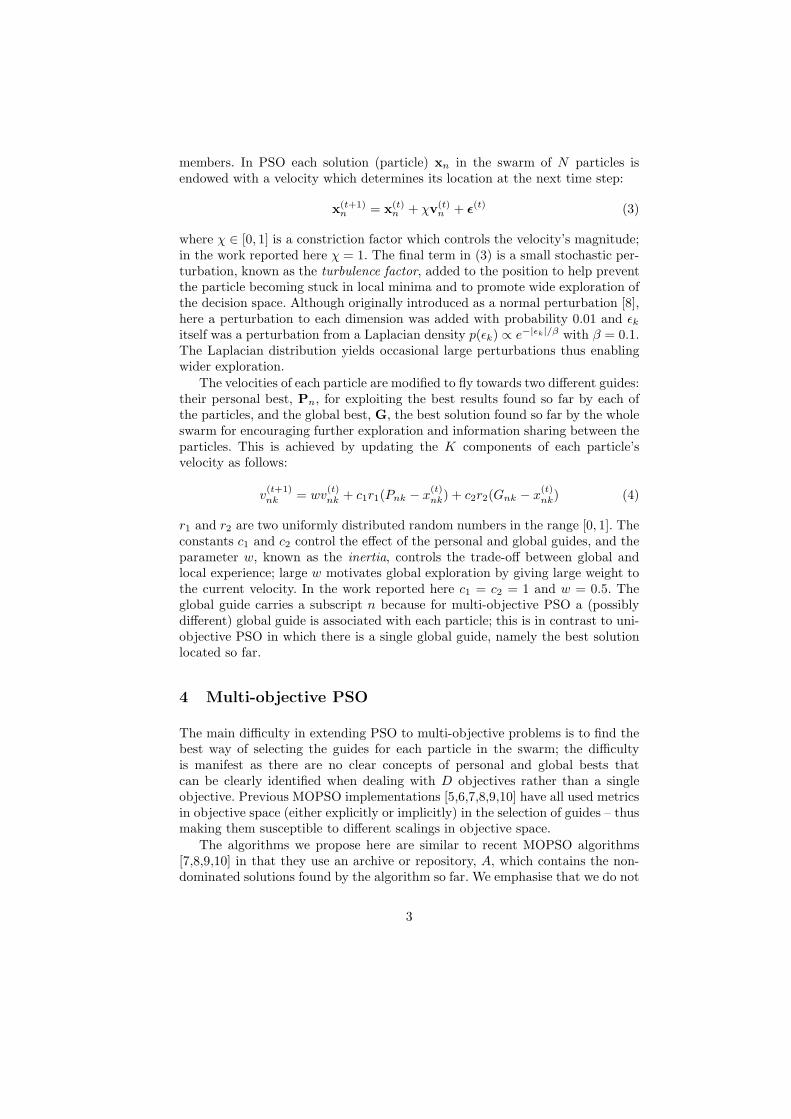
Figure 2. Archives, archive growth and histograms of distances to the DTLZ3 Paretofronts corresponding to the median result of the GD measure for (top to bottom) mt,rounds, random, prob selection methods. (The more distant clusters of particles werecut from the mt histogram for visualisation purposes.)

from the front which is quantified by GD(A). The fronts from the 20 differentruns of random and prob methods were compared pairwise by calculating thevolume in objective space dominated by one front but not by the other [12]: inover 60% of the comparisons prob outperformed random.

Figures 1 and 2 show for DTLZ1 and DTLZ3 respectively the archives,archive growth and histograms of the distances from P for the median run ac-cording to the GD measure. For both problems it is apparent that random

selection achieves tightly grouped solutions close to the true front, but the prob

scheme yields a better coverage of particles. These figures also show that theprob and random schemes both result in significantly larger archives than mt

and rounds. It is also interesting to note that although rounds often fails toconverge well it does provide good coverage; note that the rounds front shownin Figure 1 is distant from the true front giving a false impression of its coverage.

These results, along with the preference for an algorithm promoting diversity,lead us to choose prob selection as the best alternative and from now on weconcentrate on this method.

9

Table 3. Comparison, using the GD measure, between the prob and mt selectionmethods with and without scaling of objectives. ∆ indicates the percentage changebetween scaled and unscaled quantities.

prob mt

DTLZ2 unscaled rescaled ∆ unscaled rescaled ∆

Best 5.79 × 10−4 5.87 × 10−4 +1.38% 5.2 × 10−3 6.4 × 10−3 +18.75%Worst 1.10 × 10−3 9.95 × 10−4 -9.54% 0.0189 0.0174 -7.91%

Average 7.18 × 10−4 7.06 × 10−4 -1.67% 0.0113 0.0120 +5.83%Median 6.64 × 10−4 6.84 × 10−4 +2.92% 0.0111 0.0119 +6.72%S. dev. 1.44 × 10−4 1.03 × 10−4 -28.4% 3.8 × 10−3 3.1 × 10−3 -18.42%

As mentioned previously, the selection methods introduced here do not de-pend upon metric information in objective space and thus may be expected to beunaffected by the scales on which the objectives are measured. To illustrate therobustness of the method we compared 20 optimisations of the DTLZ2 test prob-lem in which one of the objectives was rescaled with 20 optimisations in whichthere was no rescaling of objectives. (All optimisations started from differentrandom initial particle locations.) On the i-th optimisation one of the objectives(chosen cyclically) for the rescaled run was multiplied by (i + 1). The frontsobtained after 45 generations were assessed using the GD(A) measure, but tofacilitate comparison the relevant objective was rescaled back to the usual scale.

Average results are shown in Table 3 and Figure 3 compares the estimatedPareto fronts for runs in which f2 was multiplied by 20 with fronts from unscaledruns. As the table shows, the optimisations using prob selection are unaffectedby the rescaling, in contrast to the mt method which relies on objective spacedistances for its selection of guides. We emphasise again that in terms of theGD metric the performance of the prob method is an order of magnitude betterthan the mt on both the scaled and unscaled problems

5 Keeping particles within the search space

The velocity and position updates (4) and (3) are liable to cause particles to ex-ceed the boundaries of the feasible regions and both single and multi-objectivePSO algorithms must be modified to keep the particles within the constraints.The manner in which this is done may have a great impact on the performanceof the algorithm as it affects the way in which particles move around the searchspace and it is particularly important when the optimum decision variables val-ues lie on or near to the boundaries. In Algorithm 1 this is delegated to theenforceConstraints function and in this section we discuss methods for ensur-ing that particles remain in the feasible region.

A number of alternatives for this have been proposed: A straightforwardmethod [10] is to truncate the location at the exceeded boundary at this gener-ation and reflect the velocity in the boundary so that the particle moves away

10

PROB MT

00.5

11.5

00.5

11.5

0

0.5

1

1.5

f1

Estimated front (equal scales)

f2

f 3

0 0.2 0.4 0.6 0.8 10

100

200

300

400

500Distances to true Pareto front (equal scales)

00.5

11.5

010

2030

0

0.5

1

1.5

f1

Estimated front (scaling f2 by 20)

f2

f 3

0 0.2 0.4 0.6 0.8 10

100

200

300

400

500

600

Distances to true Pareto front (scaling f2 by 20)

00.5

11.5

00.5

11.5

0

0.5

1

1.5

f1

Estimated front (equal scales)

f2

f 3

0 0.2 0.4 0.6 0.8 10

2

4

6

8

10

12

14Distances to true Pareto front (equal scales)

00.5

11.5

010

2030

0

0.5

1

1.5

f1

Estimated front (scaling f2 by 20)

f2

f 3

0 0.2 0.4 0.6 0.8 10

5

10

15

20

Distances to true Pareto front (scaling f2 by 20)

Figure 3. Pareto fronts and histograms of distances to the true Pareto fronts corre-sponding for unscaled (top) and with f2 rescaled by 20 (bottom) using the prob (left)and mt (right) selection rules.

at the next generation. An alternative [15] is to resample the stochastic termsin the velocity update formula (4) until a feasible position is achieved. Otherschemes rely on limiting the magnitude of the velocities, either explicitly [16] orby modifying the constriction factor χ and the other ‘constants’ w, c2 and c2

appearing in the update equations [17].Other methods may involve using a priori knowledge about the particular

problem being optimised. For example, in [9] the trespass rule for the first D−1parameters was different from the remainder [18], exploiting the knowledge thatin the DTLZ test functions the first D − 1 parameters determine the coverageof the front while the remainder determine the distance from the front. Thisapproach does improve the quality of solutions but is not used here because weare interested in examining generic methods and not those dependant on priorknowledge about the functions to be optimised.

Here we examine four methods of constraining the particles. In describingthese we assume that the constraints are constraints on individual parameters(i.e., constraints of the form L ≤ xk ≤ U for some upper and lower limits, L andU), however, they are easily generalised to oblique or curved feasible regions.

TRC Particles exceeding a boundary are truncated at the boundary for thisgeneration and the velocity is reflected in the boundary so that they tend tomove away on the next update [10].

SHR In reflecting the particle at the boundary the trc method endows theparticle at the next generation with a velocity away from the boundary, whichcan be detrimental to finding optima if the optimal decision parameters lie onthe boundary. To combat this the shr method shrinks the magnitude of thevelocity vector of the particle so that it arrives exactly at the boundary, but

11

does not alter its direction, permitting the particle to stay in the vicinity of theboundary. Suppose that the k-th component of the particle’s position exceeds aboundary at U , then the shr scheme sets

x(t+1)n = x(t)

n + σ(χv(t)n + ε) (8)

with

σ =x

(t)nk − U

χv(t)nk + εk

(9)

Note that, in contrast to the other methods discussed here, the shr schemeaffects all components of the particle’s position, rather than just the componentthat has exceeded a constraint.

RES The resampling method merely resamples the stochastic variables r1 andr2 in (4) and εk in (3) for each velocity component until the particle location isin the feasible region [15].

EXP The final method we examine updates the position component with a ran-

dom draw when that particular component, say x(t)k , would have been updated

to a position beyond a boundary at, say, b. For convenience, suppose x(t)k < U .

In this case we sample from a truncated exponential distribution oriented sothat there is a high probability of samples close to the boundary and a lower

probability of samples at the current position x(t)k . More precisely a new location

x(t+1)k is drawn with probability:

p(x(t+1)k ) ∝

exp

{

−|U−x

(t+1)k

|

|U−x(t)k

|

}

if x(t)k ≤ x

(t+1)k ≤ U

0 otherwise(10)

with obvious modifications if U < x(t)k . In a similar manner to the shr method

this scheme tends to allow particles that would have exceeded the boundaries toremain close to the boundaries.

5.1 Experiments

To determine the impact of each of the four methods, we compared the frontslocated for the DTLZ1 and DTLZ3 problems using each of them in conjunctionwith the prob guide selection scheme. The fronts were all assessed against thetrue Pareto front using the GD(A) and VP(A) measures. Each version was run20 times (using the same parameters as described above) and the results arepresented in Table 4.

It is clear that the shr method, which shrinks the velocity vector so thatthe particle arrives exactly at the boundary, yields superior results on both testproblems according to both the generational distance and volume measures.The exp method, which resamples giving preference to locations close to the

12

Table 4. Generational distance and VP (A) measures for constraint handling methodscompared on DTLZ1 & DTLZ3

GD(A) VP(A)

DTLZ1 shr res exp trc shr res exp trc

Best 3.77×10−5 1.3588 6.36 × 10−5 7 × 10−3 0.9997 0.1289 0.9996 0.9957Worst 0.0349 11.8362 0.1996 0.4706 0.9796 0 0.6958 0

Average 5.55×10−3 8.2132 0.0336 0.1747 0.9974 0.0084 0.9645 0.6983Median 1.41×10−4 8.6158 0.0178 0.2064 0.9992 0 0.992 0.8221S. dev. 0.011426 2.3872 0.05 0.147 0.0047 0.0297 0.0699 0.3035

DTLZ3

Best 5.77×10−5 21.75 2.03 × 10−4 0.0295 0.9981 0 0.9965 0.9964Worst 0.2621 41.08 1.5826 4.09 0.704 0 0 0

Average 0.0305 31.74 0.1539 1.61 0.945 0 0.8145 0.2189Median 1.52×10−3 32.29 0.0381 1.54 0.9946 0 0.9367 0.0955S. dev. 0.068707 4.25 0.3501 1.21 0.086 0 0.2892 0.2945

boundary is the next best, while the two methods that tend to move a particleaway from the boundary, trc and res, give the poorest results. Indeed res andtrc occasionally prevent convergence.

Further insight into the way in which the res and shr methods behave maybe gained by examining the trajectory of a single particle, as shown in Figure4. The figure shows 7 coordinates of a single particle during an optimisationof the DTLZ1 problem. As remarked previously, in this problem the optimumvalue for variables x3 to x7 is 0.5, while 0 ≤ x1, x2 ≤ 1 provide coverage of thefront when x3 to x7 are at their optimum value. It is clear from Figure 4 thatthe resampling method res promotes greater movements across the space whichmay be beneficial for exploration. However during the resampling the particleis pushed away from the optimal locations. In contrast the shr scheme permitsthe particle to remain close to the boundaries during the search process.

The DTLZ test problems which we analyse here are special in that the rolesof the decision variables may be clearly distinguished. However, it is likely thatin real problems optima may lie close to or on the constraint boundaries or theseregions will be visited en route to the optima and it will be important to permitparticles to properly explore these regions.

6 Conclusions

We have examined several methods of choosing global guides in multi-objectiveextensions of particle swarm optimisers. Unlike previous work, guides are se-lected without reference to distance information in the objective space, whichrenders them robust to the relative scalings of the objectives. Indeed, if the rel-ative importance or scales of the objectives were known in advance it might bemore straightforward to optimise a single, appropriately weighted, sum of the ob-jectives. Notions of dominance and Pareto optimality are well suited to handling

13

SHR RES

0 200 400 600−1

0

1

2

0 200 400 600−2

0

2

0 200 400 600−1

0

1

0 200 400 600−0.5

0

0.5

1

0 200 400 600−1

0

1

0 200 400 600−0.5

0

0.5

1

0 200 400 600−1

0

1

0 200 400 6000

500

1000

Archive Size Growth

0 200 400 600−1

0

1

0 200 400 6000

0.5

1

0 200 400 600−2

−1

0

1

0 200 400 600−0.5

0

0.5

1

0 200 400 600−0.5

0

0.5

1

0 200 400 600−0.5

0

0.5

1

0 200 400 600−0.5

0

0.5

1

0 200 400 6000

50

100

150

Archive Size Growth

Figure 4. Movements of a particle and growth of the archive during the searchingprocess when using shr and res methods on DTLZ1. (x1 to x7 are shown top-left,top-right, . . . , to bottom-right.)

competing objectives whose relative importance is a priori unknown and it istherefore natural to eschew metric information in favour of dominance conceptswhen choosing guides. We find that selecting guides probabilistically from thearchive of non-dominated solutions, giving more weight to solutions that dom-inate few particles, provides both good convergence and widespread coverage.This method yields superior performance to an existing MOPSO technique andis robust to changes of scale in the objective functions.

The computation involved in the selection is a more extensive than otherrecently proposed schemes (e.g., [9,10]) but is more than compensated for byimproved convergence and coverage.

The prob selection method selects guides with probability inversely propor-tional to the number of particles the potential guide dominates (c.f., (6)). Itwould be interesting to examine the performance of an algorithm which selectsguides with probability proportional to |Xa|

−q; as q → 0 the method becomesthe random method, but as q increases additional weight is given to sparse re-gions. Although this might enable finer control of the convergence and coverageit would introduce an additional parameter to be ‘tweaked’.

It was found that the manner in which particles are constrained to the fea-sible region can vastly affect the performance of a MOPSO. Four methods ofconstraining particles were examined and it was found that a method whichpermits particles to remain close to the boundaries enables more rapid locationof the Pareto front. We anticipate that careful handling of solutions to allowexploration close to the boundaries will be important not only in MOPSO, butalso in other approaches to multi-objective optimisation.

14

References

1. Srinivas, N., Deb, K.: Multiobjective Optimization Using Nondominated Sortingin Genetic Algorithms. IEEE Transactions on Evolutionary Computation 2(3)(1995) 221–248

2. Zitzler, E., Thiele, L.: Multiobjective Evolutionary Algorithms: A ComparativeCase Study and the Strength Pareto Approach. IEEE Transactions on Evolution-ary Computation 3(4) (1999) 257–271

3. Laumanns, M., Zitzler, E., Thiele, L.: A Unified Model for Multi-Objective Evo-lutionary Algorithms with Elitism. In: Proceedings of the 2000 Congress on Evo-lutionary Computation. (2000) 46–53

4. Kennedy, J., Eberhart, R.: Particle Swarm Optimization. In: Proceedings of theFourth IEEE International Conference on Neural Networks. (1995) 1942–1948

5. Hu, X., Eberhart, R.: Multiobjective Optimization Using Dynamic NeighborhoodParticle Swarm Optimization. In: Proceedings of the 2002 Congess on EvolutionaryComputation, IEEE Press (2002)

6. Parsopoulos, K., Vrahatis, M.: Particle Swarm Optimization Method in Multi-objective Problems. In: Proceedings of the 2002 ACM Symposium on AppliedComputing (SAC 2002). (2002) 603–607

7. Coello, C., Lechunga, M.: MOPSO: A Proposal for Multiple Objective ParticleSwarm Optimization. In: Proceedings of the 2002 Congress on Evolutionary Com-putation, IEEE Press (2002) 1051–1056

8. Fieldsend, J., Singh, S.: A Multi-Objective Algorithm based upon Particle SwarmOptimisation, an Efficient Data Structure and Turbulence. In: Proceedings of UKWorkshop on Computational Intelligence (UKCI 02). (2002) 37–44

9. Mostaghim, S., Teich, J.: Strategies for Finding Good Local Guides in Multi-Objective Particle Swarm Optimization (MOPSO). In: IEEE 2003 Swarm Intelli-gence Symposium. (2003) 26–33

10. Coello, C., Pulido, G., Lechunga, M.: Handling Multiple Objectives with Parti-cle Swarm Optimization. IEEE Transactions on Evolutionary Computation 8(3)(2004) 256–279

11. Hanne, T.: On the convergence of multiobjective evolutionary algorithms. Euro-pean Journal of Operational Research 117 (1999) 553–564

12. Fieldsend, J., Everson, R., Singh, S.: Using Unconstrained Elite Archives forMulti–Objective Optimisation. IEEE Transactions on Evolutionary Computation7 (2003) 305–323

13. Deb, K., Thiele, L., Laumanns, M., Zitzler, E.: Scalable Multi–Objective Opti-mization Test Problems. In: Congress on Evolutionary Computation (CEC’2002).Volume 1. (2002) 825–830

14. Veldhuizen, D.V., Lamont, G.: Multiobjective Evolutionary Algorithms Research:A History and Analysis. Technical Report TR-98-03, Dept. Elect. Comput. Eng.,Graduate School of Eng., Air Force Institute Technol., Wright-Patterson AFB, OH(1998)

15. Fieldsend, J.: Multi–Objective Particle Swarm Optimization Methods. TechnicalReport No. 419, Department of Computer Science, University of Exeter (2004)

16. van den Bergh, F.: An Analysis of Particle Swarm Optimizers. PhD thesis, Facultyof Natural and Agricultural Science, University of Pretoria (2001)

17. Clerc, M.: The Swarm and the Queen: Towards a Deterministic and AdaptativeParticle Swarm Optimization. In: Proceedings of the Congress on EvolutionaryComputation, IEEE Press (1999) 1951–1957

18. Mostaghim, S., Teich, J.: Personal communication. (2004)

15