A Monetary Policy Regime Whose Time Has Come and Gone

INFLATION TARGETING A Monetary Policy Regime Whose Time Has

Come and Gone

David Beckworth

MERCATUS RESEARCH

Bridging the gap between academic ideas and real-world problems

http://mercatus.org/

Copyright © 2014 by David Beckworth and the Mercatus Center at George Mason University

Mercatus Center at George Mason University3434 Washington Boulevard, 4th FloorArlington, VA 22201(703) 993-4930mercatus.org

Release date: July 10, 2014

ABOUT THE MERCATUS CENTER AT GEORGE MASON UNIVERSITY

The Mercatus Center at George Mason University is the world’s premier university source for market-oriented ideas—bridging the gap between academic ideas and real-world problems.

A university-based research center, Mercatus advances knowledge about how markets work to improve people’s lives by training graduate students, conduct-ing research, and applying economics to offer solutions to society’s most pressing problems.

Our mission is to generate knowledge and understanding of the institutions that affect the freedom to prosper and to find sustainable solutions that overcome the barriers preventing individuals from living free, prosperous, and peaceful lives.

Founded in 1980, the Mercatus Center is located on George Mason University’s Arlington campus.

www.mercatus.org



ABOUT THE AUTHOR

David Beckworth is a former international economist at the US Department of the Treasury and the author of Boom and Bust Banking: The Causes and Cures of the Great Recession. His research focuses on monetary policy, and his work has been cited by the Wall Street Journal, the Financial Times, the New York Times, Bloomberg Businessweek, and the Economist. He has advised congressional staffers on monetary policy and has written for Barron’s, Investor’s Business Daily, the New Republic, the Atlantic, and National Review. Currently he is an assistant professor at Western Kentucky University.

MERC ATUS CENTER AT GEORGE M A SON UNIVER SIT Y

4

ABSTRACT

Inflation targeting emerged in the early 1990s and soon became the dominant monetary-policy regime. It provided a much-needed nominal anchor that had been missing since the collapse of the Bretton Woods system. Its arrival coincided with a rise in macroeconomic stability for numerous countries, and this led many observ-ers to conclude that it is the best way to do monetary policy. Some studies show, however, that inflation targeting got lucky. It is a monetary regime that has a hard time dealing with large supply shocks, and its arrival occurred during a period when they were small. Since this time, supply shocks have become larger, and inflation targeting has struggled to cope with them. Moreover, the recent crisis suggests it has also has a tough time dealing with large demand shocks, and it may even contribute to financial instability. Inflation targeting, therefore, is not a robust monetary-policy regime, and it needs to be replaced.

JEL codes: E44, E52, E58

Keywords: inflation targeting, financial stability, total dollar spending target, sup-ply shocks, Great Inflation, monetary stability, nominal anchor

5

I. INTRODUCTION

One of the great macroeconomic accomplishments over the past thirty years has been the eradication of the high inflation that arose in the 1970s. This “Great Inflation” was endemic to most advanced economies and is generally attributed to monetary-policy failures.1 The conquest of this inflation was achieved by monetary authorities recognizing their role in creating price stability and adopting policies that promoted it. In the United States this effort began in 1979 with the appointment of Paul Volker as the chair of the Federal Reserve. Over the next few years he led an intense battle against inflation that included two recessions as casualties. His efforts led to a decline in trend inflation over the next decade. Similar efforts were made in other advanced economies.

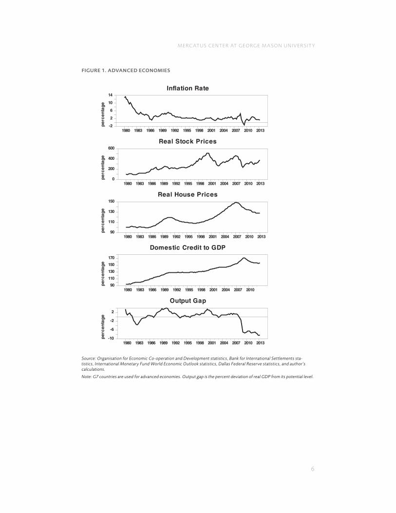
The main monetary regime to emerge in this long battle over inflation was infla-tion targeting. This approach firmly committed central banks to a stable inflation rate, usually around 2 percent. Most advanced economies adopted some form of inflation targeting over the past three decades and during this time saw their infla-tion rates fall, as seen in the top panel of figure 1.2 Inflation targeting was heralded as a great success by many observers.3

But just as the successes of inflation targeting were becoming clear, so were its limits. An unsustainable boom in stock prices in the late 1990s, followed by a similar surge in housing prices and credit growth in the first few years after 2000, occurred despite the increased price stability. These developments occurred for most advanced economies, as indicated by figure 1. The housing and credit boom, in particular, stirred much soul-searching on the limits of inflation targeting, even

1. Michael Bordo and Athanasios Orphanides, The Great Inflation: The Rebirth of Modern Central Banking (Chicago: University of Chicago Press, 2013).2. In some cases, the adoption of an inflation target was implicit—as in the case of the United States. This point is discussed in section 2.3. For example, see Ben Bernanke, T. Laubach, F. S. Mishkin, and A. S. Posen, Inflation Targeting: Lessons from the International Experience (Princeton, N.J.: Princeton University Press, 1999); Frederick Mishkin and Klaus Schmidt-Hebbel, “Does Inflation Targeting Make a Difference?” (NBER Working Paper No. 12876, 2007); and Carl Walsh, “Inflation Targeting: What Have We Learned?” International Finance 12, no. 2 (2009): 195–233.


6

Inflation Rate

perc

enta

ge

1980 1983 1986 1989 1992 1995 1998 2001 2004 2007 2010 2013-2

2

6

10

14

Real Stock Prices

perc

enta

ge

1980 1983 1986 1989 1992 1995 1998 2001 2004 2007 2010 20130

200

400

600

Real House Prices

perc

enta

ge

1980 1983 1986 1989 1992 1995 1998 2001 2004 2007 2010 201390

110

130

150

Domestic Credit to GDP

perc

enta

ge

1980 1983 1986 1989 1992 1995 1998 2001 2004 2007 201090

110130150170

Output Gap

perc

enta

ge

1980 1983 1986 1989 1992 1995 1998 2001 2004 2007 2010 2013-10

-6

-2

2

FIGURE 1. ADVANCED ECONOMIES

Source: Organisation for Economic Co-operation and Development statistics, Bank for International Settlements sta-tistics, International Monetary Fund World Economic Outlook statistics, Dallas Federal Reserve statistics, and author’s calculations.

Note: G7 countries are used for advanced economies. Output gap is the percent deviation of real GDP from its potential level.


7

among its most ardent advocates. Some observers concluded that central banks should modify their policy rules so that they would also respond to swings in asset prices.4 Others argued that monetary authorities should instead focus more intently on pushing macroprudential policies.5 In both cases, though, inflation targeting was to be, not terminated, but enhanced with more vigilant central-bank focus on asset prices and credit growth.

Another set of observers questioned whether inflation targeting itself needed to be reconsidered. These individuals began wondering if an environment of price stability was the primordial soup from which emerged financial instability.6 They noted that positive supply shocks, which were abundant during this time, created problems for central banks that targeted inflation. On the one hand, the positive supply shocks coming from technology gains and the opening up of Asia meant more robust economic growth. On the other hand, the positive supply shocks meant sustained, downward pressure on inflation that, if not offset, would push inflation below its target. Central banks could prevent the too-low inflation by lowering their policy interest rates. This response, however, had the potential to further fuel the supply-side driven recovery and cause the economy to grow too fast. These developments, in turn, might create excess optimism, lower risk pre-miums, and spark increased leverage by firms and households. In short, large and frequent supply shocks can be a real challenge for inflation-targeting central banks. According to some, this was the backstory to the financial-sector boom leading up to the Great Recession.7

Another limitation of inflation targeting that became apparent during the Great Recession was its inability to return economies to their full potential. This inabil-ity surprised many observers, because inflation targeting seemed to have worked well at maintaining full employment during the two decades leading up to the 2007 recession. The Great Recession, however, showed that large output gaps—devia-tions of real GDP from its full potential—can persist, as seen in figure 1. Output gaps,

4. Stephen Cecchetti, Hans Genberg, and Sushil Wadhwani, “Asset Prices in a Flexible Inflation Targeting Framework,” in Asset Price Bubbles: Implications for Monetary, Regulatory, and International Policies, ed. William C. Hunter, George G. Kaufman, and Michael Pomerleano (Cambridge, MA: MIT Press, 2002); Kevin J. Lansing, “Monetary Policy and Asset Prices,” Federal Reserve Bank of San Francisco Economic Letter 34 (2008).5. Donald Kohn, Speech at the 26th Cato Institute Monetary Policy Conference, Washington, DC, 2008; Claudio Borio, “The Macroprudential Approach to Regulation and Supervision,” VoxEU, April 14, 2009, http://www.voxeu.org/article/we-are-all-macroprudentialists-now.6. Claudio Borio and Philip Lowe, “Asset Prices, Financial and Monetary Stability: Exploring the Nexus” (BIS Working Paper No. 114, 2002); William R. White, “Is Price Stability Enough?” (BIS Working Paper No. 205, 2006).7. David Beckworth, “Aggregate Supply-Driven Deflation and Its Implications for Macroeconomic Stability,” Cato Journal 25, no. 3 (2008): 363–84; George Selgin, David Beckworth, and Berrak Bahadir, “The Productivity Gap: Monetary Policy, the Subprime Boom, and the Post-2001 Productivity Surge” (working paper, University of Georgia, 2013).

http://www.voxeu.org/article/we-are-all-macroprudentialists-now


8

by definition, are the result of demand shocks that push the economy away from full employment. This implies that the large output gap that emerged during the Great Recession was the result of large demand shocks over 2007–2009. It also implies that inflation targeting is not an adequate response to large demand shocks.

Some commentators pointed out there was more to the sizable output gap than the large demand shocks, because behind the latter was a problem of excess money demand.8 Such a problem occurs when desired money balances exceed actual money holdings and, in turn, cause individuals and firms to rebalance their portfolios away from risky assets toward safe, liquid ones. Collectively, this rebalancing lowers asset prices, increases risk premiums, and ultimately reduces aggregate spending. Inflation targeting’s inability, then, to restore full employment was a result of its inability to resolve the problem of excess money demand during this time.

A final shortcoming of inflation targeting is that it requires judgment calls. This is because over time inflation targeting in practice has become flexible inflation targeting. Under this approach, the 2 percent inflation target is no longer a short-run target, but a medium-run one. This allows central banks to have flexibility in the short run to deal with economic shocks that push the economy away from full employment. It also means, though, that monetary policymakers have to know in real time whether changes in inflation and real GDP are being caused by demand shocks or supply shocks. Central banks are capable of responding in a productive manner to the former, but not the latter. Judgment calls, sometimes bad ones, are an inevitable result. Many believe that a bad judgment call occurred between 2003 and 2004, when the Federal Reserve lowered its target interest rate to 1 percent because of concerns about deflation, despite the strong growth in housing and credit—or in September 2008, when the Federal Reserve decided against lowering its target interest rate because of inflation concerns, even though the US economy was sharply contracting at this time.

These problems suggest that inflation targeting may have reached its expira-tion date. It served a purpose in the long battle against the great inflation of the 1970s, but now that its limits are better known some critics are calling for a new monetary regime.9 Others, as noted above, want to keep inflation targeting but enhance it with more focus on asset price and credit growth. In this paper, I take a closer look at inflation targeting, including its history, successes, and problems. I too conclude that inflation targeting’s time has come and gone. The global economy

8. Nicholas Rowe, “A Global Liquidity Crisis,” in Boom and Bust Banking: The Causes and Cures of the Great Recession, ed. David Beckworth (Oakland, CA: Independent Institute, 2012); William Woolsey, “The Great Recession and Monetary Disequilibrium,” in Boom and Bust Banking: the Causes and Cures of the Great Recession, ed. David Beckworth (Oakland, CA: Independent Institute, 2012).9. Scott Sumner, “Retargeting the Fed,” National Affairs 9 (2011): 79–96; David Beckworth and Ramesh Ponnuru, “Monetary Regime Change: An Old Order Fails,” National Review, June 11, 2012, 33–35; and Jeffrey Frankel, “The Death of Inflation Targeting,” VoxEU, June 19, 2012, http://www.voxeu.org/article /inflation-targeting-dead-long-live-nominal-gdp-targeting.

http://www.voxeu.org/article/inflation-targeting-dead-long-live-nominal-gdp-targeting

http://www.voxeu.org/article/inflation-targeting-dead-long-live-nominal-gdp-targeting


9

has become so financially developed and integrated that any monetary policy that aims for inflation targeting, even over the medium term, will be planting the seeds of a future financial crisis. Price stability is not enough. It is time to retarget mon-etary policy.

II. HISTORY OF INFLATION TARGETING

The origins of inflation targeting can be traced back to the high inflation of the late 1970s and early 1980s. This “Great Inflation,” which reached double digits in many advanced economies, emerged in the vacuum created by the collapse of the Bretton Woods system.10 For many decades the Bretton Woods system had provided a nominal anchor—a money-denominated measure that is pinned down in order to keep the price level stable—through its fixed exchange rates. Its collapse in the early 1970s created a void that, in conjunction with bad economic theories, measure-ment problems, and political pressures for low unemployment led to the high infla-tion that followed.11 The Great Inflation eventually forced monetary authorities in advanced economies to recognize their policies’ shortcomings and seek out a new, credible nominal anchor.

The first nominal anchor they tried was money-supply targeting. The idea was to constrain the growth of money so as to keep total money spending stable. By the end of the 1970s many advanced economies had tried it in some form. The Federal Reserve, for example, began setting target growth rates for the M1 money supply in the mid-1970s and in 1979 began targeting nonborrowed bank reserves.12 The success of money-supply targeting depended on the existence of a stable relationship between the quantity of money and total money spending. This relationship, however, appeared to break down during this time as financial innovations and the relaxing of certain regulations created an unstable demand

10. The Great Inflation for the US economy is usually attributed to the 1965–1982 period. The really high and unstable inflation, though, emerged in the late 1970s and early 1980s. See Allan Meltzer, “The Great Inflation,” Federal Reserve Bank of St. Louis Review (March/April 2005): 145–76.11. There were two bad economic theories. First, there was a belief by some policymakers in a permanent trade-off between unemployment and inflation, or a long-run Phillips Curve. Second, many economists believed monetary policy did not matter for inflation. Inflation, instead, was controlled by “incomes poli-cies” and other forms of fiscal policy. See Christina Romer, “Commentary on the Great Inflation,” Federal Reserve Bank of St. Louis Review 87, no. 2 (March/April 2005): 177–186; and Daniel Thorton, “How Did We Get to Inflation Targeting and Where Do We Go Now? A Perspective from the US Experience,” Federal Reserve Bank of St. Louis Review 94, no. 1 (January/February 2012): 65–81. The measurement problem, as argued by Athanasios Oprhanides, was that Fed officials did not know the true productive capacity in real time and consequently conducted inappropriate monetary policy. See Orphanides, “The Quest for Prosperity without Inflation,” Journal of Monetary Economics 50, no. 3 (2003): 633–63.12. Nonborrowed bank reserves are reserves that banks obtain through open-market operations with the Federal Reserve. Bank reserves plus currency make up the monetary base.


10

for money.13 By the mid-1980s, the consensus among monetary authorities was that money-supply targeting was not an effective nominal anchor.14 The search was on for another one.

A number of European countries in the 1980s moved back toward a fixed-exchange-rate regime for their nominal anchor. This was known as the European Monetary System, and it had the German mark as the anchor currency. This meant the German central bank, the Bundesbank, would effectively be setting monetary policy for Western Europe. This development was important for two reasons. First, the Bundesbank effectively became an inflation targeter during this time, even though it officially targeted the money supply. Over time, it developed a policy where an inflation target was set and then a quantity-theory equation was used to back out the implied monetary-growth target. The Bundesbank’s money-supply targets were flexible and often missed when they conflicted with other economic goals, particularly inflation.15 One study found that when “conflicts arose between its money growth targets and inflation targets, the Bundesbank generally chose to give greater weight to its inflation targets.”16 This pragmatic approach taken by the Bundesbank was very successful and is viewed by some, like Ben Bernanke, as a seminal case of flexible inflation targeting, the experience of which helped shape the first official inflation-targeting central banks.17

13. For example, the creation of money-market mutual funds, which were highly liquid and paid mar-ket interest rates, pulled funds out of traditional bank deposits. That meant the M1 money supply, which includes checking accounts but not money-market mutual funds, became a less reliable predic-tor of total dollar spending. Similarly, the Garn-St. Germain Depository Institution Act of 1982 autho-rized money-market deposit accounts that are counted in M2, but not M1. This further eroded the rela-tionship between M1 and total dollar spending. For more, see Pedro Teles and Ruilin Zhou, “A Stable Money Demand: Looking for the Right Monetary Aggregate,” Federal Reserve Bank of Chicago Economic Perspectives 29, no. 1 (2005): 50–63.14. Some observers contend the problem was not money-supply targeting per se, but the fact that mon-etary authorities were using crude measures of money in their targets. Standard money measures like M1 and M2 are “simple sum” indicators that treat all the component money assets as perfect substitutes. For example, M2 includes cash, checking, saving and time deposits, and retail money market funds. Critics note that these money assets are not perfect substitutes and should be weighted accordingly. They believe that if the assets were weighted properly, the unstable money-demand relationship would disappear and money-supply targeting could once again serve as a reliable nominal anchor. For more on this point, see Joshua Hendrickson, “Redundancy or Mismeasurement: A Reappraisal of Money,” Macroeconomic Dynamics (forthcoming).15. For more on Germany’s monetary targeting regime, see Frederick Mishkin, “From Monetary Targeting to Inflation Targeting: Lessons from the Industrialized Countries,” in Banco de Mexico, Stabilization and Monetary Policy: The International Experience (Mexico City: Bank of Mexico, 2002).16. Ben Bernanke and I. Mihov, “What Does the Bundesbank Target?,” European Economic Review 41 (1997): 1025–53.17. The central bank of Switzerland also was relatively successful in taming inflation using money-supply targeting during this time. Ben Bernanke, therefore, also points to it as a seminal flexible-inflation tar-geter. Its performance, however, was not as consistent as the Bundesbank. Ben Bernanke, “A Perspective on Inflation Targeting” (speech, Annual Washington Policy Conference of the National Association of Business Economists, 2003); Thorton, How Did We Get to Inflation Targeting.


11

The second reason the European Monetary System mattered to the history of the inflation targeting is that it spawned the first of several exchange crises in the 1990s, which painfully demonstrated how hard it is to use exchange-rate pegs as a nominal anchor. Germany’s economy was on a very different track than the rest of Europe in the early 1990s. It was overheating while the rest of Europe was slowing down. So when the Bundesbank tightened during this time, it meant the European countries pegged to its currency would also face tighter monetary con-ditions. For the United Kingdom and Italy, whose economies were already weak, this was too high a cost and they left the EMS.18 Similar exchange-rate crises took place in Mexico in 1994 and a number of other emerging economies in the late 1990s. They too found that using exchange-rate pegs as a nominal anchor came at too high a cost.

The failure of fixed-exchange regimes in the 1990s coincided with the early adop-tion of inflation targeting as the new nominal anchor. The first two countries to officially implement inflation targeting were New Zealand and Canada in the early 1990s. Taking lessons from the Bundesbank’s experience, these countries adopted inflation targets of about 2 percent a year and gave their central banks independence in pursuit of this target. They also attempted to clearly communicate their infla-tion targets to the public. Soon after, the United Kingdom, Sweden, and Australia adopted similar policies. Spurred by the success of these early adopters and the failures of exchange-rate pegs as nominal anchors, a number of other countries adopted inflation targeting over the next few decades. There are now almost 30 official inflation-targeting central banks.19

The early adopters of inflation targeting were focused solely on price stability. Over time, though, inflation targeting became more flexible so that price stability became a medium-term goal. That is, central banks would aim to hit their inflation target on average over a 2–5 year period.20 This so-called flexible-inflation-targeting approach allows central bankers to respond to “output gaps” (deviations of real GDP from its full employment level) in the short run while still anchoring long-term inflation expectations. Bernanke called this approach “constrained discretion” because it combined “short-run policy flexibility with the discipline imposed by the medium-term inflation target.”21

18. Other countries that stayed in the European Monetary System had to significantly devalue their currencies.19. For a full list of inflation targeters, see Gill Hammond, State of the Art Inflation Targeting, CCBS Handbook No. 29 (London: Centre for Central Banking Studies, Bank of England, 2012), http://www .bankofengland.co.uk/education/Documents/ccbs/handbooks/pdf/ccbshb29.pdf.20. Central banks with less-anchored inflationary expectations would aim for the low end of the 2–5-year range, while a credible central bank with well-anchored inflationary expectations would aim for the long end of the range.21. Ben Bernanke, “The Effects of the Great Recession on Central Bank Doctrine and Practice” (speech, Federal Reserve Bank of Boston 56th Economic Conference, 2011).

http://www.bankofengland.co.uk/education/Documents/ccbs/handbooks/pdf/ccbshb29.pdf

http://www.bankofengland.co.uk/education/Documents/ccbs/handbooks/pdf/ccbshb29.pdf


12

The Federal Reserve is a good example of a flexible-inflation-targeting central bank. Officially, it only became an inflation targeter in 2012, but for many years it has had a dual mandate of price stability and full employment. Though it too succumbed to the Great Inflation, most studies indicate that by the early 1990s the Federal Reserve was implicitly targeting an inflation rate around 2 percent and was systematically responding to output gaps.22 Former Federal Reserve chairman Ben Bernanke acknowledged these facts in a 2011 speech: “As a practical matter, the Federal Reserve’s policy framework has many of the elements of flexible inflation targeting . . . the Federal Open Market Committee (FOMC) is committed to stabiliz-ing inflation over the medium run while retaining the flexibility to help offset cyclical fluctuations in economic activity and employment.”23 Like the Federal Reserve, most inflation-targeting central banks today operationally are flexible inflation targeters.

To be clear, flexible inflation targeting does not mean central banks will system-atically try to exploit some kind of Phillips curve relationship. They learned the futility of attempting this in the 1970s. Rather, inflation concerns will still trump output gap concerns if monetary authorities believe responding to the latter will jeopardize medium-term price stability. For example, Federal Reserve Chairman Ben Bernanke in 2009 said that despite the 10 percent unemployment rate the Fed would not raise its inflation target, because doing so might jeopardize its inflation-fighting credibility.24 Similarly, in spite of the ongoing eurozone crisis, the European Central Bank raised its target interest rate twice in 2011 because of inflation concerns. Flexible inflation targeting, then, is ultimately about creating a nominal anchor.

III. THE ACCOMPLISHMENTS OF INFLATION TARGETING: TRUE SUCCESS OR LUCK?

So what has inflation targeting accomplished? As noted above, the emergence of inflation targeting coincided with the anchoring of inflation rates around 2 percent in advanced economies. Ostensibly, then, it has accomplished the objective of cre-ating a credible nominal anchor to fill the void left by the collapse of the Bretton

22. Peter Ireland finds that the Fed’s implicit inflation target finally settled around 2 percent in 1993, and James Stock and Mark Watson find similar declines in observed inflation volatility around this time. See Ireland, “Changes in the Fed’s Inflation Target: Causes and Consequences,” Journal of Money, Credit, and Banking 39, no. 8 (2007): 1851–81; and Stock and Watson, “Modeling Inflation after the Crisis,” Federal Reserve Bank of Kansas City Economic Policy Symposium 2010, 173–220. John B. Taylor in his famous study finds that the Fed was systematically responding to the output gap and deviations of inflation from 2 percent by this time. See Taylor, “Discretion versus Policy Rules in Practice,” Carnegie-Rochester Conference Series on Public Policy 39 (1993): 195–214.23. Bernanke, “Effects of the Great Recession.”24. Sudeep Reddy, “Sen. Vitter Presents End-of-Term Exam for Bernanke,” Real Time Economics Blog, Wall Street Journal, December 17, 2009, http://blogs.wsj.com/economics/2009/12/17/sen-vitter -presents-end-of-term-exam-for-bernanke/.

http://blogs.wsj.com/economics/2009/12/17/sen-vitter-presents-end-of-term-exam-for-bernanke/

http://blogs.wsj.com/economics/2009/12/17/sen-vitter-presents-end-of-term-exam-for-bernanke/


13

Woods system. Several studies looking at a large sample of inflation-targeting countries across several decades find evidence to support this interpretation.25 They find that inflation-targeting countries generally experienced a firming of long-run inflation expectations, a lowering of exchange-rate pass through, increased central-bank independence, and improved monetary-policy efficiency in terms of minimiz-ing a trade-off between inflation and output volatility.26

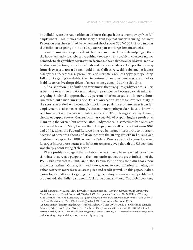
Figure 2 provides one example of these accomplishments. Using data from the Philadelphia Federal Reserve’s Survey of Professional Forecasters, it shows how flexible inflation targeting in the United States led to the reanchoring of the 10-year average inflation forecast in the 1990s. Remarkably, the large run-up of the Fed’s balance sheet since 2008 has not significantly altered long-run inflation expec-tations. This speaks to the inflation-fighting credibility the Federal Reserve has earned using flexible inflation targeting as a nominal anchor.27

FIGURE 2. EXPECTED AVERAGE ANNUAL US INFLATION RATE

Source: Philadelphia Federal Reserve Quarterly Survey of Forecasters database.

25. Stephen Cecchetti and Michael Ehrmann, “Does Inflation Targeting Increase Output Volatility? An International Comparison of Policymakers’ Preferences and Outcomes,” in Monetary Policy: Rules and Transmission Mechanism, ed. Norman Loayza and Klaus Schmidt-Hebbel, Proceedings of the Fourth Annual Conference of the Central Bank of Chile (2002); Stephen Cecchetti, Alfonso Flores-Lagunes, and Stefan Krause, “Has Monetary Policy Become More Efficient? A Cross-Country Analysis,” Economic Journal 116, no. 511 (April 2006): 408–33; Mishkin and Schmidt-Hebbel, “Does Inflation Targeting Make a Difference?”; Walsh, “Inflation Targeting.”26. These accomplishments were found to be even more pronounced for developing economies that adopted flexible inflation targeting.27. Similar long-run inflation forecasts are found by taking the difference between treasury inflation-protected securities and regular treasury securities. This method shows more volatility, but it indicates a long-run inflation forecast of about 2.5 percent.

Expected Average Annual U.S. Inflation Rate10-Year Forecast

percentage

1992 1995 1998 2001 2004 2007 2010 20132.00

2.25

2.50

2.75

3.00

3.25

3.50

3.75

4.00


14

Despite these accomplishments, the above studies note that the success of infla-tion targeting depends on supply shocks being few and small. Supply shocks come from fundamental changes to economy. The introduction of a new technology that lowers firms’ per-unit production costs or a sudden reduction in the supply of an important input like oil are examples of supply shocks. These shocks create prob-lems for monetary policy because they push real GDP and the price level in oppo-site directions. A technology innovation, for example, would tempt an inflation-targeting central bank to ease monetary policy, because the resulting productivity gains would lower costs and put downward pressure on output prices. Doing so, however, may add excessive monetary stimulus to the technology-driven economic gains and create an unsustainable economic boom. Alternatively, a sudden reduc-tion in the global supply of oil would raise output prices and might tempt a central bank to tighten monetary policy. Tightening, though, would inflict even more harm on an economy already weakened by the reduction in the oil supply.

Demand shocks, on the other hand, push real GDP and the price level in the same direction and are therefore easier for an inflation-targeting central bank to handle. Moreover, monetary policy’s influence on the economy comes from altering demand via its influence on monetary conditions. It is well suited to offset unwanted demand shocks. For example, imagine there were a sudden surge in consumer spending that led to an unsustainable increase in real GDP and an above-target rate of inflation. An inflation-targeting central bank responding to the higher inflation would also be simultaneously responding to the higher-than-desired growth in real GDP when it tightened monetary policy. Inflation targeting, then, works best when demand shocks are the main drivers of the business cycle.28

Figure 3 shows for the US economy the estimated effect of the typical supply and demand shocks on real GDP and the price level for the period from the first quarter of 1950 to the second quarter of 2013.29 The black lines show the average response to these shocks in percentage terms and the dashed lines provide a 90 percent confi-dence interval. This figure shows that the typical positive supply shock permanently raised the level of real GDP and permanently lowered the price level. The typical positive demand shock, however, only temporarily raised real GDP but permanently raised the price level. Negative supply and demand shocks of the same size would create mirror-opposite responses to the ones in the figures.

28. As noted later in this paper, it actually depends on there being small demand shocks. Large demand shocks can create insurmountable problems for inflation targeting.29. These estimates come from a vector autoregression (VAR) that includes real GDP and the PCE price-level measure. It uses long-run identifying restrictions such that shocks to real GDP are allowed to per-manently affect real GDP and the price level, while shocks to the price level can temporarily affect real GDP and permanently affect the price level. These restrictions allow me to identify the real GDP shocks as supply shocks and the price-level shocks as demand shocks. The model is estimated using quarterly data and six lags (enough to whiten the residuals), and in growth-rate form. The figures show the cumu-lated responses or level responses to the shocks.


15

FIGURE 3. TYPICAL RESPONSES TO SUPPLY AND DEMAND SHOCKS: US ECONOMY, 1950:Q1–2013:Q2

Source: Federal Reserve Economic Data database and author’s calculations.

Note: Black lines are point estimates and dashed lines are 90% confidence intervals.

So, what is an inflation-targeting central bank to do with such supply shocks? One answer it that is can hope that it does not get many supply shocks. In short, it can hope to be lucky. Some studies of inflation targeting have questioned whether the Federal Reserve and other advanced economies’ central banks were, in fact, lucky in the decades leading up to the Great Recession. While acknowledging that flexible inflation targeting has provided a nominal anchor, these studies point to the reduced frequency of supply shocks in this period as the reason it worked out so well. For example, Stephen Cecchetti and Michael Ehrmann note that “supply shocks, which move output and inflation in opposite directions and force monetary policymakers to make choices, may have been on average smaller (in absolute value) during the 1990s.”30 Likewise, Frederick Mishkin and Klaus Schmidt-Hebbel conclude that for the 1989–2004 period “industrial inflation targeters improve their macroeconomic performance only because they face smaller supply shocks.”31 Carl Walsh takes an even more skeptical view, attributing the successful adoption of inflation targeting to “good luck” coming from a “benign economic environment.”32

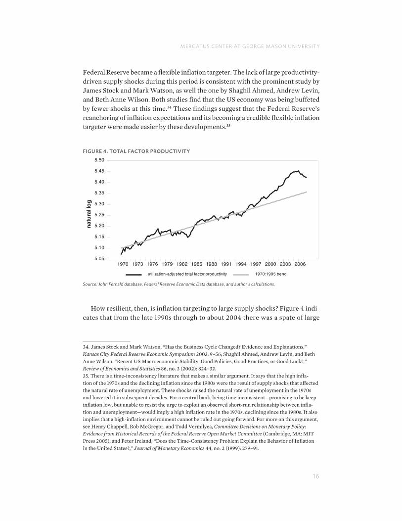
Figure 4 lends support to this “good luck” view, at least for the US economy. It plots utilization-adjusted total factor productivity, a measure of overall productivity that controls for swings in the business cycle.33 This figure indicates that productiv-ity growth was relatively stable between the mid-1980s and mid-1990s, the years the

30. Cecchetti and Ehrmann, “Does Inflation Targeting Increase Output Volatility?,” 252.31. Mishkin and Schmidt-Hebbel, “Does Inflation Targeting Make a Difference?,” 26.32. Walsh, “Inflation Targeting,” 216.33. Headline productivity tends to be procyclical, owing to existing labor and capital working more intensely during booms and less intensely during busts. To properly measure changes in productivity, then, one must control for these changes in utilization of labor and capital.

Price Level Response

Real GDP Response

Supply Shock Demand Shock

Quarters after Shock Quarters after Shock


16

Federal Reserve became a flexible inflation targeter. The lack of large productivity-driven supply shocks during this period is consistent with the prominent study by James Stock and Mark Watson, as well the one by Shaghil Ahmed, Andrew Levin, and Beth Anne Wilson. Both studies find that the US economy was being buffeted by fewer shocks at this time.34 These findings suggest that the Federal Reserve’s reanchoring of inflation expectations and its becoming a credible flexible inflation targeter were made easier by these developments.35

FIGURE 4. TOTAL FACTOR PRODUCTIVITY

Source: John Fernald database, Federal Reserve Economic Data database, and author’s calculations.

How resilient, then, is inflation targeting to large supply shocks? Figure 4 indi-cates that from the late 1990s through to about 2004 there was a spate of large

34. James Stock and Mark Watson, “Has the Business Cycle Changed? Evidence and Explanations,” Kansas City Federal Reserve Economic Symposium 2003, 9–56; Shaghil Ahmed, Andrew Levin, and Beth Anne Wilson, “Recent US Macroeconomic Stability: Good Policies, Good Practices, or Good Luck?,” Review of Economics and Statistics 86, no. 3 (2002): 824–32.35. There is a time-inconsistency literature that makes a similar argument. It says that the high infla-tion of the 1970s and the declining inflation since the 1980s were the result of supply shocks that affected the natural rate of unemployment. These shocks raised the natural rate of unemployment in the 1970s and lowered it in subsequent decades. For a central bank, being time inconsistent—promising to be keep inflation low, but unable to resist the urge to exploit an observed short-run relationship between infla-tion and unemployment—would imply a high inflation rate in the 1970s, declining since the 1980s. It also implies that a high-inflation environment cannot be ruled out going forward. For more on this argument, see Henry Chappell, Rob McGregor, and Todd Vermilyea, Committee Decisions on Monetary Policy: Evidence from Historical Records of the Federal Reserve Open Market Committee (Cambridge, MA: MIT Press 2005); and Peter Ireland, “Does the Time-Consistency Problem Explain the Behavior of Inflation in the United States?,” Journal of Monetary Economics 44, no. 2 (1999): 279–91.

Total Factor Productivity

utilization-adjusted total factor productivity 1970:1995 trend

natu

ral l

og

1970 1973 1976 1979 1982 1985 1988 1991 1994 1997 2000 2003 20065.05

5.10

5.15

5.20

5.25

5.30

5.35

5.40

5.45

5.50


17

positive supply shocks that increased the productivity growth rate. There also were two large asset boom-bust cycles during this time. Some view the wide swing in asset prices as evidence of the need to enhance inflation targeting. Others see it as direct consequence of the inherent challenges inflation targeting faces with large supply shocks. These issues are considered next.

IV. FINANCIAL INSTABILITY CONCERNS

The apparent successes of inflation targeting in creating a new nominal anchor were just being celebrated in the late 1990s when a large stock-market boom emerged. Its collapse in 2001 and the subsequent boom-bust cycle in housing raised questions about the limits of inflation targeting. In particular, many observers began asking whether inflation targeting was capable of maintaining both price stability and financial stability. Even some of its most enthusiastic supporters were having doubts.36 The Bank of England, a prominent inflation targeter, admitted this in its 2012 State of the Art in Inflation Targeting report:

A key issue for central banks has been how to combine the goal of financial stability with the goal of price stability. It is clear that low and stable inflation does not guarantee financial stability. . . . While inflation targeting generally resulted in low and stable consumer prices in the 1990s and early part of the 2000s, asset prices were more volatile, and there were long-standing concerns about the build-up of money and credit in some economies.37

Many central banks, including the Bank of England, believe the proper response to this problem is macroprudential regulation. That is, central bankers should regu-late financial firms with an eye to systemic risks as opposed to firm-specific risks. The idea is to dampen the inherent procyclicality of the financial system and make it more resilient to shocks. This includes adjusting capital requirements, allowable leverage, and other risk-preventing measures across financial firms based on the state of the business cycle.38 Others believe the proper response is to augment flex-ible inflation targeting so that monetary policy responds to both inflation and asset prices when adjusting its interest rate target. In either approach, flexible inflation targeting is to be enhanced rather than terminated, through a more vigilant central-bank focus on asset price and credit growth.

36. See, for example, Kohn, 2008 speech; Lars E. O. Svensson, “Flexible Inflation Targeting: Lessons from the Financial Crisis” (speech, Netherlands Bank, Amsterdam, September 21, 2009); and Michael Woodford, “Financial Intermediation and Macroeconomic Analysis,” Journal of Economic Perspectives 25, no. 4 (2010): 22–44.37. Hammond, State of the Art Inflation Targeting, 16–17.38. For a summary of this view, see Borio, “The Macroprudential Approach.”


18

But what if these approaches are only addressing the symptoms of a more funda-mental problem? What if inflation targeting itself is giving rise to financial instabil-ity? Some believe this is the case. They specifically point to the interaction of flexible inflation targeting and the large positive supply shocks in the late 1990s until midway through the next decade as the primordial soup from which emerged the excessive optimism, high leverage, and soaring asset prices that defined this period.39 This destabilizing interaction process can be viewed from several perspectives.

Consider first the perspective of businesses. For them, large positive supply shocks like the productivity gains seen in figure 4 imply changes in per unit costs of produc-tion and, given competitive pressures, changes in output prices. Specifically, firms will have lower per unit production costs and will lower their sales prices in an attempt to gain market share. Their profit margins should remain relatively stable because the drop in their sales prices is matched by a drop in their unit costs of production. Consequently, allowing changes in the price level, an average of firms’ output prices, to reflect these underlying changes in per unit production costs serves to stabilize profit margins and hence, production at sustainable levels. If, however, the central bank has an inflation target and tries to offset this downward pressure on output prices, and if input prices such as wages are at all sticky, such attempts will swell profit margins and lead to “profit inflation.” Firms that fail to appreciate the temporary nature of the swollen profit margins will increase production beyond sustainable levels. These developments, in turn, will improve economic expectations, lower risk premiums, and raise asset prices. The resulting economic and financial boom will continue until either output or input prices adjust and return profit margins to normal levels.40

All that is needed here to create the boom-bust cycle are a sustained productivity surge, nominal wage rigidity, and an inflation-targeting central bank. As formally shown by Lawrence Christiano, Roberto Motto, and Massimo Rostagno, this result holds even for flexible inflation targeters that follow a Taylor Rule.41 Christiano and his colleagues frame the problem by noting that a productivity surge should lead

39. Borio and Lowe, “Asset Prices”; White, “Is Price Stability Enough?”; White, “Should Monetary Policy ‘Lean or Clean’?,” in Boom and Bust Banking: The Causes and Cures of the Great Recession, ed. David Beckworth (Oakland, CA: Independent Institute, 2012).40. A key assumption in this analysis is that firms have some market power and find it relatively easy to adjust their output prices downward. However, a willingness by firms to adjust output prices downward is assumed only in the case of positive supply shocks, not negative demand shocks, since only in the for-mer case are per unit production costs falling, which allows firms to maintain relatively stable markups over marginal cost. George Selgin argues this view is consistent with the New Keynesian perspective that holds that firms are slow to adjust their output prices in response to demand shocks because of fixed money contracts, menu costs, and aggregate-demand externalities. Selgin, Less than Zero: The Price for a Falling Price Level in a Growing Economy (London: The Institute of Economic Affairs, 1997).41. Lawrence Christiano, Roberto Motto, and Massimo Rostagno, “Two Reasons Why Money and Credit May Be Useful in Monetary Policy” (NBER Working Paper No. 13502, 2007). The Taylor Rule is it = (rt* + πt) + α1 (πt – πT

t ) + α2 (yt – -yt), where it is the target short-term nominal interest rate, rt* is the equilibrium real interest rate, πt is the actual inflation rate, πT

t is the target inflation rate, yt is the log of real GDP, and -yt is the log of potential real GDP, and the alphas are weights.


19

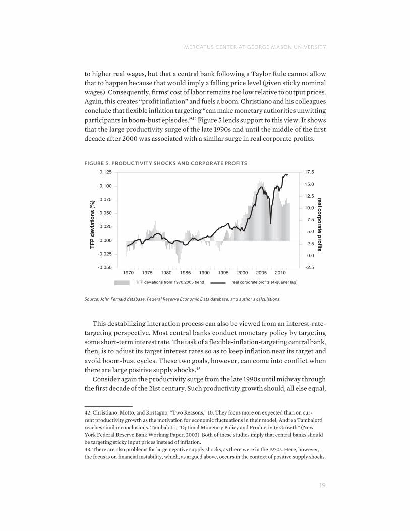
to higher real wages, but that a central bank following a Taylor Rule cannot allow that to happen because that would imply a falling price level (given sticky nominal wages). Consequently, firms’ cost of labor remains too low relative to output prices. Again, this creates “profit inflation” and fuels a boom. Christiano and his colleagues conclude that flexible inflation targeting “can make monetary authorities unwitting participants in boom-bust episodes.”42 Figure 5 lends support to this view. It shows that the large productivity surge of the late 1990s and until the middle of the first decade after 2000 was associated with a similar surge in real corporate profits.

FIGURE 5. PRODUCTIVITY SHOCKS AND CORPORATE PROFITS

Source: John Fernald database, Federal Reserve Economic Data database, and author’s calculations.

This destabilizing interaction process can also be viewed from an interest-rate-targeting perspective. Most central banks conduct monetary policy by targeting some short-term interest rate. The task of a flexible-inflation-targeting central bank, then, is to adjust its target interest rates so as to keep inflation near its target and avoid boom-bust cycles. These two goals, however, can come into conflict when there are large positive supply shocks.43

Consider again the productivity surge from the late 1990s until midway through the first decade of the 21st century. Such productivity growth should, all else equal,

42. Christiano, Motto, and Rostagno, “Two Reasons,” 10. They focus more on expected than on cur-rent productivity growth as the motivation for economic fluctuations in their model; Andrea Tambalotti reaches similar conclusions. Tambalotti, “Optimal Monetary Policy and Productivity Growth” (New York Federal Reserve Bank Working Paper, 2003). Both of these studies imply that central banks should be targeting sticky input prices instead of inflation.43. There are also problems for large negative supply shocks, as there were in the 1970s. Here, however, the focus is on financial instability, which, as argued above, occurs in the context of positive supply shocks.

Productivity Shocks and Corporate Profits

TFP deviations from 1970:2005 trend real corporate profits (4-quarter lag)

TFP

devi

atio

ns (%

)real corporate profits

1970 1975 1980 1985 1990 1995 2000 2005 2010-0.050

-0.025

0.000

0.025

0.050

0.075

0.100

0.125

-2.5

0.0

2.5

5.0

7.5

10.0

12.5

15.0

17.5


20

lead to an increase in the equilibrium or “natural” interest rate. The productivity gains, if permanent, will raise both the expected return on capital and the expected future income of households. The former will cause firms to invest more in facto-ries, machines, tools, and other capital. The latter will encourage households to increase their current consumption, either by saving less or by tapping into their higher future income via borrowing. These responses imply more borrowing and less saving by firms and households. These developments, in turn, will put upward pressure on interest rates. This is why the natural interest rate should, all else equal, go up.44

As noted above, the productivity gains will also create deflationary pressures that an inflation-targeting central bank will try to offset. To do that, the central bank will have to lower its target interest rate even though the natural interest rate is going up. Monetary authorities, therefore, will be pushing short-term interest rates below the stable, market-clearing level. To the extent this interest rate gap is expected to persist, long-term interest rates will also be pushed below their natural rate lev-el.45 These developments mean firms will see an inordinately low cost of capital, investors will see great arbitrage opportunities, and households will be incentivized to take on more debt. This opens the door for unwarranted capital accumulation, excessive reaching for yield, too much leverage, soaring asset prices, and ultimately a buildup of financial imbalances. By trying to promote price stability, then, the cen-tral bank will be fostering financial instability.46 These results have been formally shown by Eric Sims as well as by Lawrence Christiano and his coauthors to hold for a flexible inflation targeter following a Taylor Rule.47

44. Household time preferences and population growth also influence the natural interest rate. Here, I assume they are relatively constant and not important. These factors plus productivity growth make up the fundamentals that determine the natural interest rate. In the short run, though, there can also be cyclical determinants. These are spending shocks that create either positive or negative output gaps. Here, a positive (or negative) spending shock will lead to a temporarily higher (or lower) natural inter-est rate. For more on this, see Tom Bernhardsen and Karsten Gerdrup, “The Neutral Real Interest Rate,” Norges Bank Economic Bulletin 78, no. 2 (2007): 52–64. Also, technically, the natural growth rate will increase if the productivity growth rate increases. That appears to have been the case between the late 1990s and the middle of the first decade in the 21st century.45. Standard theory says long-term interest rates are an average of expected short-term interest rates over the same time frame plus a liquidity premium. Thus, if policymakers are expected to hold down short-term interest rates for an extended period of time, long-term interest will also be depressed.46. The discussion above is consistent with the Austrian view of business cycles. It also holds that pro-ductivity gains should be reflected in a falling price level and higher natural interest rates. When cen-tral banks do not allow these things to manifest, Austrians believe there will arise a “malinvestment,” or misallocation of capital spending, that eventually will lead to a bust. For more on the Austrian busi-ness cycle theory, see Roger Garrison, Time and Money: The Macroeconomics of Capital Structure (New York: Routledge Press, 2000); and Steven Horwitz, Microfoundations and Macroeconomics: An Austrian Perspective (New York: Routledge Press, 2009).47. Eric Sims, “Taylor Rules and Technology Shocks,” Economic Letters 116 (2012): 92–95; Lawrence Christiano, Cosmin L. Ilut, Roberto Motto, and Massimo Rostagno, “Monetary Policy and Stock Market Booms” (NBER Working Paper No. 16402, 2010).


21

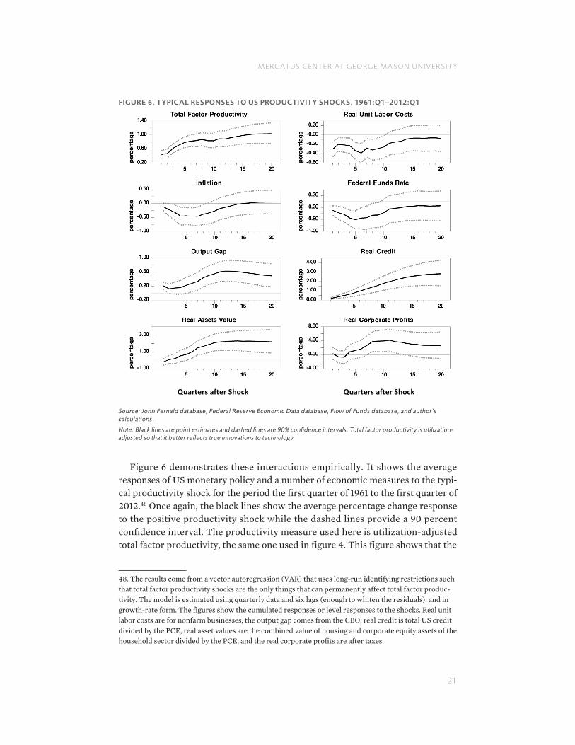
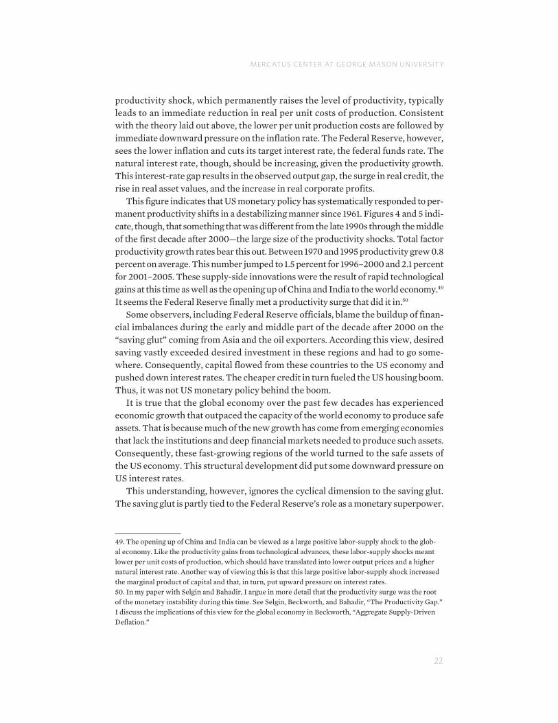
Figure 6 demonstrates these interactions empirically. It shows the average responses of US monetary policy and a number of economic measures to the typi-cal productivity shock for the period the first quarter of 1961 to the first quarter of 2012.48 Once again, the black lines show the average percentage change response to the positive productivity shock while the dashed lines provide a 90 percent confidence interval. The productivity measure used here is utilization-adjusted total factor productivity, the same one used in figure 4. This figure shows that the

48. The results come from a vector autoregression (VAR) that uses long-run identifying restrictions such that total factor productivity shocks are the only things that can permanently affect total factor produc-tivity. The model is estimated using quarterly data and six lags (enough to whiten the residuals), and in growth-rate form. The figures show the cumulated responses or level responses to the shocks. Real unit labor costs are for nonfarm businesses, the output gap comes from the CBO, real credit is total US credit divided by the PCE, real asset values are the combined value of housing and corporate equity assets of the household sector divided by the PCE, and the real corporate profits are after taxes.

Quarters after Shock Quarters after Shock

FIGURE 6. TYPICAL RESPONSES TO US PRODUCTIVITY SHOCKS, 1961:Q1–2012:Q1

Source: John Fernald database, Federal Reserve Economic Data database, Flow of Funds database, and author’s calculations.

Note: Black lines are point estimates and dashed lines are 90% confidence intervals. Total factor productivity is utilization-adjusted so that it better reflects true innovations to technology.


22

productivity shock, which permanently raises the level of productivity, typically leads to an immediate reduction in real per unit costs of production. Consistent with the theory laid out above, the lower per unit production costs are followed by immediate downward pressure on the inflation rate. The Federal Reserve, however, sees the lower inflation and cuts its target interest rate, the federal funds rate. The natural interest rate, though, should be increasing, given the productivity growth. This interest-rate gap results in the observed output gap, the surge in real credit, the rise in real asset values, and the increase in real corporate profits.

This figure indicates that US monetary policy has systematically responded to per-manent productivity shifts in a destabilizing manner since 1961. Figures 4 and 5 indi-cate, though, that something that was different from the late 1990s through the middle of the first decade after 2000—the large size of the productivity shocks. Total factor productivity growth rates bear this out. Between 1970 and 1995 productivity grew 0.8 percent on average. This number jumped to 1.5 percent for 1996–2000 and 2.1 percent for 2001–2005. These supply-side innovations were the result of rapid technological gains at this time as well as the opening up of China and India to the world economy.49 It seems the Federal Reserve finally met a productivity surge that did it in.50

Some observers, including Federal Reserve officials, blame the buildup of finan-cial imbalances during the early and middle part of the decade after 2000 on the “saving glut” coming from Asia and the oil exporters. According this view, desired saving vastly exceeded desired investment in these regions and had to go some-where. Consequently, capital flowed from these countries to the US economy and pushed down interest rates. The cheaper credit in turn fueled the US housing boom. Thus, it was not US monetary policy behind the boom.

It is true that the global economy over the past few decades has experienced economic growth that outpaced the capacity of the world economy to produce safe assets. That is because much of the new growth has come from emerging economies that lack the institutions and deep financial markets needed to produce such assets. Consequently, these fast-growing regions of the world turned to the safe assets of the US economy. This structural development did put some downward pressure on US interest rates.

This understanding, however, ignores the cyclical dimension to the saving glut. The saving glut is partly tied to the Federal Reserve’s role as a monetary superpower.

49. The opening up of China and India can be viewed as a large positive labor-supply shock to the glob-al economy. Like the productivity gains from technological advances, these labor-supply shocks meant lower per unit costs of production, which should have translated into lower output prices and a higher natural interest rate. Another way of viewing this is that this large positive labor-supply shock increased the marginal product of capital and that, in turn, put upward pressure on interest rates.50. In my paper with Selgin and Bahadir, I argue in more detail that the productivity surge was the root of the monetary instability during this time. See Selgin, Beckworth, and Bahadir, “The Productivity Gap.” I discuss the implications of this view for the global economy in Beckworth, “Aggregate Supply-Driven Deflation.”


23

The Federal Reserve holds the world’s main reserve currency, and many emerging markets are formally or informally pegged to dollar. Consequently, its monetary policy gets exported across the globe. This means that the other two monetary powers, the ECB and Japan, are mindful of US monetary policy lest their curren-cies become too expensive relative to the dollar and the other currencies pegged to the dollar. As a result, US monetary policy gets exported to some degree to Japan and the euro area as well. So when the Federal Reserve responded to the productivity surge by easing monetary policy, it forced the dollar-pegging coun-tries to buy up the new dollars it was creating in order to defend their pegs. These economies then used the dollars to buy up US debt. This increased the demand for safe assets. To the extent the ECB and the Bank of Japan also responded to US monetary policy, they too were acquiring foreign reserves and channeling credit back to the US economy. The easier US monetary policy became during this time, the greater the demand for US safe assets and the greater the amount of recycled credit coming back to the US economy.51

The saving glut, therefore, and its contribution to the buildup of financial imbal-ances at this time can be traced back in part to the interaction of inflation targeting with large positive supply shocks in the US economy. Inflation targeting and large positive supply shocks are simply a bad combination for financial stability.

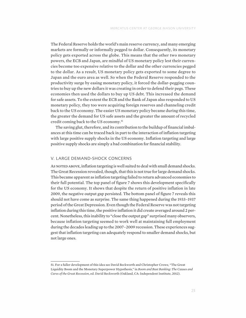
V. LARGE DEMAND-SHOCK CONCERNS

As noted above, inflation targeting is well suited to deal with small demand shocks. The Great Recession revealed, though, that this is not true for large demand shocks. This became apparent as inflation targeting failed to return advanced economies to their full potential. The top panel of figure 7 shows this development specifically for the US economy. It shows that despite the return of positive inflation in late 2009, the negative output gap persisted. The bottom panel of figure 7 reveals this should not have come as surprise. The same thing happened during the 1933–1937 period of the Great Depression. Even though the Federal Reserve was not targeting inflation during this time, the positive inflation it did create averaged around 2 per-cent. Nonetheless, this inability to “close the output gap” surprised many observers, because inflation targeting seemed to work well at maintaining full employment during the decades leading up to the 2007–2009 recession. These experiences sug-gest that inflation targeting can adequately respond to smaller demand shocks, but not large ones.

51. For a fuller development of this idea see David Beckworth and Christopher Crowe, “The Great Liquidity Boom and the Monetary Superpower Hypothesis,” in Boom and Bust Banking: The Causes and Cures of the Great Recession, ed. David Beckworth (Oakland, CA: Independent Institute, 2012).


24

FIGURE 7. INFLATION AND THE OUTPUT GAP

Source: Claudio Borio, Piti Disyatat, and Mikael Juselius, “Rethinking Potential Output: Embedding Information about the Financial Cycle” (BIS Working Paper No. 404, 2013); Robert Gordon and Robert Krenn, “The End of the Great Depression 1939–41: Fiscal Multipliers, Capacity Constraints, and Policy Contributions” (Northwestern University Working Paper, 2013); Federal Reserve Economic Data database; Flow of Funds database; author’s calculations.

Some inflation-targeting proponents argue that these output gaps could be closed under inflation targeting if central banks would only aim for a higher inflation rate.52 Other commentators, however, contend that it is not more inflation that is needed, but more demand. Moreover, behind this lack of demand is a more

52. Laurence Ball, “The Case for 4% Inflation,” Central Bank of the Republic of Turkey Central Bank Review, May 2013; Kenneth Rogoff, “Inflation is Still the Lesser Evil,” Project Syndicate, November 1, 2013, http://www.project-syndicate.org/commentary/the-benefits-of-higher-inflation-by-kenneth-rogoff.

Inflation and the Output GapUS Great Recession

inflation output gap

percentage

2007 2008 2009 2010 2011 2012 2013-5-4-3-2-101234

Inflation and the Output GapUS Great Depression

inflation output gap

percentage

1927 1929 1931 1933 1935 1937 1939 1941-40

-30

-20

-10

0

10

20

http://www.project-syndicate.org/commentary/the-benefits-of-higher-inflation-by-kenneth-rogoff


25

fundamental problem: excess money demand.53 This problem occurs when desired money balances exceed actual money holdings and, in turn, cause individuals and firms to rebalance their portfolios away from risky assets toward safe, liquid ones. Collectively, this rebalancing lowers asset prices, increases risk premiums, and ultimately reduces aggregate spending. Excess money demand, these commenta-tors argue, is the real culprit behind the persistent output gap. Inflation targeting’s inability, then, to restore full employment is because it has not been able to solve the problem of large excess money demand during this time.

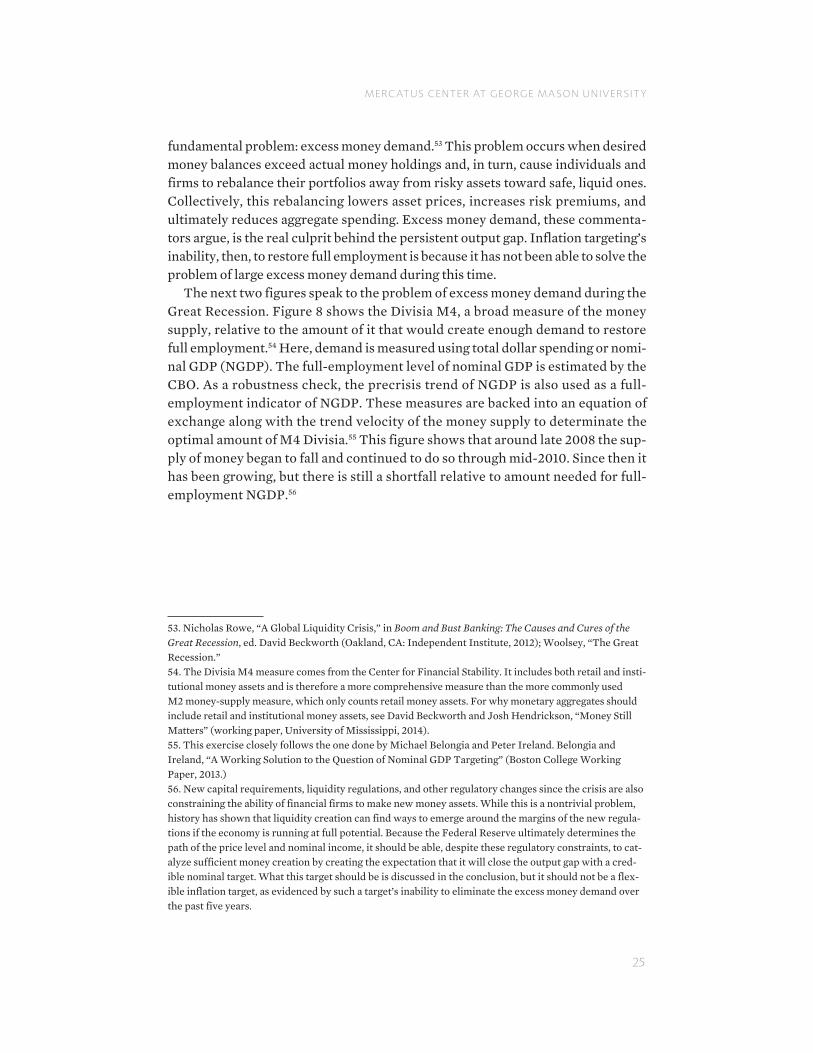
The next two figures speak to the problem of excess money demand during the Great Recession. Figure 8 shows the Divisia M4, a broad measure of the money supply, relative to the amount of it that would create enough demand to restore full employment.54 Here, demand is measured using total dollar spending or nomi-nal GDP (NGDP). The full-employment level of nominal GDP is estimated by the CBO. As a robustness check, the precrisis trend of NGDP is also used as a full-employment indicator of NGDP. These measures are backed into an equation of exchange along with the trend velocity of the money supply to determinate the optimal amount of M4 Divisia.55 This figure shows that around late 2008 the sup-ply of money began to fall and continued to do so through mid-2010. Since then it has been growing, but there is still a shortfall relative to amount needed for full-employment NGDP.56

53. Nicholas Rowe, “A Global Liquidity Crisis,” in Boom and Bust Banking: The Causes and Cures of the Great Recession, ed. David Beckworth (Oakland, CA: Independent Institute, 2012); Woolsey, “The Great Recession.”54. The Divisia M4 measure comes from the Center for Financial Stability. It includes both retail and insti-tutional money assets and is therefore a more comprehensive measure than the more commonly used M2 money-supply measure, which only counts retail money assets. For why monetary aggregates should include retail and institutional money assets, see David Beckworth and Josh Hendrickson, “Money Still Matters” (working paper, University of Mississippi, 2014).55. This exercise closely follows the one done by Michael Belongia and Peter Ireland. Belongia and Ireland, “A Working Solution to the Question of Nominal GDP Targeting” (Boston College Working Paper, 2013.)56. New capital requirements, liquidity regulations, and other regulatory changes since the crisis are also constraining the ability of financial firms to make new money assets. While this is a nontrivial problem, history has shown that liquidity creation can find ways to emerge around the margins of the new regula-tions if the economy is running at full potential. Because the Federal Reserve ultimately determines the path of the price level and nominal income, it should be able, despite these regulatory constraints, to cat-alyze sufficient money creation by creating the expectation that it will close the output gap with a cred-ible nominal target. What this target should be is discussed in the conclusion, but it should not be a flex-ible inflation target, as evidenced by such a target’s inability to eliminate the excess money demand over the past five years.


26

FIGURE 8. BROAD MONEY SUPPLY

Source: Center for Financial Stability, Federal Reserve Economic Data database, and author’s calculations.

Figure 9 plots the output gap against the percent of household assets that are highly liquid.57 The higher this ratio is, the greater the demand for money-like assets and vice versa. This ratio rose sharply in 2008 during the Great Recession, as eco-nomic uncertainty drove households to safe, more liquid assets. Though this ratio has started to come down, it is still highly elevated. Presumably, this is because of the dribble of bad economic news like the ongoing eurozone crisis, the multiple fis-cal showdowns in Washington, DC, and concerns of a China slowdown. The output gap is almost the mirror opposite of this elevated demand for money-like assets. The R2 between these two measures is 67 percent. The easiest interpretation of this figure is that this high money demand is behind the slump.

Ironically, this elevated demand for liquidity is why there has been a shortfall of money assets. By holding on to an inordinately high level of liquid assets, households are not only spending less themselves, but they are also causing firms to spend less. This means there is less demand for financial intermediation by households and firms. Similarly, financial firms in this economic environment are less willing to issue credit. Most money, however, is created by financial firms issuing liabilities. For example, a bank making a loan implies the creation of new deposits or money in the borrower’s checking account. Thus, even as households desire more liquid assets, their actions in doing this lead to fewer money assets. This shortfall of money relative to the demand for it implies there is still a problem of excess money demand.

57. Household liquid assets include cash, checking and saving accounts, time deposits, money-market mutual funds, treasury securities, and agency securities.


27

Inflation targeting has not been able to solve it. Here, too, inflation targeting has seemed to reach its limits.

VI. JUDGMENT-CALL CONCERNS

When inflation targeting was first introduced by New Zealand and Canada, the sole objective was price stability. As noted above, though, this program gradually evolved into flexible inflation targeting. Proponents of inflation targeting saw this as a positive development. Bernanke, for example, noted it gave central banks more ability to tame the business cycle:

The adoption of this approach helped central banks anchor longer-term inflation expectations, which in turn increased the effective scope of monetary policy to stabilize output and employment in the short run.58

Like many others, he saw this “constrained discretion” as an essential part of con-ducting good monetary policy. It requires, though, that policymakers know how best to use it. In particular, monetary authorities must be capable of discerning between

58. Ben Bernanke, “The Effects of the Great Recession.”

FIGURE 9. ELEVATION OF LIQUIDITY DEMAND

Source: Claudio Borio, Piti Disyatat, and Mikael Juselius, “Rethinking Potential Output: Embedding Information about the Financial Cycle” (BIS Working Paper No. 404, 2013); Federal Reserve Economic Data database; and author’s calculations.

Note: Household liquid assets include cash, checking and savings accounts, time deposits, money-market mutual funds, treasury securities, and agency securities. The output gap comes from Borio, Disyetat, and Juselius’s 2013 BIS working paper.

Elevated Liquidity Demand

output gaphousehold sector: liquid assets as a % of total assets

outp

ut g

ap (%

)liquidity dem

and (%)

1999 2001 2003 2005 2007 2009 2011 2013-5

-4

-3

-2

-1

0

1

2

3

4

9.0

9.5

10.0

10.5

11.0

11.5

12.0

12.5

13.0

13.5


28

demand and supply shocks in real time, because monetary policy can only produc-tively respond to the former. This is often difficult, if not impossible, and therefore requires judgment calls. Lars Svensonn notes, for example, that this is the case when dealing with concerns about wide swings in asset-price bubbles. He acknowledges this is “an area where good judgment is crucial.”59

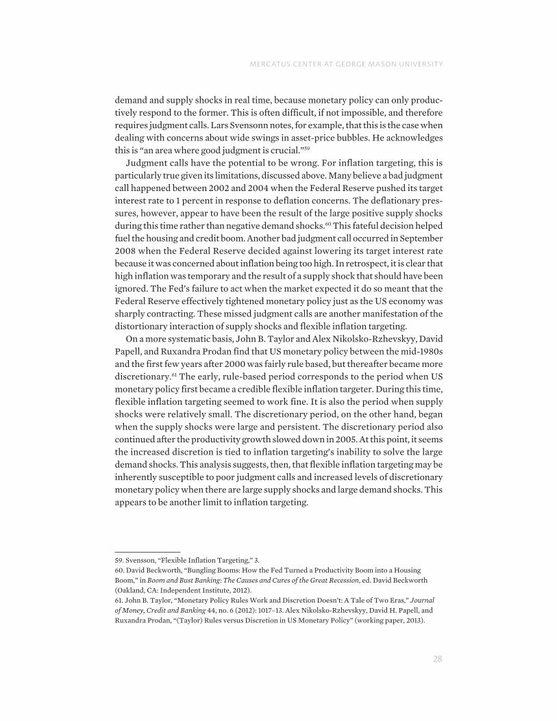
Judgment calls have the potential to be wrong. For inflation targeting, this is particularly true given its limitations, discussed above. Many believe a bad judgment call happened between 2002 and 2004 when the Federal Reserve pushed its target interest rate to 1 percent in response to deflation concerns. The deflationary pres-sures, however, appear to have been the result of the large positive supply shocks during this time rather than negative demand shocks.60 This fateful decision helped fuel the housing and credit boom. Another bad judgment call occurred in September 2008 when the Federal Reserve decided against lowering its target interest rate because it was concerned about inflation being too high. In retrospect, it is clear that high inflation was temporary and the result of a supply shock that should have been ignored. The Fed’s failure to act when the market expected it do so meant that the Federal Reserve effectively tightened monetary policy just as the US economy was sharply contracting. These missed judgment calls are another manifestation of the distortionary interaction of supply shocks and flexible inflation targeting.

On a more systematic basis, John B. Taylor and Alex Nikolsko-Rzhevskyy, David Papell, and Ruxandra Prodan find that US monetary policy between the mid-1980s and the first few years after 2000 was fairly rule based, but thereafter became more discretionary.61 The early, rule-based period corresponds to the period when US monetary policy first became a credible flexible inflation targeter. During this time, flexible inflation targeting seemed to work fine. It is also the period when supply shocks were relatively small. The discretionary period, on the other hand, began when the supply shocks were large and persistent. The discretionary period also continued after the productivity growth slowed down in 2005. At this point, it seems the increased discretion is tied to inflation targeting’s inability to solve the large demand shocks. This analysis suggests, then, that flexible inflation targeting may be inherently susceptible to poor judgment calls and increased levels of discretionary monetary policy when there are large supply shocks and large demand shocks. This appears to be another limit to inflation targeting.

59. Svensson, “Flexible Inflation Targeting,” 3. 60. David Beckworth, “Bungling Booms: How the Fed Turned a Productivity Boom into a Housing Boom,” in Boom and Bust Banking: The Causes and Cures of the Great Recession, ed. David Beckworth (Oakland, CA: Independent Institute, 2012).61. John B. Taylor, “Monetary Policy Rules Work and Discretion Doesn’t: A Tale of Two Eras,” Journal of Money, Credit and Banking 44, no. 6 (2012): 1017–13. Alex Nikolsko-Rzhevskyy, David H. Papell, and Ruxandra Prodan, “(Taylor) Rules versus Discretion in US Monetary Policy” (working paper, 2013).


29

VII. POLICY IMPLICATIONS

The above study raises a number of concerns about the limits of inflation targeting. Its success depends on supply shocks being few and demand shocks being small. While these conditions prevailed for several decades and allowed inflation targeting to become a credible nominal anchor, that run of good luck ended in the late 1990s. Inflation targeting, in other words, is a monetary-policy regime that is not robust enough to handle the changing structure of the US economy.

What, then, would characterize a robust monetary-policy regime? Based on the discussion above, it would be one that does not respond to supply shocks, but does vigorously respond to demand shocks. The problem with an inflation-targeting cen-tral bank is that it has a hard time ignoring supply shocks because they move infla-tion. The central bank should only respond to inflation caused by demand shocks, but it is hard to distinguish the source of inflation movements in real time. One way to get around this problem is to directly target demand itself. That is, the Federal Reserve could aim to stabilize the growth of total dollar spending. This way the Federal Reserve would not have to worry about divining the sources of movements in inflation.

This understanding can be illustrated by recalling how businesses best handle positive productivity shocks. As noted earlier, productivity gains mean lower per unit production costs for firms that, in turn, should translate into lower output prices given competitive pressures. Here, the increase in a firm’s output from the productivity gains is matched by a decrease in its sales price. For an economy-wide productivity innovation that affects many firms, this response would manifest itself in rising real GDP growth alongside a declining price level. For the same reasons, an economy-wide negative productivity shock would lead to falling real GDP and a rising price level.

Note that the price level times real GDP is equal to total dollar spending. That is, the dollar price of everything produced and sold equals, by definition, the total number of times money is spent. This relationship implies, then, that if the Federal Reserve directly targeted the growth of total dollar spending it would by default be allowing the price level to move inversely with productivity-driven changes in real GDP.62 This would amount to a monetary-policy regime that ignores supply shocks.

62. This relationship can be summarized by the following equation:M × V = P × Y.

This is the famous equation of exchange where M = money; V = number of times money is spent, or the “velocity” of money; P = the price level; and Y = real GDP. In the case of a positive productivity shock, the price level would be falling and real GDP increasing, making the right-hand side of the equation relatively stable. This would imply that the left-hand side, which shows total dollar spending, would be relatively stable too. Most proponents of this approach envision some positive growth rate for total dol-lar spending. Consequently, whether there was outright deflation or just disinflation would depend on the targeted growth rate for M × V.


30

To be clear, ignoring supply shocks means allowing such shocks to be reflected in relative price changes. No attempt is made to offset them or their effect on the price level.63 Ignoring supply shocks also means allowing market interest rates to more closely track the market-clearing or natural-interest-rate level. Doing so reduces financial instability.

To see this, recall that a positive productivity shock pushes up the natural interest rate. A central bank that targeted the growth of total dollar spending would have to raise its interest-rate target to keep spending stable. This is because the higher pro-ductivity growth would raise expected profitability for firms and expected income for households, and thus encourage them to spend more. Raising the interest-rate target to its new natural rate level would ensure their spending did not get too exces-sive. An inflation-targeting central bank, on the other hand, would be tempted to lower its interest-rate target because of the disinflationary pressures created by the productivity shock. This is, arguably, what the Federal Reserve did between 2002 and 2004. As discussed earlier, pushing market interest rates below their natural-interest-rate level will lead to unwarranted capital accumulation, excessive reach-ing for yield, too much leverage, soaring asset prices, and a buildup of financial imbalances. A total-dollar-spending target would avoid this temptation because it would focus on stabilizing expenditures, not the price level. It therefore would bet-ter promote financial stability.

This approach could also solve the problem that inflation targeting has with large demand shocks. It would require that monetary policy target the growth path of total dollar spending. This would commit monetary authorities to make up for past misses both above and below the target so that the targeted growth path would be maintained. This is illustrated in the top panel of figure 10. It shows a scenario where monetary policy is targeting 4 percent growth—the slope of the line—in total dollar spending. Now imagine some adverse economic development causes expenditures to fall in year Y1. The Federal Reserve would make up for the miss the next year, Y2, by increasing total dollar spending faster than 4 percent—the steeper slope—until it has caught up to its target path (the gray line). A similar response would follow a spending boom that pushed expenditures above the targeted path, as seen in the bottom panel of figure 10. An inflation target has a hard time doing this because it targets a growth rate instead of a growth path. An inflation target, in other words, cannot do catch-up or slow-down growth to some trend because that would require moving inflation away from its target.64

63. See the “Productivity and Relative Prices” chapter in George Selgin’s Less than Zero for more on this point.64. If the central bank adopted a growth-path target for the price level it would avoid this problem. However, this would face the same challenges with supply shocks as an inflation target would.


31

FIGURE 10. A GROWTH-PATH TARGET

A growth-path target for total dollar spending has two other attractive features. First, it would minimize the likelihood of large demand shocks emerging in the first place. If households and firms anticipated that the Federal Reserve would do what-ever is necessary to return total dollar spending to its targeted path, then they would be less likely to cut back on spending and increase their holding of liquid assets in


32

the first place. Large demand shocks, consequently, should become less common. Second, the Federal Reserve would become much more predictable, as the targeted growth path would put a constraint on monetary policy. That would mean fewer judgment calls by monetary authorities.

In summary, targeting the growth path of total dollar spending would improve financial stability, minimize large demand shocks, and reduce the number of judg-ment calls by monetary authorities—the very problems that plague inflation tar-geting.65 For these reasons, an increasing number of observers have called for its adoption by the Federal Reserve.66

VIII. CONCLUSION

This paper has shown that inflation targeting has limits. It is not robust to eco-nomic environments where there are many supply and large demand shocks. It also seems to contribute to financial instability. Though it ably served as a nominal anchor for several decades, its success appears to have been dependent on the benign eco-nomic environment of that time. In short, inflation targeting got lucky. With the global economy becoming more financially developed and integrated, these prob-lems with inflation targeting are only likely to grow. Consequently, this paper argues the Federal Reserve should now target the growth path of total dollar spending.

Inflation targeting’s time has come and gone. It is now time to retarget mon-etary policy.

65. Note that this approach is also consistent with Austrian economics because it would allow deflation in response to productivity gains and would better keep market interest rates in line with their natural rate level. The Selgin version of this rule would be the most Austrian version. See Selgin, Less than Zero.66. See, for example, Selgin, Less than Zero; Sumner, “Retargeting the Fed”; Sumner, “The Case for Nominal GDP Targeting” (Mercatus Research, Mercatus Center at George Mason University, Arlington, VA, October 23, 2012), http://mercatus.org/sites/default/files/NGDP_Sumner_v-10-copy.pdf; Jeffrey Frankel, “The Death of Inflation Targeting”; David Beckworth and Ramesh Ponnuru, “Monetary Regime Change: An Old Order Fails,” National Review, June 11, 2012, 33–35; and Michael Woodford, “Methods of Policy Accommodation at Interest Rate Lower Bound,” (speech, Jackson Hole Symposium, Kansas City Federal Reserve Bank, Kansas City, August 31, 2012). The more common name for this approach is nomi-nal GDP level targeting.

http://mercatus.org/sites/default/files/NGDP_Sumner_v-10-copy.pdf