Embed Size (px)
Citation preview

ZMP-HH/10-18Hamburger Beitrage zur Mathematik 387
[1008.0082 [hep-th]]
A modular invariant bulk theoryfor the c = 0 triplet model
Matthias R. Gaberdiela∗, Ingo Runkelb† and Simon Wooda‡
a Institute for Theoretical Physics, ETH Zurich8093 Zurich, Switzerland
b Department Mathematik, Universitat HamburgBundesstraße 55, 20146 Hamburg, Germany
July 2010
Abstract
A proposal for the bulk space of the logarithmicW2,3-triplet model at central charge zerois made. The construction is based on the idea that one may reconstruct the bulk theoryof a rational conformal field theory from its boundary theory. The resulting bulk space isa quotient of the direct sum of projective representations, which is isomorphic, as a vectorspace, to the direct sum of tensor products of the irreducible representations with theirprojective covers. As a consistency check of our analysis we show that the partition functionof the bulk theory is modular invariant, and that the boundary state analysis is compatiblewith the proposed annulus partition functions of this model.
∗Email: [email protected]†Email: [email protected]‡Email: [email protected]

Contents
1 Introduction and summary 31.1 The chiral W2,3-model . . . . . . . . . . . . . . . . . . . . . . . . . . . . . . . . . 41.2 The boundary theory . . . . . . . . . . . . . . . . . . . . . . . . . . . . . . . . . . 51.3 From boundary to bulk . . . . . . . . . . . . . . . . . . . . . . . . . . . . . . . . . 71.4 The boundary states . . . . . . . . . . . . . . . . . . . . . . . . . . . . . . . . . . 9
2 The construction of the bulk space 112.1 From boundary to bulk — the original construction . . . . . . . . . . . . . . . . . 11
2.1.1 The algebra of boundary fields . . . . . . . . . . . . . . . . . . . . . . . . . 122.1.2 Bulk-boundary maps . . . . . . . . . . . . . . . . . . . . . . . . . . . . . . 122.1.3 Characterising the bulk space . . . . . . . . . . . . . . . . . . . . . . . . . 14
2.2 The proposal for the bulk space of the W2,3-model . . . . . . . . . . . . . . . . . . 142.2.1 Characterising the terminal object . . . . . . . . . . . . . . . . . . . . . . 152.2.2 Projective covers . . . . . . . . . . . . . . . . . . . . . . . . . . . . . . . . 162.2.3 Computing the Kernel . . . . . . . . . . . . . . . . . . . . . . . . . . . . . 17
2.3 Properties of the resulting bulk space . . . . . . . . . . . . . . . . . . . . . . . . . 182.3.1 The edge of the Kac table . . . . . . . . . . . . . . . . . . . . . . . . . . . 182.3.2 The interior of the Kac table . . . . . . . . . . . . . . . . . . . . . . . . . . 192.3.3 Consistency conditions . . . . . . . . . . . . . . . . . . . . . . . . . . . . . 19
3 The boundary state analysis 203.1 Reconstructing the boundary states . . . . . . . . . . . . . . . . . . . . . . . . . . 203.2 The Ishibashi states . . . . . . . . . . . . . . . . . . . . . . . . . . . . . . . . . . . 21
3.2.1 The edge of the Kac table . . . . . . . . . . . . . . . . . . . . . . . . . . . 223.2.2 The interior of the Kac table . . . . . . . . . . . . . . . . . . . . . . . . . . 22
3.3 Overlaps of Ishibashi states . . . . . . . . . . . . . . . . . . . . . . . . . . . . . . 243.3.1 The corner of the Kac table . . . . . . . . . . . . . . . . . . . . . . . . . . 253.3.2 The edge of the Kac table . . . . . . . . . . . . . . . . . . . . . . . . . . . 253.3.3 The interior of the Kac table . . . . . . . . . . . . . . . . . . . . . . . . . . 27
4 Conclusion 31
A W2,3-representations 32A.1 Composition series . . . . . . . . . . . . . . . . . . . . . . . . . . . . . . . . . . . 32A.2 Modular transformations . . . . . . . . . . . . . . . . . . . . . . . . . . . . . . . . 35
B Projective cover of W(0) 36B.1 Fusion rules . . . . . . . . . . . . . . . . . . . . . . . . . . . . . . . . . . . . . . . 36B.2 Composition series . . . . . . . . . . . . . . . . . . . . . . . . . . . . . . . . . . . 39
2

1 Introduction and summary
Logarithmic conformal field theories [1] with c = 0 appear quite generically in models with a non-trivial fixed point theory but a trivial generating function [2]. Prime examples of such theoriesare systems with quenched disorder [3] that include, among others, percolation [4, 5, 6, 7, 8, 9, 10]and polymers [11, 12, 13, 14]. Another area where c = 0 conformal field theories have recentlymade an appearance is as the dual theory for chiral gravity in AdS3 [15], and also in this contextthere are indications that the conformal field theory is logarithmic [16, 17].
Much has been learned over the last fifteen years about logarithmic conformal field theories. Inparticular, the triplet theory at c = −2 [18] has been understood in great detail [19, 20, 21, 22], ashave been the WZW models with supergroup target spaces [23, 24, 25, 26, 27, 28]. There has alsobeen some progress towards understanding WZW models at fractional level that show logarithmicbehaviour [29, 30, 31, 32], logarithmic extensions of minimal models [33], and the structure ofgeneral indecomposable Virasoro-representations [34]. However, most of the models that havebeen understood behave quite differently from the theory at c = 0. Indeed, c = 0 is special sincethe Virasoro field is ‘null’ at c = 0 in the sense that it has a vanishing 2-point function. Asa consequence the vacuum representation of the chiral algebra is not irreducible, and a numberof novel phenomena appear. Many of these are also shared by the whole family of logarithmicminimal Wp,q-models with p, q ≥ 2 [35] that have attracted a lot of attention during the last fouryears [36, 37, 38, 9, 39, 40, 41, 42, 43, 44, 45, 46]. Significant progress has been made for thesetheories, and the fusion rules as well as the modular properties of the chiral representations arenow fairly well understood. In [41] a consistent boundary theory was proposed for the simplestmember of this family of models, the theory with c2,3 = 0, and the generalisation to all Wp,q-models was sketched in [43]. However, so far an understanding of the corresponding bulk theoryis missing.
In this paper we shall construct the bulk space of states for the W2,3-model that correspondsto the boundary theory of [41]. Our strategy is to reconstruct the bulk theory, starting fromthe boundary ansatz. This idea goes back to [47, 48, 49] (see also [50] and [51, 52]), and wassuccessfully applied to the logarithmic W1,p triplet models (and in particular to the theory atc = −2) in [53]. There are a number of subtleties that arise in the present context, and as aconsequence the analysis is technically considerably harder than in [53]. However, the resultingspace of bulk states still has all properties one should expect it to have. In particular, the partitionfunction is modular invariant, and it allows for the construction of boundary states in agreementwith the prediction of [41]. Both of these are non-trivial consistency checks, and we are thereforeconfident that our bulk ansatz defines a consistent bulk conformal field theory.
Many structural features are similar to what happens for the W1,p-models (and in particularat c = −2). For example the space Hbulk of bulk states is of the form
Hbulk =⊕
i∈IrrW(i)⊗C P(i) as (Ldiag0 , Ldiag
0 )- graded vector space , (1.1)
where the sum runs over all irreducible W2,3-representations W(i), P(i) denotes the projective
cover of W(i), and Ldiag0 (resp. Ldiag
0 ) refers to the diagonal part of the action of L0 (resp. L0).However, there are also a number of remarkable new phenomena that appear for the W2,3-modelat c = 0. Firstly, in distinction to all rational CFTs and the W1,p-models, the bulk theorydoes not contain W2,3 ⊗C W2,3 as a sub-representation, but only as a sub-quotient. The second
3

surprising feature is that in order to reproduce the annulus amplitudes one only needs ten Ishibashistates, while the characters of the representations labelling the boundary states of [41] span a 12-dimensional space. The actual boundary states must involve additional Ishibashi states in orderfor the bulk-boundary correlators to be non-degenerate in the bulk entry, but these additionalIshibashi states do not contribute to the annulus diagrams (without any additional insertions),and are hence invisible from the point of view of the usual annulus analysis.
The paper is organised as follows. In the remainder of this introduction we shall first reviewsome of the results from [41] that we shall need in the rest of the paper. In particular, Section 1.1reviews the representation theory of theW2,3-algebra in question, while Section 1.2 summarises theboundary theory that was proposed in [41]. In Section 1.3 we sketch the general strategy for theconstruction of the bulk theory starting from this boundary ansatz. Finally, Section 1.4 describesthe main features of the corresponding boundary state analysis. These sections are meant to give anon-technical account of these considerations; the actual details are then spelled out in Sections 2and 3, respectively, while Section 4 contains our conclusions. Some of the tables, diagrams andtechnical constructions have been delegated into appendices.
1.1 The chiral W2,3-model
The Wp,q-models have central charge
cp,q = 1− 6(p− q)2
pq, (1.2)
where p and q are a pair of positive coprime integers. In the following we shall only consider thecase (p, q) = (2, 3) for which c2,3 = 0. The chiral algebra W ≡ W2,3 is generated by the Virasoroalgebra, as well as by a triplet of fields of conformal weight h = 15. In the vacuum representationL−1Ω = 0, but T = L−2Ω 6= 0. Since the positive modes annihilate T (in particular, c = 0implies that L2T = 0), the vacuum representation contains a proper subrepresentation, namelythe highest weight representation W(2) generated from T by the action of the negative modes.Thus W is not irreducible, but has the schematic structure
Ω // ((× T W(2) //
h = 0 h = 1 h = 2
(1.3)
The irreducible representations of the W algebra are described by the finite Kac table [35]
s = 1 s = 2 s = 3
r = 1 0, 2, 7 0, 1, 5 13, 10
3
r = 2 58, 33
818, 21
8−124, 35
24
(1.4)
Here each entry h is the conformal dimension of the highest weight states of an irreducible rep-resentation, which we shall denote by W(h). There is only one representation corresponding to
4

h = 0, namely the one-dimensional vacuum representation W(0), spanned by the vacuum vectorΩ. The significance of the grey boxes will be explained below in Section 1.2.
As is familiar from other logarithmic theories, the 13 irreducible representations in (1.4) donot close among themselves under fusion. The minimal set of representations which includes(1.4) and is closed under fusion and taking conjugates involves in addition the 22 indecomposablerepresentations
W , W∗ , Q , Q∗ , R(2)(0, 2)7 , R(2)(2, 7) , R(2)(0, 1)5 , R(2)(1, 5) ,
R(2)(0, 2)5 , R(2)(2, 5) , R(2)(0, 1)7 , R(2)(1, 7) , R(2)(13, 1
3) ,
R(2)(13, 10
3) , R(2)(5
8, 5
8) , R(2)(5
8, 21
8) , R(2)(1
8, 1
8) , R(2)(1
8, 33
8) ,
R(3)(0, 0, 1, 1) , R(3)(0, 0, 2, 2) , R(3)(0, 1, 2, 5) , R(3)(0, 1, 2, 7) ,
(1.5)
whose structure (including characters and embedding diagrams) are described in some detail in [41,App. A] and Appendix A below. Note that in addition to the chiral algebra W also its conjugaterepresentation W∗ appears; because of the structure of (1.3) it is not isomorphic to W . (Indeed,the embedding structure of W∗ can be obtained from that of W by reversing the direction of thearrow Ω→ T .)
The associative fusion rules of all of these 13 + 22 = 35 representations were given explicitly in[41]. They were derived based on a direct calculation of the fusion rules for the Virasoro subalgebra(compare [36]), and agree with what was obtained based on a lattice analysis in [9, 40].
For the construction of the bulk theory the projective covers of the irreducible representationsplay an important role. Let us denote the projective cover of the representation W(h) by P(h).Then we have the identifications (this was already suggested in [41])
P(1) = R(3)(0, 0, 1, 1) , P(2) = R(3)(0, 0, 2, 2) , P(5) = R(3)(0, 1, 2, 5) ,
P(7) = R(3)(0, 1, 2, 7) , P(13) = R(2)(1
3, 1
3) , P(10
3) = R(2)(1
3, 10
3) ,
P(58) = R(2)(5
8, 5
8) , P(21
8) = R(2)(5
8, 21
8) , P(1
8) = R(2)(1
8, 1
8) ,
P(338
) = R(2)(18, 33
8) , P(−1
24) =W(−1
24) , P(35
24) =W(35
24) .
(1.6)
As was also explained in [41], none of the representations in (1.4) and (1.5) can be the projectivecover of W(0). On the other hand, on general grounds [54, 55, 56] one may expect that everyirreducible representation has a projective cover. We shall propose the structure of the projectivecover P(0) forW(0) in Section 2.2.2 below. In Appendix B we shall derive some further propertiesof P(0), and deduce its fusion rules with most of the representations in (1.4) and (1.5).
1.2 The boundary theory
For non-logarithmic rational conformal field theories with charge-conjugation modular invariant(the ‘Cardy case’) the boundary conditions that preserve the chiral symmetry are in one-to-onecorrespondence to the representations of the chiral algebra [57]. The situation is similar for theW1,p-models, but as was explained in [41], the situation is more complicated for the W2,3-modelat c = 0. Indeed, consistent boundary conditions can only be associated to a subset of the 35
5

representations above, namely to those 26 representations that are not in grey boxes.1 Theseallowed representations are characterised by the property that the conjugate representation agreeswith the dual representation. This condition guarantees that the space of boundary fields has anon-degenerate bilinear pairing, i.e. that the boundary 2-point functions are non-degenerate (formore details see [41]). In particular, this then also implies that the space of boundary fields ofany consistent boundary condition cannot just be W2,3 itself.
The space of open string states HR→S between two boundary conditions labelled by R andS is given by the fusion product HR→S = S ⊗f R∗, where ⊗f denotes the fusion product ofW-representations and R∗ is the conjugate representation to R; this is as in the usual Cardy case.
A convenient tool to analyse the annulus partition functions, i.e. the characters of the W-representation HR→S , is provided by the (additive) Grothendieck group K0. It consists of equiva-lence classes [R] of representations R, where two representations R and R′ are equivalent iff theyhave the same character2, χR(q) = χR′(q). Thus, giving the element [R] in K0 for a representationR is the same as specifying its character, and we can describe the annulus partition functions aselements [HR→S ] ∈ K0.
The additive group K0 is generated by 13 elements, corresponding to the characters of theirreducible representations. The representations which lead to consistent boundary conditions,i.e. those not in grey boxes, generate a subgroup Kb
0 of K0 spanned (for example) by the following12 independent elements [41, Sect. 2.4],
Kb0 = spanZ
([W(h)]
∣∣h = 0, 13, 10
3, 5
8, 33
8, 1
8, 21
8, −1
24, 35
24
)⊕ 2Z
([W(2)]+[W(7)]) ⊕ 2Z
([W(1)]+[W(5)]) ⊕ 2Z
([W(2)]+[W(5)]) .
(1.7)
The fusion product makes Kb0 (but not K0) into a ring. By definition, this means that the annulus
partition function for boundary conditions R and S can be written as
[HR→S ] = [S] · [R∗] . (1.8)
Clearly, two representations R and R′ lead to the same annulus partition function [HR→S ] =[HR′→S ] if they have the same character, because then [R] = [R′]. However, the converse is nottrue: the ring Kb
0 contains a 2-dimensional null ideal spanned by
N1 = [W(58)]− [W(33
8)]− [W(1
8)] + [W(21
8)]− [W(−1
24)] + [W(35
24)] , N2 = [W(0)] . (1.9)
These two elements have the property that N1 · C = 0 = N2 · C for all C ∈ Kb0. Thus any two
representationsR andR′ with the property that [R]−[R′] ∈ spanZ([N1], [N2]
)also lead to identical
annulus partition functions. For example, the two representations R = W(58) ⊕W(21
8) ⊕W(35
24)
and R′ = W(338
) ⊕W(18) ⊕W(−1
24) have the property that [R] − [R′] = [N1]. As a consequence
their annulus amplitudes with any boundary condition S agrees, [HR→S ] = [HR′→S ]. This doesnot imply that R and R′ have identical boundary states ‖R〉〉 and ‖R′〉〉; indeed, one may expectthat suitable correlators of bulk fields on a disc can distinguish two boundary conditions R andR′ whenever [R] 6= [R′] in Kb
0. However, it does mean that 10 Ishibashi states are sufficient toreproduce all annulus partition functions as overlaps 〈〈R‖qL0 qL0‖S〉〉.
1There may, however, be additional boundary conditions associated to other classes of representations.2This description of K0 is correct if the irreducible representations of W have linearly independent characters,
which is the case for W2,3.
6

1.3 From boundary to bulk
For non-logarithmic rational conformal field theories one can reconstruct the bulk theory from oneconsistent boundary condition [48, 49]. The same method was also successfully applied in [53] tothe case of the logarithmic W1,p-models. The idea behind the construction is as follows.
Suppose we are given a boundary condition together with its space of boundary fields andthe associated operator product expansion (OPE). We consider the disc correlator involving oneboundary field and one field from the yet-to-be-constructed space of bulk states. This correlatordefines a pairing between the bulk and boundary degrees of freedom
H(ans)bulk ×Hbnd → C : (ψ, φ) 7→
⟨V (ψ, 0)V (φ, u)
⟩disc
, (1.10)
where |u| = 1 is a point on the perimeter of the disc, and the index ‘(ans)’ indicates that at thisstage we can only make an ansatz for the bulk space of states. If φ ∈ R⊗C S is in a representationof the left- and right-moving chiral algebra, then the map (1.10) is uniquely determined up to someconstants (one for each allowed fusion channel) since, by the usual doubling trick, the correlatorcan be thought of as a chiral 3-point function. These constants encode the bulk-boundary OPE,and they are constrained by two necessary requirements. First of all, it follows from generalprinciples (non-degeneracy of the bulk 2-point function on the sphere) that the map (1.10) has tobe non-degenerate in the first (bulk) entry. Furthermore, given the OPE of the boundary fields,it also defines correlators involving more than one boundary field, and these have to satisfy theappropriate locality conditions, see Section 2.1.2. The ‘correct’ space of bulk states is then simplythe largest possible space compatible with these requirements. It was proven in [51, 52] that in thenon-logarithmic setting, this construction reproduces indeed the unique space of bulk states that iscompatible with the given boundary condition. For the logarithmic W1,p-models the constructionwas also shown to lead to sensible results; in particular, the known c = −2 bulk theory of [20] wascorrectly reproduced by this method in [53].
In all of these constructions the analysis is simplest if the space of boundary fields just consistsof the chiral algebra (or VOA) itself. This is the case for the ‘identity Cardy brane’ and it leadsto the charge-conjugation modular invariant theory. Indeed, such a brane exists for all the W1,p-models, and it was taken as the starting point for the analysis of [53]. As already noted at thebeginning of Section 1.2, one of the complications for c = 0 is that such a boundary condition doesnot exist since the non-degeneracy of the boundary 2-point function forbids the space of boundaryfields to consist just of the chiral algebra itself. However, as we shall propose in Section 2.2, forthe purpose of analysing the consistency of the bulk ansatz, one may assume that the space ofboundary fields just consists of W∗, the conjugate of the VOA W , so that we can proceed verysimilarly to [53]. In particular, the solution to the maximality condition is
Hbulk =(⊕
j
P(j)⊗C P(j)∗)/N , (1.11)
where the sum runs over all irreducible representations, P(j) denotes the corresponding projectivecover, and N is a certain subspace that can be calculated as in [53], and that guarantees thatthe bulk-boundary map is non-degenerate in the bulk entry. For the W2,3-model we will see inSection 2.2 that the space of bulk states has the form
Hbulk = H0 ⊕H 18⊕H 5
8⊕H 1
3⊕H−1
24⊕H 35
24, (1.12)
7

where we have labelled the individual blocks Hh by the conformal weight of the lowest state. Thecorresponding characters are explicitly given by
trH0
(qL0 qL0
)= 2∣∣χW(0)(q)
∣∣2 +∣∣χW(0)(q) + 2χW(1)(q) + 2χW(2)(q) + 2χW(5)(q) + 2χW(7)(q)
∣∣2 ,trH 1
8
(qL0 qL0
)= 2∣∣χW( 1
8)(q) + χW( 33
8)(q)∣∣2 ,
trH 58
(qL0 qL0
)= 2∣∣χW( 5
8)(q) + χW( 21
8)(q)∣∣2 ,
trH 13
(qL0 qL0
)= 2∣∣χW( 1
3)(q) + χW( 10
3)(q)∣∣2 ,
trH−124
(qL0 qL0
)=∣∣χW(− 1
24)(q)∣∣2 , and trH 35
24
(qL0 qL0
)=∣∣χW( 35
24)(q)∣∣2 ,
(1.13)where χW(h)(q) denotes the character of the irreducible representation W(h), see [35] or [41,App. A.1] for explicit expressions. Our construction, however, contains much more informationthan just these characters; in fact, our analysis leads to a description of the Hh as a representationof W ⊗C W .
A convenient way to represent the structure of these (not fully reducible) representations is thecomposition series, which is defined as follows. Starting from a representation M1, one finds thelargest sub-representation R1 which can be written as a direct sum of irreducible representations— these are called composition factors. Then one takes the quotient of M1 by R1 and repeats theprocedure with M2 = M1/R1. In other words, one constructs a chain of sub-representations
M1 = An ⊃ An−1 ⊃ · · · ⊃ A2 ⊃ A1 = R1 (1.14)
such that Ri = Ai/Ai−1 is a direct sum of irreducible representations.3 We represent the quotientsRi of a composition series as
Rn → Rn−1 → · · · → R2 → R1 . (1.15)
The action of W ⊗C W either maps states within a representation Rj into one another, or movesthem along arrows in the composition series.
With this technology at hand, we can now describe the composition series of the representationsappearing in (1.12). For H−1
24and H 35
24the composition series consists just of a single term
H−124
: W(−124
)⊗C W(−124
) , H 3524
: W(3524
)⊗C W(3524
) . (1.16)
For H 18
it has the same structure as in the W1,p-models (see [28] and [53])
H 18
:
W(18)⊗C W(1
8) ⊕ W(33
8)⊗C W(33
8)
↓2 · W(1
8)⊗C W(33
8) ⊕ 2 · W(33
8)⊗C W(1
8)
↓W(1
8)⊗C W(1
8) ⊕ W(33
8)⊗C W(33
8) ,
(1.17)
3It is more common to require each quotient Ai/Ai−1 to be irreducible, rather than fully reducible. In this casethe composition series is only unique up to permutations of its composition factors.
8

where we have written the composition series vertically. This is easier to visualise if we representeach direct sum by a little table where we indicate the multiplicity of each term W(h)⊗C W(h).For example, the composition series for H1/8 is then written as
18
338
18
1 0338
0 1
−→
18
338
18
0 2338
2 0
−→
18
338
18
1 0338
0 1
. (1.18)
Here the horizontal direction gives h and the vertical direction h. The picture for H5/8 and H1/3
looks the same, with 18, 33
8 replaced by 5
8, 21
8 and 1
3, 10
3, respectively. For H0 the composition
series is more complicated,
0 1 2 5 7
0 1
1 1
2 1
5 1
7 1
0 1 2 5 7
0 1 1
1 1 2 2
2 1 2 2
5 2 2
7 2 2
0 1 2 5 7
0 1 2 2
1 2 4
2 4 2
5 2 2 4
7 2 4 2
0 1 2 5 7
0 1 1
1 1 2 2
2 1 2 2
5 2 2
7 2 2
0 1 2 5 7
0 1
1 1
2 1
5 1
7 1
.
(1.19)
All empty entries are equal to ‘0’.Adding all the tables in a composition series reproduces the multiplicities given in the partition
function for each Hh from (1.13). The complete partition function turns out to be modularinvariant, as must be the case for a consistent conformal field theory. This represents a non-trivialconsistency check on our analysis.
It is also worth mentioning that a non-degenerate bulk two-point function requires that Hbulk
is isomorphic to its conjugate representation H∗bulk. A necessary condition for this is that thecomposition series does not change when reversing all arrows, which indeed holds for the seriesgiven above and provides another consistency check of our construction.
1.4 The boundary states
With the detailed knowledge of the proposed bulk theory at hand we can study whether theboundary conditions of [41] can actually be described in terms of appropriate boundary states.More specifically, we can ask whether we can reproduce the annulus partition functions of [41] interms of suitable boundary states of our proposed bulk theory.
The first step of this analysis can be done without any detailed knowledge of the bulk theory.The proposal of [41] for the boundary conditions makes a prediction for the various annulus
9

partition functions. Because of the two-dimensional null ideal, see eq. (1.9), we expect that theseannulus amplitudes can be reproduced by boundary states that are linear combinations of 10(rather than 12) Ishibashi states. This turns out to be correct: if we label the necessary Ishibashistates in the various sectors of the bulk space (1.12) as
H−124, H 35
24: |−1
24〉〉 , |35
24〉〉 ,
H 18, H 5
8, H 1
3: |1
8, A〉〉 , |1
8, B〉〉 , |5
8, A〉〉 , |5
8, B〉〉 , |1
3, A〉〉 , |1
3, B〉〉 , (1.20)
H0 : |0,+〉〉 , |0,−〉〉 ,
and assume — this question will be addressed momentarily — that their overlaps can be chosento be (with q = e2πiτ )
〈〈−124| qL0+L0 |−1
24〉〉 =√
3χW(−124
)(q)
〈〈3524| qL0+L0 |35
24〉〉 = −
√3χW(
3524
)(q)
〈〈18, A| qL0+L0 |1
8, A〉〉 = −iτ
3
(χW(
18
)(q)− 2χ
W(338
)(q))
〈〈18, A| qL0+L0 |1
8, B〉〉 =
2√3
(χW(
338
)(q) + χ
W(18
)(q))
〈〈58, A| qL0+L0 |5
8, A〉〉 = −iτ2
3
(χW(
58
)(q)− 1
2χW(
218
)(q))
〈〈58, A| qL0+L0 |5
8, B〉〉 =
2√3
(χW(
218
)(q) + χ
W(58
)(q))
(1.21)
〈〈13, A| qL0+L0 |1
3, A〉〉 = iτ2
√3(χW(
13
)(q)− χ
W(103
)(q))
〈〈13, A| qL0+L0 |1
3, B〉〉 =
2√3
(χW(
13
)(q) + χ
W(103
)(q))
〈〈0,±| qL0+L0 |0,±〉〉 =1
2χW(0)(q) =
1
2
〈〈0,±| qL0+L0 |0,∓〉〉 =1
2
(χW(0)(q) + 2χW(1)(q) + 2χW(2)(q) + 2χW(5)(q) + 2χW(7)(q)
),
the annulus amplitudes are reproduced by
‖W(− 124
)〉〉 = |−124〉〉 − |35
24〉〉+ 3|1
3, B〉〉+ |5
8, B〉〉 − |1
8, B〉〉
‖W(3524
)〉〉 = |−124〉〉 − |35
24〉〉 − 3|1
3, B〉〉+ |5
8, B〉〉 − |1
8, B〉〉
‖W(13)〉〉 =
1
2
[|−1
24〉〉+ |35
24〉〉]
+1
2|13, A〉〉+
1
2
[|58, B〉〉+ |1
8, B〉〉
]− 2√
3|0+〉〉
‖W(103
)〉〉 =1
2
[|−1
24〉〉+ |35
24〉〉]− 1
2|13, A〉〉+
1
2
[|58, B〉〉+ |1
8, B〉〉
]+
2√3|0+〉〉
‖W(58)〉〉 =
1
3
[|−1
24〉〉 − |35
24〉〉]
+ |13, B〉〉+ |5
8, A〉〉+ |1
8, A〉〉 − 1
12
[|58, B〉〉 − |1
8, B〉〉
]− |0−〉〉
‖W(338
)〉〉 =1
3
[|−1
24〉〉 − |35
24〉〉]− |1
3, B〉〉+ |5
8, A〉〉+ |1
8, A〉〉 − 1
12
[|58, B〉〉 − |1
8, B〉〉
]+ |0−〉〉
10
‖W(18)〉〉 =
2
3
[|−1
24〉〉 − |35
24〉〉]− 2|1
3, B〉〉 − |5
8, A〉〉 − |1
8, A〉〉 − 5
12
[|58, B〉〉 − |1
8, B〉〉
]− |0−〉〉
‖W(218
)〉〉 =2
3
[|−1
24〉〉 − |35
24〉〉]
+ 2|13, B〉〉 − |5
8, A〉〉 − |1
8, A〉〉 − 5
12
[|58, B〉〉 − |1
8, B〉〉
]+ |0−〉〉
‖R(2)(0, 2)7〉〉 =2
3
[|−1
24〉〉+ |35
24〉〉]
+ 2[|58, A〉〉 − |1
8, A〉〉
]− 1
6
[|58, B〉〉+ |1
8, B〉〉
]‖R(2)(2, 7)〉〉 = ‖R(2)(0, 2)7〉〉
‖R(2)(1, 5)〉〉 =4
3
[|−1
24〉〉+ |35
24〉〉]− 2[|58, A〉〉 − |1
8, A〉〉
]− 5
6
[|58, B〉〉+ |1
8, B〉〉
]‖R(2)(2, 5)〉〉 = |−1
24〉〉+ |35
24〉〉+ |1
3, A〉〉 − 1
2
[|58, B〉〉+ |1
8, B〉〉
]+
2√3|0+〉〉 . (1.22)
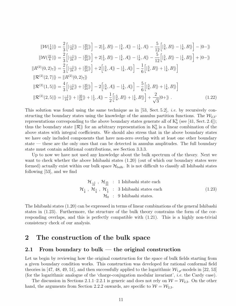
This solution was found using the same technique as in [53, Sect. 5.2], i.e. by recursively con-structing the boundary states using the knowledge of the annulus partition functions. The W2,3-representations corresponding to the above boundary states generate all of Kb
0 (see [41, Sect. 2.4]);thus the boundary state ‖R〉〉 for an arbitrary representation in Kb
0 is a linear combination of theabove states with integral coefficients. We should also stress that in the above boundary stateswe have only included components that have non-zero overlap with at least one other boundarystate — these are the only ones that can be detected in annulus amplitudes. The full boundarystate must contain additional contributions, see Section 3.3.3.
Up to now we have not used any knowledge about the bulk spectrum of the theory. Next wewant to check whether the above Ishibashi states (1.20) (out of which our boundary states wereformed) actually exist within our bulk space Hbulk. It is not difficult to classify all Ishibashi statesfollowing [53], and we find
H−124, H 35
24: 1 Ishibashi state each
H 18, H 5
8, H 1
3: 3 Ishibashi states each (1.23)
H0 : 9 Ishibashi states.
The Ishibashi states (1.20) can be expressed in terms of linear combinations of the general Ishibashistates in (1.23). Furthermore, the structure of the bulk theory constrains the form of the cor-responding overlaps, and this is perfectly compatible with (1.21). This is a highly non-trivialconsistency check of our analysis.
2 The construction of the bulk space
2.1 From boundary to bulk — the original construction
Let us begin by reviewing how the original construction for the space of bulk fields starting froma given boundary condition works. This construction was developed for rational conformal fieldtheories in [47, 48, 49, 51], and then successfully applied to the logarithmicW1,p-models in [22, 53](for the logarithmic analogue of the ‘charge-conjugation modular invariant’, i.e. the Cardy case).
The discussion in Sections 2.1.1–2.2.1 is generic and does not rely on W =W2,3. On the otherhand, the arguments from Section 2.2.2 onwards, are specific to W =W2,3.
11

2.1.1 The algebra of boundary fields
We want to explain more precisely what we mean by a consistent boundary theory. First we recallthat for eachW-representation U there exists a conjugate representation U∗ that is defined on thegraded dual of U [54, Def. 2.35]. The operation of taking the conjugate of a representation definesa contravariant functor from Rep(W) to itself which we denote by (−)∗.
With this definition we can then explain what we mean by aW-symmetric algebra of boundaryfields (or boundary algebra for short): it is a collection of data (Hbnd,m, η, ε) where (see also [53,Sect. 1.2])
1. Hbnd is the space of boundary fields and forms a W-representation.
2. m ∈ Hom(Hbnd ⊗f Hbnd,Hbnd) is an intertwiner describing the associative boundary OPE4.That is, if we denote the corresponding intertwining operator by Vm : Hbnd⊗CHbnd → Hbnd,for each ψ ∈ Hbnd we obtain a linear map Vm(ψ, x) from Hbnd to (a completion of) Hbnd,and the OPE ψ(x)ψ′(0) of two boundary fields ψ, ψ′ ∈ Hbnd is written as Vm(ψ, x)ψ′.
3. η : W → Hbnd is an injective W-intertwiner such that η(Ω) is the identity field in Hbnd.Since η is injective, the entire VOAW is contained in Hbnd, as is required for aW-symmetricboundary condition.
4. ε : Hbnd →W∗ is a W-intertwiner describing one-point functions of boundary fields. It hasto give rise to a non-degenerate and symmetric two-point function on the boundary.
We will sometimes just write Hbnd in place of (Hbnd,m, η, ε). Given a boundary algebra, then-point function of boundary fields ψ1, . . . , ψn ∈ Hbnd on the upper half plane is given by⟨
ψ1(x1) · · ·ψn(xn)⟩uhp
=⟨ε(Vm(ψ1, x1) · · ·Vm(ψn−1, xn−1)ψn
), Ω⟩, (2.1)
where we take xn = 0 and x1 > x2 > · · · > xn.
2.1.2 Bulk-boundary maps
For the rational theories and the W1,p-models one could define the bulk space as a solution to auniversal property. In order to formulate this construction, we need the notion of a bulk-boundarymap.
Fix a boundary algebra Hbnd and let H be a W ⊗C W-representation. By a bulk-boundarymap we mean a linear map β(−, y) : H → Hbnd (here y > 0, and we again suppress the algebraiccompletion of the target from the notation) which satisfies the following two conditions:
(i) β is compatible with the W-symmetry: Given φ ∈ H, the element β(φ, y) is to be thoughtof as an insertion of the bulk field φ on the upper half plane at position iy, expanded interms of boundary fields at position 0. The compatibility condition is formulated as follows.
4 Here ⊗f denotes the fusion product. By construction of ⊗f , for three W-representations R,S, U , the vectorspace of intertwining operators V (−, x) : R⊗C S → U (we suppress the formal variable and algebraic completion inthe notation of the target vector space) is canonically isomorphic to the space of W-intertwiners Hom(R⊗f S,U),see [54, Def. 3.18 & Prop 4.15].
12

Write H as a quotient H = H/Q, where H =⊕
aMa⊗C Na for some index set a and Q is a
sub-representation of H. Denote by βa the composition
βa(−, y) = Ma ⊗C Na → H H β(−,y)−−−→ Hbnd . (2.2)
Then we require thatβa(φ⊗C φ
′, y) = Vl(φ, iy)Vr(φ′,−iy)Ω , (2.3)
for appropriate intertwining operators Vr(−, x) : Na ×W → Na and Vl(−, x) : Ma × Na →Hbnd. Here, Vr(−, x)Ω can be taken to be just translation by x. In particular, the space of allmaps βa is isomorphic to Hom(Ma ⊗f Na,Hbnd). We denote by βa ∈ Hom(Ma ⊗f Na,Hbnd)the image of βa under that isomorphism.
(ii) β is central: Since β(φ, y) corresponds to a bulk field φ inserted at iy, an n-point correlatorof boundary fields involving β(φ, y) should be continuous when a boundary field is takenpast zero. This gives rise to the centrality condition: write H = H/Q as in (i). The mapβ(−, y) is called central iff for all ψ ∈ Hbnd
limx0
Vm(ψ, x)β(φ, y) = limx0
Vm(β(φ, y), x)ψ . (2.4)
This can also be expressed in terms of the braiding cU,V : U ⊗f V → V ⊗f U in the categoryof W-representations, using the component maps βa introduced in (i),
m (idHbnd⊗f βa) (cMa,Hbnd
⊗f idNa) = m (βa ⊗f idHbnd) (idMa ⊗f cHbnd,Na) . (2.5)
A graphical representation of condition (2.5) is5
Ma Hbnd Na
Hbnd
βa
m
Ma Hbnd Na
Hbnd
βa
m
= (2.6)
We will sometimes also refer to βa as a ‘bulk-boundary map’. In the non-logarithmic rationalcase, bulk-boundary maps where first systematically studied in [59, 60]; the centrality conditionamounts to [60, Fig. 9d]. In the framework of vertex operator algebras and intertwining operators,the bulk-boundary map and its categorical expression (2.5) have appeared in [61, Sect. 1.8 & 3.2].
5Here we use the usual graphical notation of braided tensor categories [58]; our diagrams are read from bottomto top.
13

2.1.3 Characterising the bulk space
After these definitions we can now explain how the bulk space of states could be characterised forthe rational theories [47, 48, 49, 51], and for theW1,p-models in the case of the ‘charge-conjugationmodular invariant’ [22, 53], the logarithmic analogue of the Cardy case
Let us fix a boundary algebra Hbnd. We consider pairs (H, β), where H is a W ⊗C W-representation and β : H → Hbnd is a bulk-boundary map. By an arrow f : (H, β) → (H′, β′)between two such pairs we mean a W ⊗C W-intertwiner f : H → H′ such that the diagram
H H′
Hbnd
//f
99999999
ββ′ (2.7)
commutes. The space of bulk fields Hbulk and the bulk-boundary OPE βbb(−, y) for the boundaryalgebra Hbnd are then defined to be a terminal object in the category formed by these pairs andarrows. In other words, the pair (Hbulk, βbb) has the property that for all other pairs (H′, β′) thereexists a unique W ⊗C W-intertwiner f : H′ → Hbulk such that we have β′ = βbb f : H′ → Hbnd.
A terminal object need not exist, but if it does, it is unique up to unique isomorphism. Indeed,for another terminal object (H′bulk, β
′bb), there are unique intertwiners Hbulk → H′bulk and H′bulk →
Hbulk which – again by uniqueness – have to compose to the identity.The bulk-boundary OPE βbb(−, y) is necessarily injective. To see this, note that if f : M →
Hbulk is anyW⊗CW-intertwiner such that βbbf = 0, then f is an arrow from (M, 0) to (Hbulk, β).As 0 is also an arrow between these pairs, by uniqueness we have f = 0. This shows that thepresent formulation is equivalent to the one given in [53, Sect. 3.1].
For the actual computations the simplest case (and in many situations the only tractable case)is to take as the boundary condition the ‘identity’ boundary condition, i.e. the boundary conditionwhose space of states just consists of the W-algebra itself. Such a boundary condition exists forthe W1,p-models [22, 53]. In that case, the objects of the category are (H, β), where β is a bulk-boundary map H → W . Since the image lies in W , the centrality condition (ii) in the definitionof the bulk-boundary map is trivial, and the problem simplifies considerably. This approach wassuccessfully applied to the W1,p-models in [53].
2.2 The proposal for the bulk space of the W2,3-model
Next we want to repeat a similar analysis for the case of the W2,3-model. Unfortunately, as wasalready mentioned earlier, the W2,3-model does not have an ‘identity brane’ whose space of statesonly consists of W2,3 itself. Thus we cannot directly apply the same method that worked for theW1,p-models. One could obviously try to apply the general formalism to a different boundarycondition, but then the centrality condition (ii) plays an important role, and we have not beenable to characterise the most general bulk-boundary maps in any useful way.
Instead we shall proceed slightly differently. By assumption, any W-symmetric boundarycondition hasW as a subalgebra in its space of boundary fields Hbnd. Since Hbnd is self-conjugate,it follows that W∗ can be obtained as a quotient of Hbnd. It seems reasonable to assume thatthere is at least one boundary condition, for which the disc correlator of a bulk and a boundary
14

field is already non-degenerate in the bulk entry if we take the boundary insertions only fromW . (This is the natural analogue of the ‘identity brane case’.) The two-point functions on theboundary define a natural pairing between W and W∗. The above supposition therefore impliesthat the bulk-boundary map is still injective after projecting from Hbnd toW∗. Obviously, for theW1,p-models W∗ ∼=W , and the distinction between W and W∗ is immaterial.
We thus propose that the natural analogue of the ‘identity brane’ situation is to consider bulk-boundary maps β : H → W∗ whose image is W∗, rather than W , and that the terminal objectwithin this category is our desired bulk space (Hbulk, βbb). As we shall explain in Section 2.3, itsatisfies a number of fairly non-trivial consistency conditions.
2.2.1 Characterising the terminal object
As advertised above, let us consider the category of pairs (H, β), where H is a W ⊗C W-representation, and β : H →W∗ is compatible with theW-symmetry, that is, it satisfies condition(i) of a bulk-boundary map as stated in Section 2.1.2. The arrows are intertwiners f : H → H′which make the diagram
H H′
W∗
//f
99999999
ββ′ (2.8)
commute. We want to find a terminal object (Hbulk, βbb) in this category. As in Section 2.1.2, theterminal object need not exist, but if it does it is unique and βbb is injective.
It was argued in [41, Sect. 5.1] that there is an isomorphism Hom(U, V ∗)→ Hom(U ⊗f V,W∗).The image of the natural isomorphism U → U∗∗ under this map provides a non-degenerate pairing
evU : U ⊗f U∗ −→W∗ (2.9)
for all representations U . Let VevU (−, x) : U × U∗ → W∗ be the corresponding intertwiningoperator. Non-degeneracy means that for all u ∈ U there is a u′ ∈ U∗ such that VevU (u, x)u′ 6= 0,and vice versa.
Suppose that W has a finite number of irreducible representations and that each of these hasa projective cover P(a). Let us denote by H the space H =
⊕aP(a)⊗C P(a)∗, where the direct
sum is over all irreducible representations, and define the map β =⊕
a VevP(a): H → W∗. Let
Hbulk = H/ ker(β) and let βbb : Hbulk →W∗ be the map induced by β on the quotient. We claim
(Hbulk, βbb) is a terminal object in the above category.
The proof proceeds analogously to the one in [53, Sect. 3.5]. Every representation H′ can bewritten as
H′ = H′/Q′ ; H′ =⊕a,b
NabP(a)⊗C P(b) , (2.10)
where Nab are multiplicities and Q′ is a sub-representation of the direct sum. Suppose that (H′, β′)is a pair in our category, where we write H′ as in (2.10). Denote the corresponding projection byπ′ : H′ → H′. If we define β′ = β′ π′, then π′ describes an arrow from (H′, β′) to (H′, β′).
15

Our first aim is to construct an arrow (H′, β′) → (Hbulk, βbb). To this end we denote therestriction of β′ to the k’th summand P(a) ⊗C P(b) → H′ by β′k. By definition of evP(a), thereexist intertwiners fa,b,k : P(b)→ P(a)∗ such that
β′k = VevP(a) (idP(a) ⊗C fa,b,k) . (2.11)
Then f =⊕
a
∑b,k idP(a) ⊗C fa,b,k : H′ → H provides an arrow f : (H′, β′)→ (H, β). We compose
this arrow with the projection (H, β) → (Hbulk, βbb) to give the desired arrow f ′ : (H′, β′) →(Hbulk, βbb).
Next we want to show that this gives rise to an arrow on (H′, β′). First we note that Q′ isequal to ker(π′), and thus also β′ vanishes on Q′. But β′ = βbb f ′ (as f ′ : H′ → Hbulk is an arrowin our category), and since βbb is injective, f ′ vanishes on Q′. Thus there is a well-defined mapg : H′ → Hbulk on the quotient, which provides the sought-after arrow (H′, β′) → (Hbulk, βbb).Since βbb is injective, this arrow is unique.
It remains to find a practical way to compute the kernel N = ker β of β : H → W∗ to obtainHbulk as a quotient. This can be done by the construction in [53, Sect. 3.3], which we brieflyreview. There we described N as the image of all possible maps of projectives P(i) ⊗C P(j), forall i, j, into N . For fixed i, j such a map takes the form h : P(i)⊗C P(j)→ H, h =
⊕a fa ⊗C g
∗a,
where fa : P(i)→ P(a) and ga : P(a)→ P(j)∗. Since
β h =⊕a
VevP(a) (fa ⊗C g
∗a) =
∑a
VevP(i)(idP(i) ⊗C (ga fa)∗
), (2.12)
βh is zero if and only if∑
a ga fa = 0. Since N itself is a quotient of a direct sum of P(i)⊗CP(j)with some multiplicities, the above construction produces the entire kernel.
If P(j)∗ ∼= P(j), a generic example of such maps fa and ga is found as follows. Let e : P(i)→P(j) be any morphism. Then(
P(i)e−→ P(j)
id−→ P(j) ∼= P(j)∗)
+(P(i)
id−→ P(i)−e−→ P(j) ∼= P(j)∗
)= 0 . (2.13)
Thus, the image of P(i)⊗C P(j)∗ under e⊗C id− id⊗C e∗ lies in N .
2.2.2 Projective covers
We now restrict our attention again to the caseW =W2,3. As we have just seen, the constructionof Hbulk relies on the existence of projective covers for all irreducible representations. For W(h)with h taking all values in (1.4) except h = 0, these were given in [41] to be (1.6). The argumentin [41] was based on the assumption that the projective cover of the irreducible representationW(−1
24) is W(−1
24) itself. Hence for every representation U that has a dual, also W(−1
24) ⊗f U is
projective (see Appendix B.1 for details). By the fusion rules in [41, App. A.4], this implies that theindecomposable representations listed in (1.6) are necessarily projective. From their compositionseries as given in Appendix A.1 one sees that they provide the projective covers of allW(h) exceptfor h = 0.
Regarding P(0), one first notes that the only representations R in (1.4) and (1.5) which allowfor a surjection R→W(0) are W(0), W and Q. It is verified in [41, App. A.3] that these are not
16

projective. On the other hand, in [55, Thm. 3.24] it is stated that under certain conditions on W ,including C1-cofiniteness, every irreducible W-representation has a projective cover. We do notknow ifW2,3 satisfies these conditions, but it seems plausible to us that it does (see also [44]). Wewill hence assume thatW(0) does have a projective cover. Using these assumptions as well as theresult of the recent calculation of Zhu’s algebra [46] it follows that P(0) has the composition series
W(0)→W(1)⊕W(2)→W(0)⊕ 2W(5)⊕ 2W(7)→W(1)⊕W(2)→W(0) . (2.14)
The derivation is given in Appendix B, and the corresponding embedding diagram can be foundin Appendix A.1.
2.2.3 Computing the Kernel
Next we want to work out (Hbulk, βbb) as defined in the previous subsection explicitly. Recall fromsection 2.2.1 that H is defined as H =
⊕aP(a) ⊗C P(a)∗. We want to determine the quotient
space Hbulk = H/ker(β), where
β =⊕a
VevP(a): H → W∗ . (2.15)
First we will show that one may choose representatives of vectors in Hbulk in
H(0)bulk =
⊕a
W(a)⊗C P(a)∗ , (2.16)
where W(a) is the top factor in the composition series of P(a). (This is very similar to whathappened in [28] and [53].) Consider some element W(i) ⊗C W(j) ⊂ P(a) ⊗C P(a)∗ in thecomposition series of H. Since P(i) is the projective cover of W(i), it follows that there existsan intertwiner e : P(i)→ P(a) such that the top factor W(i) in the composition series of P(i) ismapped to the given W(i) ⊂ P(a). By (2.13) it then follows that the image of
e⊗C idP(a) − idP(i) ⊗C e∗ (2.17)
lies in the kernel of β. Thus in Hbulk, any vector inW(i)⊗C W(j) ⊂ P(a)⊗C P(a)∗, whereW(i) isnot the top component of P(a), lies in the same equivalence class as a vector inW(i)⊗C e
∗(W(j)) ⊂P(i) ⊗C P(i)∗, where W(i) is the top component of P(i). Thus we have shown that Hbulk is at
most as big as H(0)bulk.
We can collect the terms of H into sectors
H = H0 ⊕ H 18⊕ H 5
8⊕ H 1
3⊕ H 35
24⊕ H−1
24, (2.18)
with
H−124
=W(−124
)⊗C W(−124
)∗ H 3524
=W(3524
)⊗C W(3524
)∗
H 13
=⊕
a= 13, 10
3
P(a)⊗C P(a)∗ H 58
=⊕
a= 58, 21
8
P(a)⊗C P(a)∗ (2.19)
H 18
=⊕
a= 18, 33
8
P(a)⊗C P(a)∗ H0 =⊕
a=0,1,2,5,7
P(a)⊗C P(a)∗ .
17

It is easy to see that the kernel of β does not mix the different sectors in (2.18), and we maytherefore consider each of them in turn. It follows from the arguments of [53, Sect. 4.3 & App. D]that in all sectors, except possibly for H0, all relations of the quotient space Hbulk = H/ker(β) aretaken into account by (2.17) and that Hbulk is isomorphic (as an (Ldiag
0 , Ldiag0 )-graded vector space,
see (1.1)) to H(0)bulk. We believe that this will also be the case for H0, but we have no proof. We
therefore conjecture that H(0)bulk is not just an upper bound for Hbulk, but actually isomorphic to it.
This gives then the explicit description of Hbulk that was advertised before. (The bulk-boundarymap βbb is the one induced from β under the quotient map H Hbulk.)
2.3 Properties of the resulting bulk space
Next we want to describe the resulting bulk space Hbulk in some more detail. First we want toexplain how W ⊗C W acts on it. Given that we have a description of Hbulk as a quotient by Nof H, this can now be easily deduced. Since H has a decomposition as in (2.18), we get a similardecomposition for Hbulk, which we write as
Hbulk = H/N = H0 ⊕H 18⊕H 5
8⊕H 1
3⊕H−1
24⊕H 35
24. (2.20)
In order to describe the resulting structure we analyse, sector by sector, their composition series,following the method outlined in Section 1.3. This is to say, we identify first the largest directsum of irreducible subrepresentations; then we quotient by these and find the largest direct sum ofirreducible subrepresentations in the quotient, etc. The situation is obviously simplest for H−1/24
and H35/24 since they are already, by themselves, irreducible. As a consequence, the quotient istrivial for these sectors, and the resulting composition series just consists of one term.
2.3.1 The edge of the Kac table
The situation is more interesting for those sectors that come from the ‘edge of the Kac table’,i.e. the sectors H1/8, H1/3 and H5/8. In the following we shall only show the calculation for thefirst case (h = 1
8) — the other cases then follow upon replacing 1
8, 33
8 with 5
8, 21
8 or 1
3, 10
3,
respectively.As we have explained above, the representatives are described by H(0)
1/8, see eq. (2.16). It is
then not difficult to show that the maximal fully reducible subrepresentation of M1(18) = H1/8 is
given by
R1(18) =
⊕i= 1
8, 33
8
W(i)⊗C W(i) , (2.21)
where W(i) comes from the bottom entry in P(i).Next, we consider the quotient M2(1
8) = M1(1
8)/R1(1
8), and repeat the analysis. The maximal
fully reducible subrepresentation of M2(18) is
R2(18) = 2W(1
8)⊗C W(33
8) ⊕ 2W(33
8)⊗C W(1
8) . (2.22)
18

These arise from the middle lines in the embedding diagrams of the corresponding projective coversP(i). Finally, the maximal fully reducible subrepresentation of M3(1
8) = M2(1
8)/R2(1
8) equals
R3(18) =
⊕i= 1
8, 33
8
W(i)⊗C W(i) , (2.23)
which comes from the top entries of P(i). Thus we obtain precisely the composition series givenin (1.18).
2.3.2 The interior of the Kac table
This leaves us with the sector H0, for which the analysis is more complicated. Proceeding asbefore we find that the maximal fully reducible subrepresentation of M1(0) = H0 is given by
R1(0) =⊕
i=0,1,2,5,7
W(i)⊗C W(i) . (2.24)
As before, these states arise from the bottom component in P(i)∗.Next, we find that the maximal fully reducible subrepresentation of M2(0) = M1(0)/R1(0) is
R2(0) =(W(1)⊕W(2)
)⊗C(2 W(5)⊕ 2 W(7)⊕ W(0)
)⊕(W(5)⊕W(7)
)⊗C(2 W(2)⊕ 2 W(1)
)(2.25)
⊕W(0)⊗C(W(1)⊕ W(2)
),
while that of M3(0) = M2(0)/R2(0) is
R3(0) =W(1)⊗C(2 W(1)⊕ 4 W(2)
)⊕W(2)⊗C
(2 W(2)⊕ 4W(1)
)⊕W(0)⊗C
(W(0)⊕ 2 W(5)⊕ 2 W(7)
)(2.26)
⊕W(5)⊗C(2 W(0)⊕ 2 W(5)⊕ 4 W(7)
)⊕W(7)⊗C
(2 W(0)⊕ 2 W(7)⊕ 4 W(5)
).
Similarly, the maximal fully reducible subrepresentation of M4(0) = M3(0)/R3(0) is R4(0) =R2(0), while that of M5(0) = M4(0)/R4(0) equals R5(0) = R1(0). This agrees precisely with whatwe claimed in (1.19).
2.3.3 Consistency conditions
Finally, let us comment on the consistency conditions our answer satisfies. None of the propertiesdiscussed below is built into our ansatz from the start, and they give strong support to ourproposed bulk space.
Modular invariance: Given the composition series (1.16), (1.18) and (1.19), it is straightforwardto work out the partition function of Hbulk, resulting in
Z(q) =∑
i χW(i)(q) · χP(i)(q)
= (qq)−1/24 + 3 + 2(qq)1/8 + 2(qq)1/3 + (q+q) · (qq)−1/24 + 2(q+q) + · · · ,(2.27)
19

where the sum runs over all 13 irreducibles (including W(0)). This partition function was alreadyproposed in [41, Sect. 4], at least up to the multiplicity of (qq)0, which was left as an arbitrarypositive integer there. As was mentioned in [41], Z(q) is modular invariant (see also [35]).
Self-conjugacy: The space of bulk states Hbulk is actually isomorphic to its conjugate represen-tation, H∗bulk. This is necessary in order for the bulk theory to have a non-degenerate (bulk)two-point function.
Stress tensor: Curiously, the composition series (1.19) of Hbulk shows that Hbulk does not containW ⊗C W as a sub-representation. To see this we note that the composition series of W ⊗C W is
0 2
0 1 0
2 0 0
−→0 2
0 0 1
2 1 0
−→0 2
0 0 0
2 0 1
. (2.28)
In order to embedW⊗C W into Hbulk, we need to map the level 0 subspace W(0)⊗C W(0) to thesummand W(0)⊗C W(0) of Hbulk at level 2. However, the composition series (A.1) of P(0) showsthat from there one can reach e.g.W(0)⊗CW(1), which is not contained inW⊗CW . Nonetheless,Hbulk does still contain a holomorphic field of weight (2, 0) and an anti-holomorphic field of weight(0, 2), which form the candidate stress tensor. For example, a representative of the equivalenceclass of the state of weight (2, 0) at level 3 of Hbulk (see (1.19)) isW(2)⊗C W(0) ⊂ P(2)⊗C P(2)∗,where W(0) sits at level 3. Acting with L−1 gives a state of weight (2, 1), where the factor withweight 1 has to be at level 4 of P(2), which, however, does not contain such a state. Thus thestate of weight (2, 0) really defines a holomorphic field.
As an aside, we note that this argument also suggests that the the state of weight (1, 0) at level3 of Hbulk is not holomorphic, as acting with L−1 on its representative W(1)⊗C W(0) ⊂ P(1)⊗CP(1)∗, where W(0) sits at level 3, gives a state of weight (1, 1) inW(1)⊗C W(1) ⊂ P(1)⊗C P(1)∗,where W(1) sits at level 4, and it seems highly plausible that this state is nonzero.
Boundary states: As a final consistency check, we can study the boundary states one can constructwithin Hbulk. In particular, as we shall show in the following section, we are able to reproduce theboundary theory of [41] in this manner.
3 The boundary state analysis
In this section we want to study how the boundary conditions that were proposed in [41] fit intothe present analysis. In particular, we want to show how the corresponding boundary states canbe constructed in our proposed bulk theory Hbulk.
3.1 Reconstructing the boundary states
Let us begin by identifying the Ishibashi states and their overlaps that reproduce the annuluspartition functions of [41]; this first part of the analysis does not require any detailed knowledgeabout the bulk space Hbulk. The basic idea of the analysis is simple. Given the proposal of [41],
20

we know the annulus partition functions in the ‘open string sector’. More specifically, if R and R′label two consistent boundary conditions, then the open string annulus amplitude is simply
χR⊗fR′∗(q) , (3.1)
where χS denotes the character of S and q = exp(−2πi/τ) is open string modular parameter.Thus the overlap of the corresponding boundary states ‖R〉〉 and ‖R′〉〉 must equal
〈〈R‖qL0+L0‖R′〉〉 = χR⊗fR′∗(q) , (3.2)
i.e. the modular S-transform of (3.1) — see appendix A.2 for explicit formulae, or [35, 38] for theformula for general Wp,q-models.
By considering the different powers of q that appear in (3.2), it is clear which contributionarises from which sector of Hbulk in (2.20). We can thus identify the overlaps of the variousdifferent Ishibashi states that appear. As was explained in Section 1.4, the annulus amplitudescan be described in terms of ten Ishibashi states, reflecting the fact that the overlaps have a 2-dimensional null ideal, see eq. (1.9). We should stress, however, that this does not mean that theactual boundary states can be written in terms of these ten Ishibashi states. It only means thatfor the calculation of the annulus amplitudes, only the coupling to these ten Ishibashi states isrequired. (In fact, it seems natural to assume that the actual boundary states will depend on twomore Ishibashi states, but we have not managed to prove this.)
So far, we have not used any detailed information about the structure of the bulk spectrum.The non-trivial consistency condition now arises from the requirement that the Ishibashi states(1.20) and their overlaps (1.21) can indeed be obtained within Hbulk. In order to see that this ispossible we begin by classifying the most general Ishibashi states in Hbulk.
3.2 The Ishibashi states
As was explained in [53, Section 5.1], we may think of the Ishibashi states in terms of ‘Ishibashimorphisms’. Indeed, each Ishibashi state defines (and is defined by) a ‘bulk-boundary pairing’Hbulk ×W → C that is compatible with the W action. Since the bulk space Hbulk is the quotientof H by N , the space of all Ishibashi intertwiners consists of those bulk-boundary pairings on Hthat vanish on N . It was furthermore shown in [53] that every such bulk boundary pairing canbe written as
bρ(u⊗C v, w
)=∑a
(evP(a)(ρa(ua), va)
)(w) , (3.3)
where ρ is an intertwiner ρ =⊕
a ρa : P(a)→ P(a). Here u⊗C v =⊕
a ua ⊗C va ∈ H, and w ∈ W .Furthermore, as also explained in [53], the condition to vanish onN can be analysed by very similarmethods as above in Section 2.2.1. The bulk boundary map bρ vanishes on N if and only if∑
a
ga ρa fa = 0 (3.4)
for all fa : P(i)→ P(a) and ga : P(a)→ P(j) such that (⊕
a fa ⊗C g∗a)(P(i)⊗C P(j)∗) lies in N .
As is familiar from the usual rational case, we can analyse the Ishibashi states sector by sector.Again, the situation is easiest for the sectors H−1/24 and H35/24, corresponding to the irreducible
21

representations at the corner of the Kac table. In either case Schur’s lemma implies that there isonly a one-dimensional space of intertwiners, and since N only intersects these sectors in 0, thereis no additional constraint to worry about. Thus we have one Ishibashi state from each of thesetwo sectors.
3.2.1 The edge of the Kac table
The situation is more interesting for the sectors from the ‘edge of the Kac table’, i.e. the sectorsH1/8, H5/8 and H1/3. For concreteness, let us again only consider the case of H1/8; the situationin the other sectors is completely analogous. First we recall that
H 18
=(P(1
8)⊗C P(1
8)∗)⊕(P(33
8)⊗C P(33
8)∗). (3.5)
As was explained in [41], the space of intertwiners ρ : P(18)→ P(1
8) is two-dimensional, and simi-
larly for P(338
). Thus, in addition to the identity intertwiner ida, there is one linearly independentintertwiner which we denote by na ≡ ea→a2 ; our notation for the intertwiners is explained in Ap-pendix A.1. The intertwiner ida acts as the identity on P(a), and as zero on the other summandin (3.5), and similarly for na. In total, we therefore have four such intertwiners, and we write themost general ansatz as
ρ = ρ 18⊕ ρ 33
8=⊕
a= 18, 33
8
A(1)a ida + A(2)
a na . (3.6)
The space N by which we have to quotient out H1/8 is generated by(ea→b1;α ⊗C id− id⊗C (ea→b1;α )∗
) (P(a)⊗C P(b)∗
), (3.7)
where either (a = 18
and b = 338
) or (a = 338
and b = 18), and α denotes the two different choices of
such intertwiners. (This is because the other relations of the form (2.13), involving intertwinersof higher degree, are a consequence of these.) By (3.4), the intertwiner ρ vanishes on (3.7) if andonly if for each α we have on P(a)
ρb ea→b1;α − (ea→b1;α ) ρa = 0 . (3.8)
Thus there is a three-dimensional solution space with basis
ρ(1) = id18 + id
338 , ρ(a,2) = na , a = 1
8, 33
8, (3.9)
since ea→b1;α na = nb ea→b1;α = 0. This analysis is completely analogous to the discussion in [53].
3.2.2 The interior of the Kac table
This leaves us with analysing the Ishibashi morphisms in the sector H0, corresponding to the‘interior of the Kac table’. The following calculations make frequent reference to the embeddingdiagrams (A.1)-(A.3) of the projective representations P(0),P(1),P(2),P(5) and P(7), and ofour conventions regarding intertwiners described there. As is apparent from these embedding dia-grams, the space of intertwiners of each of the projective representations P(a) with a ∈ 1, 2, 5, 7
22

is 4-dimensional. For each such P(a) let ida be the identity intertwiner, while ea→a4 denotes theunique intertwiner of degree four. The remaining two intertwiners have degree 2, and will bedenoted by ea→a2;α , where α takes the appropriate two values out of 1, 2, 5, 7, as explained inAppendix A.1. The most general ansatz for an intertwiner P(a)→ P(a), a = 1, 2, 5, 7 is therefore
ρa = Aida ida +
∑α
Aαa ea→a2;α + A4
a ea→a4 . (3.10)
For the case of P(0), the space of intertwiners from P(0) to itself is 3-dimensional; apart from theidentity intertwiner id0, there are the intertwiners e0→0
2 and e0→04 of degree 2 and 4, respectively.
The most general ansatz for an intertwiner P(0)→ P(0) is therefore
ρ0 = Aid0 id0 + A2
0 e0→02 + A4
0 e0→04 . (3.11)
Before taking into account the constraints coming from N , the number of intertwiners we need toconsider in the sector H0 is therefore 19 = 4× 4 + 3.
The intersection of N with H0 is again generated by the relations of the form (2.13) involvingintertwiners of degree 1 (
ea→b1;β ⊗C idb − ida ⊗C (ea→b1;β )∗) (P(a)⊗C P(b)∗
)(e0→d
1 ⊗C idd − id0 ⊗C (e0→d1 )∗
) (P(0)⊗C P(d)∗
)(3.12)(
ed→01 ⊗C id0 − idd ⊗C (ed→0
1 )∗) (P(d)⊗C P(0)∗
),
where (a, b) = (1, 5), (1, 7), (2, 5), (2, 7) or (a, b) = (5, 1), (7, 1), (5, 2), (7, 2) and d ∈ 1, 2. By(3.4), the intertwiner ρ vanishes on (3.7) if and only if
ρb ea→b1;β − ea→b1;β ρa = 0 on P(a) ,
ρd e0→d1 − e0→d
1 ρ0 = 0 on P(0) , (3.13)
ρ0 ed→01 − ed→0
1 ρd = 0 on P(d) .
Evaluating the first equation of (3.13) we get
0 = ρb ea→b1;β − ea→b1;β ρa
=(Aidb idb +
∑η
Aηb eb→b2;η + A4
b eb→b4
) ea→b1;β − ea→b1;β
(Aida ida +
∑η
Aηaea→a2;η + A4
a ea→a4
)= (Aid
b − Aida )ea→b1;β +
∑γ
(∑η
AηbCγηβ −
∑η
AηaCγβη
)ea→b3;γ , (3.14)
where we have used that eb→b4 ea→b1;β = 0 = ea→b1;β ea→a4 , as well as defined the structure constantsvia (see Appendix A.1 for some examples)
eb→b2;α ea→b1;β =∑γ
Cγα,β e
a→b3;γ , ea→b1;β ea→a2;α =
∑γ
Cγβ,α e
a→b3;γ . (3.15)
23

The second and third equations of (3.13) lead to equivalent relations. Concentrating on the formerwe obtain
0 = ρd e0→d1 − e0→d
1 ρ0
= (Aidd idd + A5
d ed→d2,5 + A7
d ed→d2,7 + A4
d ed→d4 ) e0→d
1 − e0→d1 (Aid
0 id0 + A20 e
0→02 + A4
0 e0→04 )
= (Aidd − Aid
0 )e0→d1 + (A5
d + A7d − A2
0)e0→d3 , (3.16)
where we have again used that ed→d4 e0→d1 = 0 = e0→d
1 e0→04 . A basis for the space of solutions
is given by the following nine Ishibashi morphisms6
ρ(id) = id0 + id1 + id2 + id5 + id7
ρ(µ) = e0→02 + e1→1
2,7 + e2→22,5 + e5→5
2,2 + e7→72,1
ρ(ν) = e0→02 + e1→1
2,5 + e2→22,7 + e5→5
2,1 + e7→72,2 (3.17)
ρ(δ) = e2→22,5 − e2→2
2,7 + e5→52,2 − e7→7
2,2
ρ(σi) = ei→i4 i = 0, 1, 2, 5, 7 .
3.3 Overlaps of Ishibashi states
In order to identify the Ishibashi states (1.20) with linear combinations of the Ishibashi statescorresponding to the intertwiners (3.17), we need to determine the different overlaps between thelatter. Obviously, the overlaps between Ishibashi states from different sectors vanish, but sincethere is generically more than one Ishibashi state in each sector, the relative overlaps between themare more complicated. The first step in identifying the structure of these overlaps is to understandthe relation between the Ishibashi morphisms ρ and the corresponding Ishibashi states |ρ〉〉, thoughtof as elements in a completion of Hbulk. Suppose that w ∈ Hbulk is an arbitrary bulk state, thenwe have
bρ(w,Ω) = B(|ρ〉〉, w) , (3.18)
where B(−,−) is the bulk 2-point function and bρ is defined by (3.3). That |ρ〉〉 is annihilated by(Wm − (−1)hW W−m) is related to the fact that bρ(−,Ω) is a chiral 2-point block on the sphere(see e.g. [53, App. A]). Since the bulk 2-point function is non-degenerate, it follows that ρ deter-mines uniquely the corresponding Ishibashi state |ρ〉〉, and vice versa. Given the knowledge of thecorresponding Ishibashi state we can then work out the cylinder overlaps since we have
〈〈ρ1|qL0+L0|ρ2〉〉 = B(|ρ1〉〉, qL0+L0|ρ2〉〉
). (3.19)
It follows from the definition of (3.3) that bρ(u⊗C v,Ω) is only nonzero provided that ρa(ua) and vacontain summands that are conjugate to one another. Here we have written u⊗C v =
∑a ua⊗C va
with ua ⊗C va ∈ P(a)⊗C P(a)∗.As regards the bulk 2-point function B(−,−), we choose the following convention. Fixing a
bulk 2-point function is equivalent to giving an isomorphism Hbulk → H∗bulk, which one can then
6We believe that by an appropriate rescaling of the intertwiners, the coefficients Cγα,β and Cγβ,α can be chosento be either zero or one. This was used to arrive at (3.17).
24

precompose with the canonical pairing Hbulk ×H∗bulk → C. There is no unique choice, but thereis a preferred such isomorphism: if we keep the vector space decomposition implicit in (1.19), theconjugation map flips the direction of all arrows, and effectively turns the composition diagramupside down. We pick the isomorphism which maps the level 0 states of Hbulk to states of H∗bulk
which have components only at level 0 (and not also at levels 2 and 4). With this choice, the bulk2-point function is non-vanishing only for combinations of states at opposite points in the bulkcomposition series.
Combining these two considerations we can then determine the components of the bulk com-position series in which the Ishibashi state has non-trivial components, as we shall now see.
3.3.1 The corner of the Kac table
Let us begin with the Ishibashi states from the sectors H−1/24 and H35/24. For these sectors theIshibashi morphisms are proportional to the identity and the Ishibashi states are just those builtupon the highest weight states. We can then normalise the two resulting Ishibashi states |−1
24〉〉
and |3524〉〉 such that their overlaps are
〈〈−124| qL0+L0 |−1
24〉〉 =√
3χW(−124
)(q) and 〈〈35
24| qL0+L0 |35
24〉〉 = −
√3χW(
3524
)(q) , (3.20)
in agreement with (1.21).
3.3.2 The edge of the Kac table
For the sectors along the ‘edge of the Kac table’, let us first work out the non-trivial componentsof the Ishibashi states. As in the previous sections we shall do this explicitly in the H1/8 sector;the analysis in the other edge sectors is similar. The Ishibashi morphism bρid is non-vanishing onu⊗C v ∈ H1/8 provided that the components ua⊗C va are conjugate to one another in P(a)⊗C P(a).If we choose the representatives ua⊗C va according to (2.16), then ua lies in the top W(a) at level0 in P(a). In order for va to be conjugate to ua it must then lie in the bottom W(a), i.e. at level2 in P(a)∗. In terms of the analysis of Section 2.3.1, it then follows that u ⊗C v must lie in thegrey components of the composition series,
bρ(id) 6= 0 only on
18
338
18
1 0338
0 1
−→
18
338
18
0 2338
2 0
−→
18
338
18
1 0338
0 1
, (3.21)
where we have used the same notation as in (1.18). The corresponding Ishibashi state (that weshall denote by |id〉〉) then has non-zero components in the conjugate sectors.
|id〉〉 ∈
18
338
18
1 0338
0 1
−→
18
338
18
0 2338
2 0
−→
18
338
18
1 0338
0 1
. (3.22)
25

The analysis for the Ishibashi morphism ρ(a,2) is similar. Again, ρ(a,2) is non-vanishing onu ⊗C v ∈ H1/8 provided that na(u) is conjugate to v. Since na(u) maps the top W(a) to thebottom W(a) in P(a), it follows that u⊗C v has to have non-zero components in the sectors
bρ(1/8,2) 6= 0 only on
18
338
18
1 0338
0 1
−→
18
338
18
0 2338
2 0
−→
18
338
18
1 0338
0 1
(3.23)
and
bρ(33/8,2) 6= 0 only on
18
338
18
1 0338
0 1
−→
18
338
18
0 2338
2 0
−→
18
338
18
1 0338
0 1
, (3.24)
respectively. The corresponding Ishibashi states will be denoted by |n1/8〉〉 and |n33/8〉〉, and theymust have non-trivial components in the conjugate sectors, i.e. in
|n1/8〉〉 ∈
18
338
18
1 0338
0 1
−→
18
338
18
0 2338
2 0
−→
18
338
18
1 0338
0 1
(3.25)
and
|n33/8〉〉 ∈
18
338
18
1 0338
0 1
−→
18
338
18
0 2338
2 0
−→
18
338
18
1 0338
0 1
. (3.26)
Given this information, we can then directly work out the non-trivial overlaps between theseIshibashi states. For example, for the overlaps of |n1/8〉〉 (or |n33/8〉〉) with themselves vanish, sinceboth of these states only have a component in the ‘bottom’ factor, but none in the conjugate ‘top’factor. On the other hand, the overlap with |id〉〉 is non-zero, and we can choose the normalisationof |n1/8〉〉 and |n33/8〉〉 such that
〈〈id|qL0+L0|n1/8〉〉 = χW(
18
)(q) 〈〈id|qL0+L0 |n33/8〉〉 = χ
W(338
)(q) . (3.27)
Let us decompose the action of L0 on a representation R as L0 = Ldiag0 + Lnil
0 , where Lnil0
denotes the nilpotent part. Since for a mode Wm of a homogeneous generator W of W2,3 we have
[L0,Wm] = −mWm as well as [Ldiag0 ,Wm] = −mWm (after all, Ldiag
0 just gives the grading of Rand Wm is a map of degree −m), it follows that [Lnil
0 ,Wm] = 0, i.e. the nilpotent part of L0 is anintertwiner from R to itself. In particular, if |i〉〉 is an Ishibashi state, so is (Lnil
0 + Lnil0 )n|i〉〉 for any
n ≥ 0.The above discussion, together with the observations in (3.22), (3.25) and (3.26) shows that
(Lnil0 + Lnil
0 )|id〉〉 is again an Ishibashi state, and it has to be a linear combination of |n1/8〉〉 and|n33/8〉〉. We can choose the normalisation of |id〉〉 such that
1
2π(Lnil
0 + Lnil0 )|id〉〉 = |n1/8〉〉+ α33/8|n33/8〉〉 , (3.28)
26

for some constant α33/8 ∈ C. We should note that α33/8 is in principle determined by the structureof Hbulk, but that with our current limited understanding of the latter we cannot actually calculateit from first principles. In any case it follows that
〈〈id|qL0+L0|id〉〉 = iτ(χW(
18
)(q) + α33/8 · χW(
338
)(q)). (3.29)
If we now set
|18, A〉〉 =
i√3|id〉〉 , |1
8, B〉〉 = −2i
(|n1/8〉〉+ |n33/8〉〉
), α33/8 = −2 , (3.30)
we precisely reproduce the overlaps (1.21).We should also mention that the two Ishibashi states in (3.30) are characterised by the property
that their overlaps do not lead to any τ = −1/τ terms in the open string. Indeed, the additionallinear combination, which we could take to be |1
8, C〉〉 = |n1/8〉〉−|n33/8〉〉 cannot enter the boundary
state construction since it leads, in the open string loop diagram, to a term proportional to τ . Forexample, we find
〈〈18, A|qL0+L0|1
8, C〉〉 =
i√3
(χW(
18
)(q)− χ
W(338
)(q))
(3.31)
= − i
18
(χW(
18
)(q) + χ
W(338
)(q))
+τ
3√
3
(χW(
18
)(q)− 2χ
W(338
)(q))
+ (contributions from other sectors) ,
where τ = −1/τ is the modular parameter in the open string channel. The situation is thereforecompletely analogous to what was found in [53] for the W1,p-models.
The analysis in the other two sectors is essentially identical. Indeed, the analogues of (3.27)and (3.29) hold also for the Ishibashi states in H5/8 and H1/3, respectively, and this determinestheir overlaps up to the constants α21/8 and α10/3 as in (3.28). The Ishibashi states of (1.20) canthen be identified with
|58, A〉〉 = i
√23|id〉〉 |5
8, B〉〉 = −i
√2(|n5/8〉〉+ |n21/8〉〉
)(3.32)
|13, A〉〉 = 3
14
√2 |id〉〉 |1
3, B〉〉 = 3−
34
√2(|n1/3〉〉+ |n10/3〉〉
),
and we reproduce precisely the overlaps (1.21) provided that
α21/8 = −12, α10/3 = −1 . (3.33)
The third Ishibashi state in each of these sectors cannot contribute to the boundary states sinceit would lead to terms proportional to τ in the open string channel.
3.3.3 The interior of the Kac table
It therefore only remains to identify the Ishibashi states with components in H0, the ‘interior ofthe Kac table’. The Ishibashi morphism bρ(id) is non-vanishing for u⊗C v ∈ H0 provided that the
27

left and right tensor factor of the representatives in H0 are conjugate to one another. By the samelogic as above, this can only be the case provided that u⊗C v lies in the grey components
0 1 2 5 7
0 1
1 1
2 1
5 1
7 1
bρ(id) 6= 0 only on , (3.34)
where the empty squares are the remaining composition factors of (1.19), which we have left blankto keep the notation compact. The corresponding Ishibashi state |id〉〉 therefore has non-vanishingcomponents in the conjugate sectors
0 1 2 5 7
0 1
1 1
2 1
5 1
7 1
|id〉〉 ∈ . (3.35)
The Ishibashi morphisms bρ(σi) are non-vanishing for u⊗C v ∈ H0 provided that ρ(σi)(u) is conjugate
to v, i.e. provided that u⊗C v lies in theW(i)⊗CW(i) component at level 0 of the H0 compositionseries, e.g. for i = 2
0 1 2 5 7
0 1
1 1
2 1
5 1
7 1
bρ(σ2) 6= 0 only on . (3.36)
The corresponding Ishibashi state |σ2〉〉 must therefore have a non-vanishing component in theconjugate sector
0 1 2 5 7
0 1
1 1
2 1
5 1
7 1
|σ2〉〉 ∈ . (3.37)
The analysis for the other Ishibashi states |σi〉〉 for i = 0, 1, 5, 7 is similar, with W(2) ⊗C W(2)being replaced by W(i)⊗C W(i).
Finally, we consider the Ishibashi morphisms bρ(µ) , bρ(ν) and bρ(δ) . For them the analysis is morecomplicated because of the multiplicities of 2 on the diagonal of the third factor of the compositionseries (1.19). In (2.16) these two components come from W(a)⊗C W(a), where W(a) lies at level0, while W(a) lies on the very left or very right at level 2 in P(a)∗; we shall therefore denote these
28

sectors by ` and r, respectively. Note that the sector labelled by ` is conjugate to that labelled byr, and vice versa. With this notation, we have
0 1 2 5 7
0 1
1 `
2 `
5 `
7 `
bρ(µ) 6= 0 only on , (3.38)
0 1 2 5 7
0 1
1 r
2 r
5 r
7 r
bρ(ν) 6= 0 only on , (3.39)
0 1 2 5 7
0 1
1 2
2 2
5 `
7 r
bρ(δ) 6= 0 only on . (3.40)
The above diagrams imply in turn that the corresponding Ishibashi states must have non-vanishingcomponents in
|µ〉〉 ∈
0 1 2 5 7
0 1
1 r
2 r
5 r
7 r
, (3.41)
|ν〉〉 ∈
0 1 2 5 7
0 1
1 `
2 `
5 `
7 `
, (3.42)
|δ〉〉 ∈
0 1 2 5 7
0 1
1 2
2 2
5 r
7 `
. (3.43)
29

This predicts the following overlaps up to a number of constants that cannot be determined directlyin this manner
〈〈id|qL0+L0|id〉〉 = τ 2(α0 χW(0)(q) + α1 χW(1)(q) + α2 χW(2)(q) + α5 χW(5)(q) + α7 χW(7)(q)
)〈〈id|qL0+L0|µ〉〉 = τ
(βµ0 χW(0)(q) + βµ1 χW(1)(q) + βµ2 χW(2)(q) + βµ5 χW(5)(q) + βµ7 χW(7)(q)
)〈〈id|qL0+L0|ν〉〉 = τ
(βν0 χW(0)(q) + βν1 χW(1)(q) + βν2 χW(2)(q) + βν5 χW(5)(q) + βν7 χW(7)(q)
)〈〈id|qL0+L0|δ〉〉 = τ
(βδ2 χW(2)(q) + βδ5 χW(5)(q) + βδ7 χW(7)(q)
)〈〈id|qL0+L0|σi〉〉 = χW(i)(q)
〈〈µ|qL0+L0|µ〉〉 = αµ χW(0)(q) , 〈〈ν|qL0+L0|ν〉〉 = αν χW(0)(q)
〈〈δ|qL0+L0|δ〉〉 = αδ χW(2)(q)
〈〈µ|qL0+L0|ν〉〉 = γµν0 χW(0)(q) + γµν1 χW(1)(q) + γµν2 χW(2)(q) + γµν5 χW(5)(q) + γµν7 χW(7)(q)
〈〈µ|qL0+L0|δ〉〉 = γµδ2 χW(2)(q) + γµδ7 χW(7)(q)
〈〈ν|qL0+L0|δ〉〉 = γνδ2 χW(2)(q) + γνδ5 χW(5)(q) .
Some of these constants can be fixed by rescaling the Ishibashi states appropriately. Note that〈〈δ|qL0+L0|δ〉〉 probably vanishes (i.e. αδ = 0) because the two contributions from the 2’s in themiddle sector appear to cancel against each other, see (3.17).
Comparing to (1.21), we see that the Ishibashi states that enter the boundary state analysiscan be identified with
|0+〉〉 = |µ〉〉 and |0−〉〉 = |ν〉〉 (3.44)
provided that αµ = αν = 12, γµν0 = 1
2, and γµνj = 1 for j = 1, 2, 5, 7. Thus we can again obtain all
the relevant Ishibashi states within Hbulk.As before we can also ask whether there are additional Ishibashi states that could contribute to
consistent boundary states. By a straightforward calculation, using the modular transformationproperties of Appendix A.2, one can check that neither |id〉〉 nor |δ〉〉 can appear in boundary statessince 〈〈id|qL0+L0|id〉〉 and 〈〈µ|qL0+L0|δ〉〉 both lead to τ terms in the open string loop diagrams. Onthe other hand, a similar argument does not apply to the Ishibashi states |σi〉〉 since their relativeoverlaps, as well as their overlaps with |µ〉〉 and |ν〉〉 all vanish. Thus these Ishibashi states donot contribute to the cylinder diagrams, and we cannot decide whether they appear in boundarystates based on cylinder diagrams alone.
Given that the subgroup Kb0 of the Grothendieck group is 12-dimensional but only ten Ishibashi
states are required for the description of the cylinder diagrams, we suspect that at least certainlinear combinations of the |σi〉〉 also contribute to the boundary states. In fact, this is evenrequired in order for the bulk-boundary map to be non-degenerate in the bulk entry. To see thiswe observe that the bulk states from the top level in H0 only contribute in overlaps with the |σi〉〉Ishibashi states, see in particular eq. (3.36). Thus if the |σi〉〉 Ishibashi did not appear in any ofthe boundary states, all bulk-boundary maps would vanish on these top states, in contradictionwith the assumed non-degeneracy. However, since the |σi〉〉 Ishibashi states do not contribute toany cylinder diagrams the above analysis does not determine their coefficients.
30

4 Conclusion
In this paper we have made a proposal for the bulk space for the ‘charge conjugation’ modularinvariant of the logarithmic W2,3 triplet model. The basic idea of our construction is to obtainthe bulk space from a given boundary condition as the largest space for which a suitable bulk-boundary map is non-degenerate in the bulk entry. Unlike the situation for the logarithmicW1,p-models where the starting point of the analysis was taken to be the ‘identity brane’ whosespace of boundary fields just consists of W1,p, no such brane exists for W2,3. We have thereforenot been able to perform this analysis starting from an actual boundary condition. Instead wehave argued that for the purpose of identifying the ‘charge-conjugation’ bulk spectrum we maytake the space of boundary fields to consist just of W∗, the representation conjugate to W . Withthis assumption the analysis could then be performed in a similar way to what was done for theW1,p-models. The resulting bulk space satisfies a number of non-trivial consistency conditions: thespace of bulk states is self-conjugate (as has to be the case in order for the bulk 2-point function tobe non-degenerate), the partition function is modular invariant, and we could identify boundarystates whose annulus partition functions reproduce the results of [41]. None of these consistencyconditions are part of our ansatz, and we therefore regard these tests as very good evidence forthe correctness of our proposal.
The resulting bulk space could be written as a quotient of the direct sum of tensor productsof the projective covers of the irreducible representations. Furthermore, the representatives ofthe quotient space could be taken to be described by the direct sum of tensor products of eachirreducible representation with its projective cover. The bulk spectrum has therefore exactly thesame structure as for the W1,p-models [53], or the supergroup models of [28]. It is plausible thatthe ‘charge-conjugation’ theory of a generic (logarithmic) conformal field theory may thereforehave this structure.
On the other hand, there are also important differences to what was found for the W1,p-models. One surprising property is that the bulk space does not contain W2,3 ⊗C W2,3 as a sub-representation, but only as a sub-quotient. The other unusual feature is that there are non-trivialIshibashi states that do not contribute to annulus amplitudes. As a consequence, the boundarystates of the various boundary conditions could not be fixed uniquely by these amplitudes alone.It would be interesting to see whether there are other (easily accessible) amplitudes that wouldallow one to determine the boundary states uniquely. One of us has recently studied the actionof topological defects on these boundary states [62], but, unfortunately, this does not seem toconstrain the boundary states any further. (However, it is encouraging that the defect analysisalso seems to work nicely for this theory.)
On a technical level, probably the most tricky part of our analysis was the description of theprojective covers of all irreducible representations, see Appendix A.1 and in particular Appendix B.Some aspects of the corresponding composition series could be deduced from the conjectures of[9], while for the determination of the projective cover P(0) of the trivial representation W(0)we had to use other arguments, in particular the recent calculation of Zhu’s algebra [46]. Thefact that everything fits together nicely makes us confident that the composition series of theseprojective covers are indeed correct, but a direct confirmation, for example by using the Coulombgas description of [63, 44], is still missing.
31

As far as we know, the proposal of this paper is the first example of an interesting7 (seemingly)consistent bulk theory with a discrete spectrum at c = 0 (there are earlier examples with continuousspectrum, see [27]). It would therefore be very instructive to study its properties further. Forexample, it would be interesting to determine the relevant critical exponents, and to understandwhich correlators are logarithmic, etc. In particular, this may give some insight into the structureof closely related bulk theories, such as those describing polymers or percolation.
Acknowledgements
We thank Alexei Davydov, Jurgen Fuchs, Azat Gainutdinov, Volker Schomerus, Christoph Schwei-gert and Akihiro Tsuchiya for useful conversations. The research of MRG and SW is partiallysupported by a grant from the Swiss National Science Foundation. The work of IR is supported bythe German Science Foundation (DFG) within the Collaborative Research Center 676 “Particles,Strings and the Early Universe”. MRG and IR thank the Erwin-Schrodinger-Institute in Vienna forhospitality during the workshop “Quantum field theory in curved spacetimes and target-spaces”,where part of this work was completed.
A W2,3-representations
A.1 Composition series
Here we list the embedding diagrams for the projective covers P(0), P(1) = R(3)(0, 0, 1, 1), P(2) =R(3)(0, 0, 2, 2), P(5) = R(3)(0, 1, 2, 5) and P(7) = R(3)(0, 1, 2, 7). The structure of P(0) is explainedin Appendix B, while the structure of the other projective covers was deduced from the conjecturesof [9] and from the analogy with quantum group representations described in [35, Sect. 6.1] and[37, Sect. 2.2].
P(0)
0
1 2
77055
2 1
0
Level
0
1
2
3
4
(A.1)
7Here ‘interesting’ refers to the fact that the theory is not just the tensor product of rational theories whosetotal central charge adds up to zero.
32

P(1)
1
7 7 0 5 5
122221
5 5 0 7 7
1
Level
0
1
2
3
4
P(2)
2
5 5 0 7 7
211112
7 7 0 5 5
2
(A.2)
P(5)
5
2 2 1 1
57700775
1 1 2 2
5
Level
0
1
2
3
4
P(7)
7
1 1 2 2
75500557
2 2 1 1
7
(A.3)
Looking at the embedding diagrams from top to bottom, we say the representations at the topare at level zero, the representations in the second line from the top are at level one, etc. (This isindicated in the above diagrams by the small number written on the left.)
Let us explain the meaning of the lines in these diagrams by taking P(2) as an example. Theembedding diagram for P(2) states that one can choose a direct sum decomposition of P(2) as avector space as
P(2) ∼= 2W(0)⊕ 4W(1)⊕ 4W(2)⊕ 4W(5)⊕ 4W(7) . (A.4)
Furthermore, the action of a mode in W2,3 on a state in W(h) gives a vector in the direct sum ofthe given W(h) and all summands joined to it by downward directed lines (in one or more steps).In particular, these diagrams are therefore in general not unique. For example, there must alsoexist a different direct sum decomposition of P(2) as in (A.4) such that W(0) at level 1 is joinedonly to one W(1) and one W(2) at level 2. (This has to be possible for there to be an intertwinerP(0)→ P(2) whose image contains W(0) ⊂ P(2) at level 1.)
For completeness we also give the embedding diagrams for the other indecomposable represen-
33

tations that appear in our analysis:
a
b b
a
R(2)(13, 1
3) : a = 1
3, b = 10
3R(2)(2, 7) : a = 7, b = 2
R(2)(13, 10
3) : a = 10
3, b = 1
3R(2)(2, 5) : a = 5, b = 2
R(2)(58, 5
8) : a = 5
8, b = 21
8R(2)(1, 7) : a = 7, b = 1
R(2)(58, 21
8) : a = 21
8, b = 5
8R(2)(1, 5) : a = 5, b = 1
R(2)(18, 1
8) : a = 1
8, b = 33
8
R(2)(18, 33
8) : a = 33
8, b = 1
8
(A.5)
and
a
b 0 b
a
R(2)(0, 2)7 : a = 2, b = 7
R(2)(0, 2)5 : a = 2, b = 5
R(2)(0, 1)7 : a = 1, b = 7
R(2)(0, 1)5 : a = 1, b = 5
(A.6)
For the analysis of the Ishibashi states we also need to introduce some notation for the variousintertwiners. We say an intertwiner e : P(a) → P(b) has degree l if it adds l to the level of thestates, i.e. if it maps the representationW(a) at level zero to a representation at level l in P(b). Wedenote such an intertwiner by ea→bl . Sometimes, this information does not specify an intertwineruniquely; for example, there are two intertwiners of degree 1 corresponding to e1→5
1 . Whenever anintertwiner is not uniquely specified in this manner, we introduce an additional label, i.e. we writee1→5
1;α where α takes two values. In the present context, it is natural to take α ∈ L,R, wheree1→5
1;R is the intertwiner that maps the circled nodes in the following diagram to one another,
1
7 7 0 5 5
122221
5 5 0 7 7
1
5
2 2 1 1
57700775
1 1 2 2
5
e1→51;R
(A.7)
and similarly for e1→51;L . For the case of the intertwiners from P(h)→ P(h) with h ∈ 1, 2, 5, 7, it
is convenient to label the different intertwiners at level 2 by the representations to which the image
34

node at level 2 is connected, e.g. the intertwiner e1→12;5 maps the circled nodes to one another, etc.
1
7 7 0 5 5
122221
5 5 0 7 7
1
1
7 7 0 5 5
122221
5 5 0 7 7
1
e1→12;5
(A.8)
These diagrams then allow one to compute the composition of intertwiners. For example we havee1→5
1;R e1→12;5 = e1→5
3;R , where e1→53;R maps the top W(1) of P(1) to the ‘right’ W(1) at level 3 of P(5).
By the same reasoning, e1→71;L/R e1→1
2;5 = 0.
A.2 Modular transformations
In this appendix we briefly review the modular S-matrix of theW2,3-model following [38]8. To keepthe notation for the S-modular transformation of the characters of all irreducible representationscompact, we will label each character by the position of its corresponding irreducible representationin the Kac table (1.4). Because each cell of the Kac table contains two or three entries, we willdenote the character of the right most irreducible representation in the cell by χ(r,s,−) and thesecond to right representations χ(r,s,+). The two cells in the interior of the Kac table both containan additional weight 0 representation; this is just W(0) and we will continue to refer to thecharacter of W(0) by χW(0).
The S-modular transformation of the characters is then, for ε = ±,
χW(0)(− 1τ) = χW(0)(τ)
χ(ρ,σ,ε)(− 1τ) = Sερ,σ(τ)χW(0)(τ) +
2∑r=1
3∑s=1
εrSρ,σ;r,s(τ)(χ(r,s,+)(τ) + (−1)ρχ(r,s,−)(τ)
)(A.9)
where ρ ∈ 1, 2, σ ∈ 1, 2, 3 and the τ dependant S-matrix coefficients are given by
Sρ,σ;1,s(τ) =1
3√
3(−1)ρs+σ
(ρ cos π3ρ
2− iτ sin π3ρ
2)) (σ cos π2σs
3− iτ(3−s) sin π2σs
3
), s ∈ 1, 2
Sρ,σ;1,3(τ) =σ
6√
3(−1)σ+ρ
(ρ cos π3ρ
2− iτ sin π3ρ
2
),
Sρ,σ;2,s(τ) =ρ
6√
3(−1)(s+1)ρ
(σ cos π2σs
3− iτ(3−s) sin π2σs
3
), s ∈ 1, 2
Sρ,σ;2,3 =ρσ
12√
3
8There are two small typos in [38] (arXiv v2): in (2.5) there should be an additional (−1)pp′
in front of χ−s,s′ ,and in the expression for S+
r,r′;s,s′(τ), the summand −2iπpp′τ should read −ipp′τ/(2π).
35

S+ρ,σ(τ) = (−1)ρ+σ 1
36√
3
(6ρσ cos π3ρ
2cos π2σ
3− i3ρτ cos π3ρ
2sin π2σ
3+ i2στ cos π2σ
3sin π3ρ
2
+
(1
2τ 2 − i3τ
π+
4σ2 + 9ρ2
2
)sin π3ρ
2sin π2σ
3
)S−ρ,σ = −S+
ρ,σ(τ) + (−1)ρ+σ 1√12
sin π3ρ2
sin π2σ3. (A.10)
B Projective cover of W(0)
Given the results of [55, Thm. 3.24] it seems plausible that W(0) must have a projective coverP(0). In this appendix we want to deduce the structure of P(0), assuming its existence, and usinginput from a recent calculation of Zhu’s algebra [46]. For the following it will be convenient tointroduce the abbreviation ⟨
U, V⟩
= dim Hom(U, V ) , (B.1)
where U and V are twoW-representations. As was argued in [41, Sect. 3.1] we have isomorphismsπU,V : Hom(U, V ∗)→ Hom(U ⊗f V,W∗) that are natural in U and V and thus⟨
U, V ∗⟩
=⟨U ⊗f V,W∗
⟩. (B.2)
Finally, we note that dim Hom(P(h), U) gives the number of occurrences of W(h) in the compo-sition series of U , i.e. ⟨
P(h), U⟩
=(# of W(h) in comp. series of U
)(B.3)
B.1 Fusion rules
Even without knowledge of the structure of P(0), we can partially deduce its fusion rules.
Fusion with W(0)
It was argued in [41, Sect. 2], the fusion ofW(0) with anyW-representation can only produce multi-ples ofW(0). Thus P(0)⊗fW(0) ∼= nW(0) for some n ≥ 0. Because of dim Hom(P(0),W(0)) = 1,it follows from (B.2) and (B.3) that
1 =⟨P(0),W(0)
⟩=⟨P(0)⊗f W(0),W∗
⟩= n
⟨W(0),W∗
⟩= n . (B.4)
Thus we conclude thatP(0)⊗f W(0) ∼=W(0) . (B.5)
Fusion with representations U that have a dual
Given an object U in a monoidal category C, we call an object U∨ ∈ C a (left and right) dual ofU iff there are intertwiners
bU : 1→ U ⊗f U∨ , bU : 1→ U∨ ⊗f U , (B.6)
dU : U∨ ⊗f U → 1 , dU : U ⊗f U∨ → 1 ,
36

subject to the usual conditions, see e.g. [66, Def. 2.1.1]. We want to deduce the fusion rules ofP(0) with representations that have a dual. Our analysis is based on the following result (see e.g.[67, p. 441, Cor. 1 & 2]).
Lemma B.1. Let C be a monoidal category and let U ∈ C have (left and right) dual U∨.(i) If f : X → Y is epi, so are f ⊗ idU and idU ⊗ f .(ii) If P ∈ C is projective, so are P ⊗ U and U ⊗ P .
Proof. Part (i): We will show that f ⊗ idU is epi, the other case follows analogously. We need tocheck that for any two morphisms a, b : Y ⊗ U → Z, a (f ⊗ idU) = b (f ⊗ idU) implies a = b.For k : Y ⊗ U → Z define C(k) : Y → Z ⊗ U∨ as (we do not write out associators and unitisomorphisms)
C(k) = (k ⊗ idU∨) (idY ⊗ bU) . (B.7)
From the properties of duality morphisms it is easy to see that a (f ⊗ idU) = b (f ⊗ idU) impliesC(a) f = C(b) f . By assumption, f is epi, so that C(a) = C(b). Again by properties of dualitymaps, this in turn implies a = b.
Part (ii): We will show that P ⊗ U is projective, the other case follows analogously. We have tocheck that for any epi f : X → Y and any h : P ⊗ U → Y there is a h′ : P ⊗ U → X suchthat h = f h′. Note that since U has left and right dual U∨, the left and right dual of U∨
can be chosen to be U . Applying part (i) to U∨ we conclude that f ⊗ idU∨ is epi. Given themap C(h) : P → Y ⊗ U∨, since P is projective there exists a map q : P → X ⊗ U∨ such thatC(h) = (f ⊗ idU∨) q. The map
h′ = (idX ⊗ dU) (q ⊗ idU) (B.8)
satisfies h = f h′, as can again easily be seen using the properties of duality maps.
The map C used in the above proof shows also that
U has a dual ⇒⟨A⊗ U,B
⟩=⟨A,B ⊗ U∨
⟩for all A,B . (B.9)
Of the 35 indecomposable representations listed in (1.4) and (1.5), all representations not in greyboxes have a dual, as do W and Q. Let us collect these 28 representations in a set D. By LemmaB.1, for any U ∈ D, P(0)⊗f U is projective, that is, we can write
P(0)⊗f U ∼=⊕h
nh(U)P(h) , (B.10)
where the sum runs over the 13 values that h takes for the irreducible representations W(h)according to (1.4). The multiplicities nh(U) are obtained via
nh(U) =⟨P(0)⊗f U,W(h)
⟩=⟨P(0),W(h)⊗f U∨
⟩, (B.11)
where the right hand side can be computed form the fusion rules in [41, App. A.4] and the com-position series given Appendix A.1. Since W(0)⊗f U∨ = 0 for all U ∈ D, we conclude n0(U) = 0.The other multiplicities are obtained case by case, for example
n1(W(13)) =
⟨P(0),W(1)⊗f W(1
3)⟩
=⟨P(0),R(2)(0, 1)7
⟩= 1 . (B.12)
37

Altogether, this gives
W(13)⊗f P(0) = P(1
3)⊕ P(1) (B.13)
W(103
)⊗f P(0) = P(103
)⊕ P(5)
W(58)⊗f P(0) = P(1
8)⊕ P(5
8)
W(338
)⊗f P(0) = P(338
)⊕ P(218
)
W(18)⊗f P(0) = P(1
8)⊕ P(5
8)⊕ 2W(−1
24)⊕ 2W(35
24)
W(218
)⊗f P(0) = P(338
)⊕ P(218
)⊕ 2W(−124
)⊕ 2W(3524
)
W(−124
)⊗f P(0) = 2P(18)⊕ 2P(21
8)⊕ 2W(−1
24)⊕ 2W(35
24)
W(3524
)⊗f P(0) = 2P(18)⊕ 2P(21
8)⊕ 2W(−1
24)⊕ 2W(35
24)
R(2)(0, 2)7 ⊗f P(0) = P(1)⊕ P(2)
R(2)(2, 7)⊗f P(0) = P(5)⊕ P(7)
R(2)(0, 1)5 ⊗f P(0) = 2P(103
)⊕ 2P(13)⊕ P(1)⊕ P(2)
R(2)(1, 5)⊗f P(0) = 2P(103
)⊕ 2P(13)⊕ P(5)⊕ P(7)
R(2)(0, 2)5 ⊗f P(0) = 2P(103
)⊕ P(1)⊕ P(2)
R(2)(2, 5)⊗f P(0) = 2P(103
)⊕ P(5)⊕ P(7)
R(2)(0, 1)7 ⊗f P(0) = 2P(13)⊕ P(1)⊕ P(2)
R(2)(1, 7)⊗f P(0) = 2P(13)⊕ P(5)⊕ P(7)
P(13)⊗f P(0) = 2P(10
3)⊕ 2P(1
3)⊕ 2P(1)⊕ 2P(5)
P(103
)⊗f P(0) = 2P(103
)⊕ 2P(13)⊕ 2P(1)⊕ 2P(5)
P(58)⊗f P(0) = 2P(1
8)⊕ 2P(33
8)⊕ 2P(21
8)⊕ 2P(5
8)⊕ 4W(−1
24)⊕ 4W(35
24)
P(218
)⊗f P(0) = 2P(18)⊕ 2P(33
8)⊕ 2P(21
8)⊕ 2P(5
8)⊕ 4W(−1
24)⊕ 4W(35
24)
P(18)⊗f P(0) = 2P(1
8)⊕ 2P(33
8)⊕ 2P(21
8)⊕ 2P(5
8)⊕ 4W(−1
24)⊕ 4W(35
24)
P(338
)⊗f P(0) = 2P(18)⊕ 2P(33
8)⊕ 2P(21
8)⊕ 2P(5
8)⊕ 4W(−1
24)⊕ 4W(35
24)
P(1)⊗f P(0) = 4P(103
)⊕ 4P(13)⊕ 2P(1)⊕ 2P(2)⊕ 2P(5)⊕ 2P(7)
P(2)⊗f P(0) = 4P(103
)⊕ 4P(13)⊕ 2P(1)⊕ 2P(2)⊕ 2P(5)⊕ 2P(7)
P(5)⊗f P(0) = 4P(103
)⊕ 4P(13)⊕ 2P(1)⊕ 2P(2)⊕ 2P(5)⊕ 2P(7)
P(7)⊗f P(0) = 4P(103
)⊕ 4P(13)⊕ 2P(1)⊕ 2P(2)⊕ 2P(5)⊕ 2P(7)
W ⊗f P(0) = P(0)
Q⊗f P(0) = P(0)⊕ P(13)
This analysis also leads to a consistency check of the assumption thatW(0) has a projective cover.We have arrived at the above list without making use of associativity of the fusion rules. However,it turns out that (B.5) and (B.13) extend the fusion rules in [41, App. A.4] in an associativemanner.
38

P(0) cannot have a dual
Unfortunately, the fusion rules of P(0) with itself cannot be determined by this approach. Indeed,as we shall show in the following, P(0)⊗fP(0) cannot be isomorphic to a direct sum of projectives.Because of Lemma B.1 this therefore implies that P(0) does not have a dual.
Suppose that P(0)⊗f P(0) ∼=⊕
h nhP(h), where the sum runs over the 13 values that h takesfor the irreducible representations W(h) according to (1.4). Then
n0 =⟨P(0)⊗f P(0),W(0)
⟩=⟨P(0)⊗f P(0)⊗f W(0),W∗
⟩= 1 , (B.14)
by (B.2) and (B.5), and similarly, using also (B.13),⟨P(0)⊗f P(0),R(2)(0, 2)7
⟩=⟨P(0)⊗f P(0)⊗f R(2)(0, 2)7,W∗
⟩=⟨4P(1)⊕ 4P(2)⊕ 4P(5)⊕ 4P(7)⊕ 8P(1
3)⊕ 8P(1
3),W∗
⟩= 4 .
(B.15)
On the other hand, ⟨P(0)⊗f P(0),R(2)(0, 2)7
⟩= 2n2 + 2n7 + 1 , (B.16)
which is always odd. Thus P(0)⊗f P(0) cannot be isomorphic to a direct sum of projectives.
B.2 Composition series
For any representation R we have
〈P(h), R〉 = 〈P(h), R∗〉 (B.17)
since R and R∗ have the same composition factors. Thus it follows that
〈P(h),P(0)〉 = 〈P(h),P(0)∗〉 = 〈P(0),P(h)∗〉 = 〈P(0),P(h)〉 . (B.18)
We deduce that the composition series of P(0) only contains W(h) with h ∈ 0, 1, 2, 5, 7 and forh ∈ 1, 2, 5, 7, the multiplicity is 2.
Now consider the composition series of P(h) for h = 1, 2 as given in Appendix A.1. Let usdenote by Nh the representation generated by W(0) at level 1 in P(h); for the two cases h = 1, 2,it has the composition series
N2 :W(0)→ aW(1)⊕ bW(2)→W(0)⊕ 2W(5)⊕ 2W(7)→W(2)
N1 :W(0)→ cW(1)⊕ dW(2)→W(0)⊕ 2W(5)⊕ 2W(7)→W(1) (B.19)
for some a, b, c, d ∈ Z≥0. Independent of a, b, c, d, N1 and N2 have W(1) and W(2) at level 3.Thus P(0) can at most have one copy of W(1) and W(2) at level 1. Thus a = b = c = d = 1(as they have to be at least 1). But then W(0) in N2 gets mapped to a linear combination of twoof the W(1) at level 2 in P(2). Since each generates a different set of W(5) and W(7) at level3, these have to appear with multiplicity 2. This fixes the composition series of P(0) up to theappearances ofW(0). SinceW(0) does not allow non-trivial extensions by itself, the most generalansatz is
W(0)→W(1)⊕W(2)→ mW(0)⊕ 2W(5)⊕ 2W(7)→W(1)⊕W(2)→ nW(0) (B.20)
39

for some m ≥ 1 and n ≥ 0. In order to have maps P(0)→ Nh with h = 1, 2 we need m = 1. SinceR(2)(0, 2)7 is self-dual, we have⟨
R(2)(0, 2)7,P(0)⟩
=⟨W ,P(0)⊗f R(2)(0, 2)7
⟩=⟨W ,P(1)⊕ P(2)
⟩= 1 . (B.21)
Hence W(2) at level 3 of P(0) can be joined to at most one W(0). Repeating the argument withR(2)(0, 1)7 gives the same result for W(1) at level 3. Thus n ∈ 0, 1, 2. But n = 2 is inconsistentwith n + m + 1 = 〈P(0),P(0)〉 = 〈P(0)∗,P(0)∗〉 = 3 (the identity, and mapping each of the topW(0) to the bottomW(0)). The remaining two possibilities for the composition series of P(0) aretherefore
(a): W(0)→W(1)⊕W(2)→W(0)⊕ 2W(5)⊕ 2W(7)→W(1)⊕W(2)
(b): W(0)→W(1)⊕W(2)→W(0)⊕ 2W(5)⊕ 2W(7)→W(1)⊕W(2)→W(0) .
Very recently, in [46] Zhu’s algebra was determined for the W2,3-model. It was found (see Propo-sition 5.1) that Zhu’s algebra possesses a representation for which L0 has a Jordan block of rankthree at h = 0. Because of Zhu’s theorem [64] this implies thatW2,3 has a highest weight represen-tation with the same property. Since the projective covers have surjections to all highest weightrepresentations, P(0) must then have a Jordan block of at least this size. As a consequence, wededuce that the composition series (b) is correct, while (a) does not satisfy this condition.
We should mention in passing that the other findings of [46] also fit perfectly with our conjec-tured embedding diagrams for the other projective covers P(h). In particular, according to [46]there are rank 2 Jordan blocks for h = 1, 2, 1
8, 5
8, 1
3, while for the remaining values of h (namely
h = 5, 7, 338, 21
8, 10
3as well as h = −1
24, 35
24) there are no Jordan blocks. On the face of it this seems to
disagree with our proposed structure for say P(1), since one would guess that the top ‘1’ shouldbe part of a Jordan block of rank 3. However, one has to recall that for the analysis of Zhu’salgebra, only the proper highest weight states contribute, i.e. those states that are annihilated byall positive modes, see for example [65] for a physicist’s explanation of this. Given our embeddingdiagram of P(1), it is clear that the top ‘1’ of P(1) is not highest weight since there is an arrow tothe ‘0’ at level 1. On the other hand, of the two ‘1’s at level 2, there will be one linear combinationthat will not map to the ‘0’ at level 3, and that is thus highest weight. It follows that on thelevel of highest weight states P(1) only involves a Jordan block of rank 2 for h = 1, in perfectagreement with the analysis of [46]. The other cases work similarly.
References
[1] V. Gurarie, Logarithmic operators in conformal field theory, Nucl. Phys. B 410 (1993) 535[hep-th/9303160].
[2] J.L. Cardy, Logarithmic correlations in quenched random magnets and polymers,cond-math/9911024.
[3] V. Gurarie and A.W.W. Ludwig, Conformal algebras of 2D disordered systems, J. Phys. A 35 (2002)L377 [cond-mat/9911392].
[4] J.L. Cardy, Critical percolation in finite geometries, J. Phys. A 25 (1992) L201 [hep-th/9111026]
40

[5] G.M.T. Watts, A crossing probability for critical percolation in two dimensions, J. Phys. A 29 (1996)L363 [cond-mat/9603167].
[6] M.A.I. Flohr and A. Muller-Lohmann, Conformal field theory properties of two-dimensional perco-lation, J. Stat. Mech. (2005) P12004 [hep-th/0507211]
[7] J. Rasmussen and P.A. Pearce, Fusion algebra of critical percolation, J. Stat. Mech. (2007) P090020706.2716 [hep-th].
[8] P. Mathieu and D. Ridout, From percolation to logarithmic conformal field theory, Phys. Lett. B 657(2007) 120 [0708.0802 [hep-th]].
[9] J. Rasmussen and P.A. Pearce, W-extended fusion algebra of critical percolation, J. Phys. A 41(2008) 295208 [0804.4335 [hep-th]].
[10] D. Ridout, On the percolation BCFT and the crossing probability of Watts, Nucl. Phys. B 810 (2009)503 [0808.3530 [hep-th]].
[11] H. Saleur, Polymers and percolation in two-dimensions and twisted N=2 supersymmetry, Nucl. Phys.B 382 (1992) 486 [hep-th/9111007].
[12] N. Read and H. Saleur, Exact spectra of conformal supersymmetric nonlinear sigma models in twodimensions, Nucl. Phys. B 613 (2001) 409 [hep-th/0106124].
[13] P.A. Pearce and J. Rasmussen, Solvable critical dense polymers, J. Stat. Mech. (2007) P02015[hep-th/0610273].
[14] J. Dubail, J.L. Jacobsen and H. Saleur, Conformal field theory at central charge c=0: a measure ofthe indecomposability (b) parameters, Nucl. Phys. B 834 (2010) 399 1001.1151[math-ph].
[15] W. Li, W. Song and A. Strominger, Chiral gravity in three dimensions, JHEP 0804 (2008) 082[0801.4566 [hep-th]].
[16] D. Grumiller and N. Johansson, Consistent boundary conditions for cosmological topologically mas-sive gravity at the chiral point, Int. J. Mod. Phys. D 17 (2009) 2367 [0808.2575 [hep-th]].
[17] A. Maloney, W. Song and A. Strominger, Chiral gravity, log gravity and extremal CFT, 0903.4573[hep-th].
[18] H.G. Kausch, Extended conformal algebras generated by a multiplet of primary fields, Phys. Lett. B259 (1991) 448.
[19] M.R. Gaberdiel and H.G. Kausch, A rational logarithmic conformal field theory, Phys. Lett. B 386(1996) 131 [hep-th/9606050].
[20] M.R. Gaberdiel and H.G. Kausch, A local logarithmic conformal field theory, Nucl. Phys. B 538(1999) 631 [hep-th/9807091].
[21] S. Kawai and J.F. Wheater, Modular transformation and boundary states in logarithmic conformalfield theory, Phys. Lett. B 508 (2001) 203 [hep-th/0103197].
[22] M.R. Gaberdiel and I. Runkel, The logarithmic triplet theory with boundary, J. Phys. A 39 (2006)14745 [hep-th/0608184].
41

[23] L. Rozansky and H. Saleur, Quantum field theory for the multivariable Alexander-Conway polyno-mial, Nucl. Phys. B 376 (1992) 461.
[24] M.R. Zirnbauer, Conformal field theory of the integer quantum Hall plateau transition,hep-th/9905054.
[25] V. Schomerus and H. Saleur, The Gl(1|1) WZW model: from supergeometry to logarithmic CFT,Nucl. Phys. B 734 (2006) 221 [hep-th0510032].
[26] G. Gotz, T. Quella and V. Schomerus, The WZNW model on psu(1, 1|2), JHEP 0703 (2007) 003[hep-th/0610070].
[27] H. Saleur and V. Schomerus, On the SU(2|1) WZNW model and its statistical mechanics applications,Nucl. Phys. B 775 (2007) 312 [hep-th/0611147].
[28] T. Quella and V. Schomerus, Free fermion resolution of supergroup WZNW models, JHEP 0709(2007) 085 [0706.0744 [hep-th]].
[29] M.R. Gaberdiel, Fusion rules and logarithmic representations of a WZW model at fractional level,Nucl. Phys. B 618 (2001) 407 [hep-th/0105046].
[30] F. Lesage, P. Mathieu, J. Rasmussen and H. Saleur, The su(2)−1/2 WZW model and the βγ system,Nucl. Phys. B 647 (2002) 363 [hep-th/0207201].
[31] F. Lesage, P. Mathieu, J. Rasmussen and H. Saleur, Logarithmic lift of the su(2)−1/2 model, Nucl.Phys. B 686 (2004) 313 [hep-th/0311039].
[32] D. Ridout, sl(2)−1/2 and the triplet model, Nucl. Phys. B 835 (2010) 314 [1001.3960 [hep-th]].
[33] P.A. Pearce, J. Rasmussen and J.-B. Zuber, Logarithmic minimal models, J. Stat. Mech. (2006)P11017 [hep-th/0607232].
[34] K. Kytola and D. Ridout, On staggered indecomposable Virasoro modules, J. Math. Phys. 50 (2009)123503 [0905.0108 [math-ph]].
[35] B.L. Feigin, A.M. Gainutdinov, A.M. Semikhatov and I.Y. Tipunin, Logarithmic extensionsof minimal models: Characters and modular transformations, Nucl. Phys. B 757 (2006) 303[hep-th/0606196].
[36] H. Eberle and M. Flohr, Virasoro representations and fusion for general augmented minimal models,J. Phys. A 39 (2006) 15245 [hep-th/0604097].
[37] B.L. Feigin, A.M. Gainutdinov, A.M. Semikhatov and I.Y. Tipunin, Kazhdan-Lusztig-dual quantumgroup for logarithmic extensions of Virasoro minimal models, J. Math. Phys. 48 (2007) 032303[math.QA/0606506].
[38] A.M. Semikhatov, A note on the logarithmic (p, p′) fusion, 0710.5157 [hep-th].
[39] J. Rasmussen, W-extended logarithmic minimal models, Nucl. Phys. B 807 (2009) 495 [0805.2991[hep-th]].
[40] J. Rasmussen, Polynomial fusion rings of W-extended logarithmic minimal models, J. Math. Phys.50 (2009) 043512 [0812.1070 [hep-th]].
42

[41] M.R. Gaberdiel, I. Runkel and S. Wood, Fusion rules and boundary conditions in the c=0 tripletmodel, J. Phys. A 42 (2009) 325403 [0905.0916 [hep-th]].
[42] J. Rasmussen, Fusion of irreducible modules in WLM(p,p’), J. Phys. A 43 (2010) 045210 [0906.5414[hep-th]].
[43] S. Wood, Fusion rules of the Wp,q triplet models, J. Phys. A 43 (2010) 045212 [0907.4421[hep-th]].
[44] D. Adamovic and A. Milas, On W-algebras associated to (2,p) minimal models and their represen-tations, 0908.4053 [math.QA].
[45] J. Rasmussen, Graph fusion algebras of WLM(p,p’), Nucl. Phys. B 830 (2010) 493 [0911.3229[hep-th]].
[46] D. Adamovic and A. Milas, The structure of Zhu’s algebras for certain W-algebras, 1006.5134[math.QA].
[47] I. Runkel, Boundary structure constants for the A-series Virasoro minimal models, Nucl. Phys. B549 (1999) 563 [hep-th/9811178].
[48] G. Felder, J. Frohlich, J. Fuchs and C. Schweigert, Correlation functions and boundary conditionsin RCFT and three-dimensional topology, Compos. Math. 131 (2002) 189 [hep-th/9912239].
[49] J. Fuchs, I. Runkel and C. Schweigert, TFT construction of RCFT correlators. I: Partition functions,Nucl. Phys. B 646 (2002) 353 [hep-th/0204148].
[50] V.B. Petkova and J.-B. Zuber, The many faces of Ocneanu cells, Nucl. Phys. B 603 (2001) 449[hep-th/0101151].
[51] J. Fjelstad, J. Fuchs, I. Runkel and C. Schweigert, Uniqueness of open/closed rational CFT withgiven algebra of open states, Adv. Theor. Math. Phys. 12 (2008) 1283 [hep-th/0612306].
[52] L. Kong and I. Runkel, Cardy algebras and sewing constraints, I, Commun. Math. Phys. 292 (2009)871 0807.3356 [math.QA].
[53] M.R. Gaberdiel and I. Runkel, From boundary to bulk in logarithmic CFT, J. Phys. A 41 (2008)075402 [0707.0388 [hep-th]].
[54] Y.Z. Huang, J. Lepowsky and L. Zhang, Logarithmic tensor product theory for generalized modulesfor a conformal vertex algebra, 0710.2687 [math.QA].
[55] Y.-Z. Huang, Cofiniteness conditions, projective covers and the logarithmic tensor product theory,JPAA 213 (2009) 458 [0712.4109 [math.QA]].
[56] Y.-Z. Huang, Representations of vertex operator algebras and braided finite tensor categories,0903.4233 [math.QA].
[57] J.L. Cardy, Boundary conditions, fusion rules and the Verlinde formula, Nucl. Phys. B 324 (1989)581.
[58] A. Joyal and R. Street, Braided tensor categories, Adv. Math. 102 (1993) 20.
43

[59] J.L. Cardy and D.C. Lewellen, Bulk and boundary operators in conformal field theory, Phys. Lett. B259 (1991) 274.
[60] D.C. Lewellen, Sewing constraints for conformal field theories on surfaces with boundaries, Nucl.Phys. B 372 (1992) 654.
[61] L. Kong, Open-closed field algebras, Commun. Math. Phys. 280 (2008) 207 [math.QA/0610293].
[62] S. Wood, in preparation.
[63] K. Nagatomo and A. Tsuchiya, The triplet vertex operator algebra W(p) and the restricted quantumgroup at root of unity, 0902.4607 [math.QA].
[64] Y. Zhu, Vertex operator algebras, elliptic functions and modular forms, Caltech preprint (1990), J.Amer. Math. Soc. 9 (1996) 237.
[65] M.R. Gaberdiel and P. Goddard, Axiomatic conformal field theory, Commun. Math. Phys. 209(2000) 549 [hep-th/9810019].
[66] B. Bakalov and A.A. Kirillov, Lectures on tensor categories and modular functors, American Math-ematical Society, Providence, 2001.
[67] D. Kazhdan and G. Lusztig, Tensor structures arising from affine Lie algebras IV, J. Amer. Math.Soc. 7 (1994) 383
44