A MODEL TO EVALUATE SOLUBILITY OF SPARINGLY SOLUBLE SALTS IN ELECTROLYTES’ SOLUTIONS

Hamzeh M. Abdel-Halim*, Ayman A. Issa and Adnan S. Abu-Surrah

The Hashemite University College of Science / Department of Chemistry

P.O. Box 150459 Zarqa 13115, Jordan

E-mail: hamzehah@hu.edu.jo

ABSTRACT

A simple model to evaluate the solubility of sparingly soluble salts in aqueous electrolyte

solutions at various ionic strengths is presented. The calculations are based on a model presented

earlier by the author*, which calculates the mean activity coefficient using an extended

Debye-Hückel formulation. Calculations were performed, in aqueous solutions at 25°C, for

various salts with concentration range between 0.10 m – 7.0 m. The calculated solubility and

the conditional solubility product constant were compared with experimental values reported in

literature. Good agreement is observed over a wide range of ionic strength.

* Corresponding author

1

INTRODUCTION

Solubility is an important phenomenon that plays a significant role in determining the

physical and chemical properties of solutions. For sparingly soluble electrolytes, a dynamic

equilibrium exists for the solid in contact with its saturated solution. The solubility of a salt in an

electrolyte solution depends on many factors; among these, is the interaction between ions of the

electrolyte in the solution. At high concentrations, this interaction becomes extremely important

to the extent that it will determine the solubility of the salt in the solution. Unfortunately,

theoretical investigations of ionic interaction effect on solubility are scarce. The present study is

an attempt to contribute to our understanding in this area.

Experimental determination of solubility and solubility product has been widely

investigated by several researchers for a vast number of salts using various analytical and

physical methods1-17. Employing a solvent extraction method using thenoyltrifluoroacetone

(TTA) and 233U, Fujiwara et al2 determined the hydrolysis constants and solubility product of

UO2-xH2O. Values for the solubility product, the enthalpies of solution, and the formation

constants for silver halide complexes were listed and compared. Fujiwara et al4 measured the

solubility of PuO2-xH2O at 25 ºC in a NaClO4 solution containing Na2S2O4 as a reductant. The

experiment was carried out by an over-saturation method at ionic strength I = 1.0 and by an

undersaturation method at I = 0.5, 1.0 and 2.0. From the obtained results, the solubility product

constant of PuO2-xH2O, for PuO2-xH2O = Pu4+ + 4OH─ + (x - 2)H2O at I = 0.5, 1.0 and 2.0 was

determined. The solubility and the solubility product of crystaline Ni(OH)2 was studied in

solutions of 0.01 M NaClO4 with pH ranging from 7 to near 14 by Mattigod et al10. There data,

in conjunction with Pitzer ion interaction parameters given in the literature, were used to model

the reported solubilities of Ni(OH)2 in chloride, sodium acetate, and potassium chloride

solutions. They found that the model predictions for these systems were in agreement with the

2

experimental data from the literature. The solubility product constant of mercurous acetate at

various ionic strengths in aqueous medium was determined by de Moraes et al12. The

conditionals and thermodynamic solubility products were determined in aqueous solution at

25 ºC and ionic strength between 0.300 and 3.000 mol/L (NaCIO4). By emf measurements, free

energy of formation and solubility product constant of mercuric sulfide were determined by

Goates et al17.

Theoretical treatment of interaction between ions has been considered by several

investigators18-26. However, little emphasis has been given on theoretical modeling of the

solubility and solubility product constant. Theoretical models for the interpretation of properties

of strong electrolytes in dilute solutions have been based on the Debye-Hückel (DH) law18-20.

However, in the high concentration range of practical importance, ions cannot be treated as point

charges and their size in solution has to be considered. Little theoretical progress has been made

in this area. Furthermore, the available models for calculation of activity coefficients, and hence,

the solubility product constant, at high concentrations have many limitations21-26. Most of the

above models did not pay sufficient attention to the effect of ionic charge and size on the value

of the activity coefficient. In addition, these models tend to lack simplicity, use complex

mathematical approaches and need elaborate calculations. Abdel-Halim27, introduced a simple,

easy to use and flexible model for the evaluation of activity coefficients. This model takes into

consideration the size, charge and concentration of ions.

In the present work, a simple model to calculate the solubility and the conditional

solubility product constant is presented. Calculations were performed for aqueous solutions of

various salts in different electrolytes, over a wide concentrations range, at 25°C. The model was

checked by comparing calculated values with experimental results. Good agreement is found

3

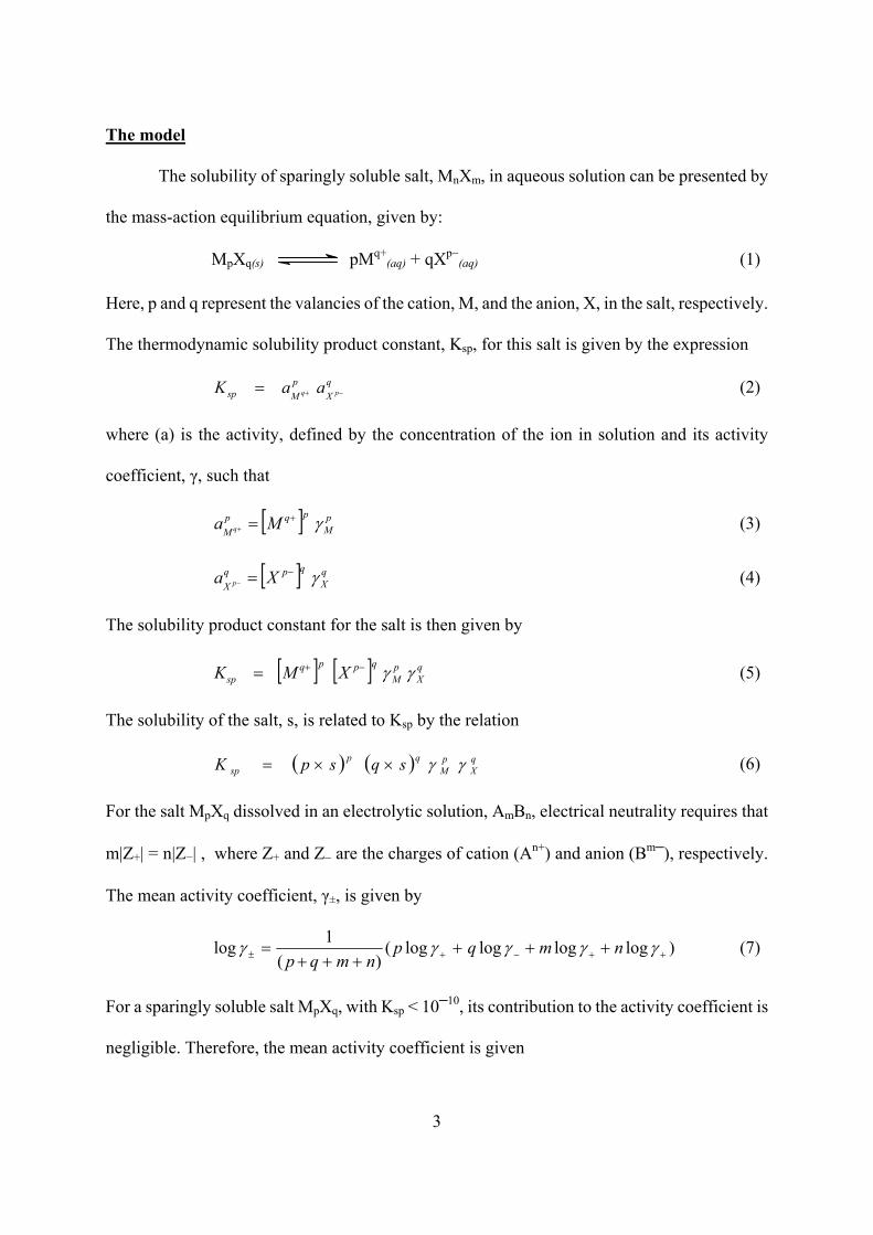
The model

The solubility of sparingly soluble salt, MnXm, in aqueous solution can be presented by

the mass-action equilibrium equation, given by:

MpXq(s) pMq+(aq) + qXp−

(aq) (1)

Here, p and q represent the valancies of the cation, M, and the anion, X, in the salt, respectively.

The thermodynamic solubility product constant, Ksp, for this salt is given by the expression

(2) qX

pMsp pq aaK −+=

where (a) is the activity, defined by the concentration of the ion in solution and its activity

coefficient, γ, such that

[ ] pM

pqpM Ma q γ+=+ (3)

[ ] qX

qpqX Xp γ−=−a (4)

The solubility product constant for the salt is then given by

[ ] [ ] qX

pM

qppqsp XMK γγ−+= (5)

The solubility of the salt, s, is related to Ksp by the relation

( ) ( ) qX

pM

qpsp sqspK γγ××= (6)

For the salt MpXq dissolved in an electrolytic solution, AmBn, electrical neutrality requires that

m|Z+| = n|Z−| , where Z+ and Z− are the charges of cation (An+) and anion (Bm─), respectively.

The mean activity coefficient, γ±, is given by

)loglogloglog()(

1++−+± +++

+++= γγγγγ nmqp

nmqplog (7)

For a sparingly soluble salt MpXq, with Ksp < 10─10, its contribution to the activity coefficient is

negligible. Therefore, the mean activity coefficient is given

4

)loglog()(

1−+± +

+= γγγ nm

nmlog (8)

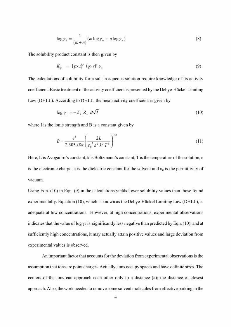
The solubility product constant is then given by

( ) ( ) ±××= γqpsp sqspK (9)

The calculations of solubility for a salt in aqueous solution require knowledge of its activity

coefficient. Basic treatment of the activity coefficient is presented by the Debye-Hückel Limiting

Law (DHLL). According to DHLL, the mean activity coefficient is given by

IBZZ −+± −=γogl (10)

where I is the ionic strength and B is a constant given by

2/1

33330

3 28303.2

=

TkL

xeB

εεπ (11)

Here, L is Avogadro’s constant, k is Boltzmann’s constant, T is the temperature of the solution, e

is the electronic charge, ε is the dielectric constant for the solvent and εo is the permittivity of

vacuum.

Using Eqn. (10) in Eqn. (9) in the calculations yields lower solubility values than those found

experimentally. Equation (10), which is known as the Debye-Hückel Limiting Law (DHLL), is

adequate at low concentrations. However, at high concentrations, experimental observations

indicates that the value of log γ± is significantly less negative than predicted by Eqn. (10), and at

sufficiently high concentrations, it may actually attain positive values and large deviation from

experimental values is observed.

An important factor that accounts for the deviation from experimental observations is the

assumption that ions are point charges. Actually, ions occupy spaces and have definite sizes. The

centers of the ions can approach each other only to a distance (a); the distance of closest

approach. Also, the work needed to remove some solvent molecules from effective parking in the

5

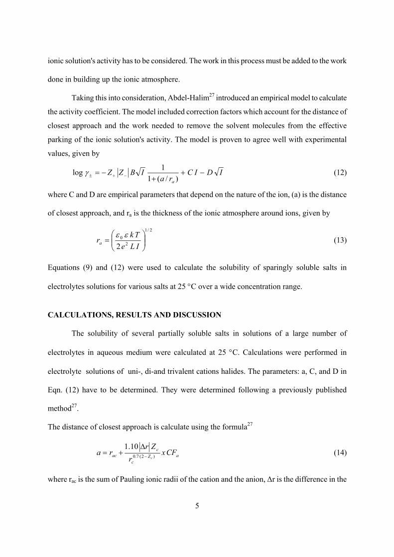
ionic solution's activity has to be considered. The work in this process must be added to the work

done in building up the ionic atmosphere.

Taking this into consideration, Abdel-Halim27 introduced an empirical model to calculate

the activity coefficient. The model included correction factors which account for the distance of

closest approach and the work needed to remove the solvent molecules from the effective

parking of the ionic solution's activity. The model is proven to agree well with experimental

values, given by

IDICra

IBZZa

−++

−= −+± )/(11log γ (12)

where C and D are empirical parameters that depend on the nature of the ion, (a) is the distance

of closest approach, and ra is the thickness of the ionic atmosphere around ions, given by

2/1

20

2

=

ILeTk

aεε

r (13)

Equations (9) and (12) were used to calculate the solubility of sparingly soluble salts in

electrolytes solutions for various salts at 25 °C over a wide concentration range.

CALCULATIONS, RESULTS AND DISCUSSION

The solubility of several partially soluble salts in solutions of a large number of

electrolytes in aqueous medium were calculated at 25 °C. Calculations were performed in

electrolyte solutions of uni-, di-and trivalent cations halides. The parameters: a, C, and D in

Eqn. (12) have to be determined. They were determined following a previously published

method27.

The distance of closest approach is calculate using the formula27

aZc

cac CFx

rZr

rc )2(7.0

10.1−

∆+=a (14)

where rac is the sum of Pauling ionic radii of the cation and the anion, ∆r is the difference in the

6

ionic radii of the ions, Zc is the charge of the cation, rc is the radius of the cation and CFa is a

correction factor that depends on the nature of the cation27.

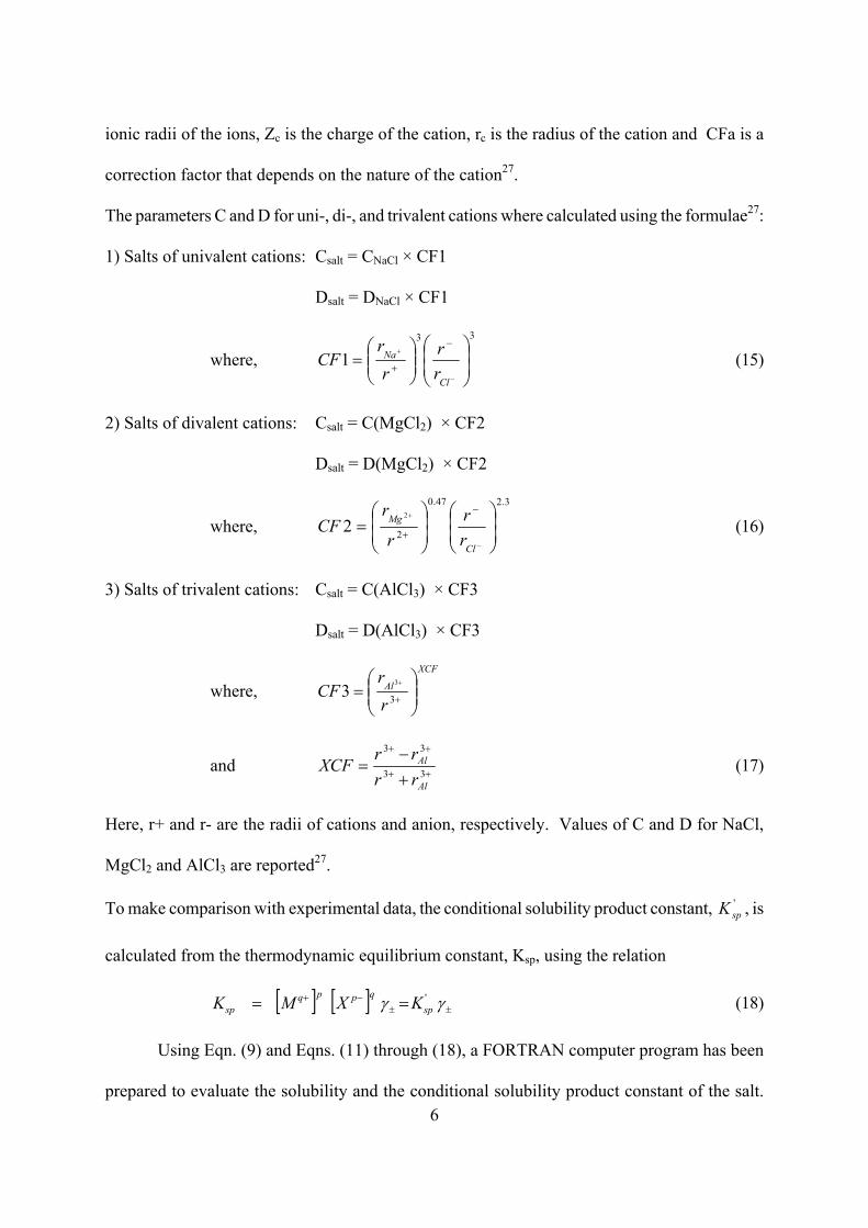
The parameters C and D for uni-, di-, and trivalent cations where calculated using the formulae27:

1) Salts of univalent cations: Csalt = CNaCl × CF1

Dsalt = DNaCl × CF1

where, 33

1

=

−

+−

+Cl

Na

rr

rr

CF (15)

2) Salts of divalent cations: Csalt = C(MgCl2) × CF2

Dsalt = D(MgCl2) × CF2

where, 3.247.0

2

2

2

=

−

+−

+Cl

Mg

rr

r

rCF (16)

3) Salts of trivalent cations: Csalt = C(AlCl3) × CF3

Dsalt = D(AlCl3) × CF3

where, XCF

Al

rr

CF

= +

+

3

33

and ++

++

+−

= 33

33

Al

Al

rrrr

XCF (17)

Here, r+ and r- are the radii of cations and anion, respectively. Values of C and D for NaCl,

MgCl2 and AlCl3 are reported27.

To make comparison with experimental data, the conditional solubility product constant, , is

calculated from the thermodynamic equilibrium constant, K

'spK

sp, using the relation

[ ] [ ] ±±−+ == γγ '

spqppq

sp KXMK (18)

Using Eqn. (9) and Eqns. (11) through (18), a FORTRAN computer program has been

prepared to evaluate the solubility and the conditional solubility product constant of the salt.

7

Calculations were performed for a large number of salts in several electrolytes aqueous

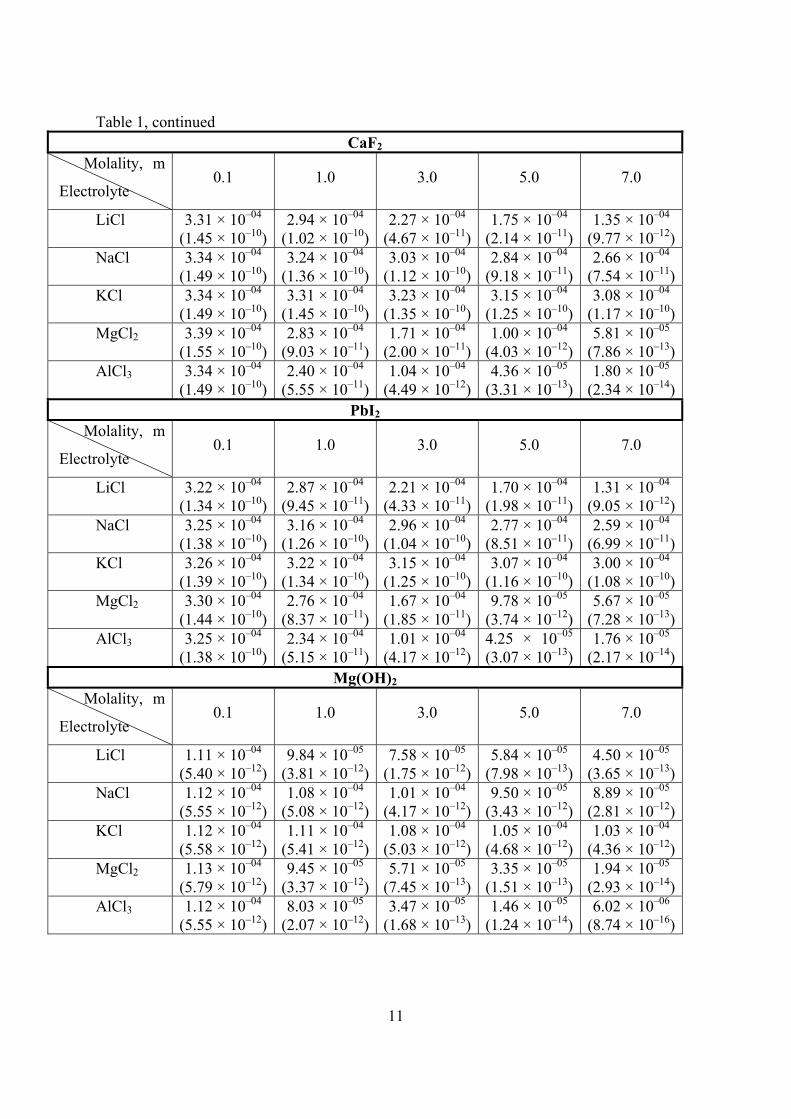
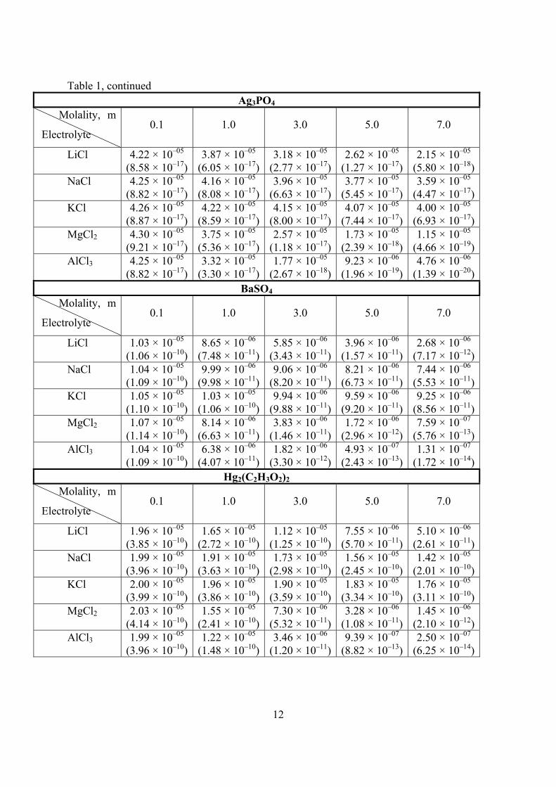
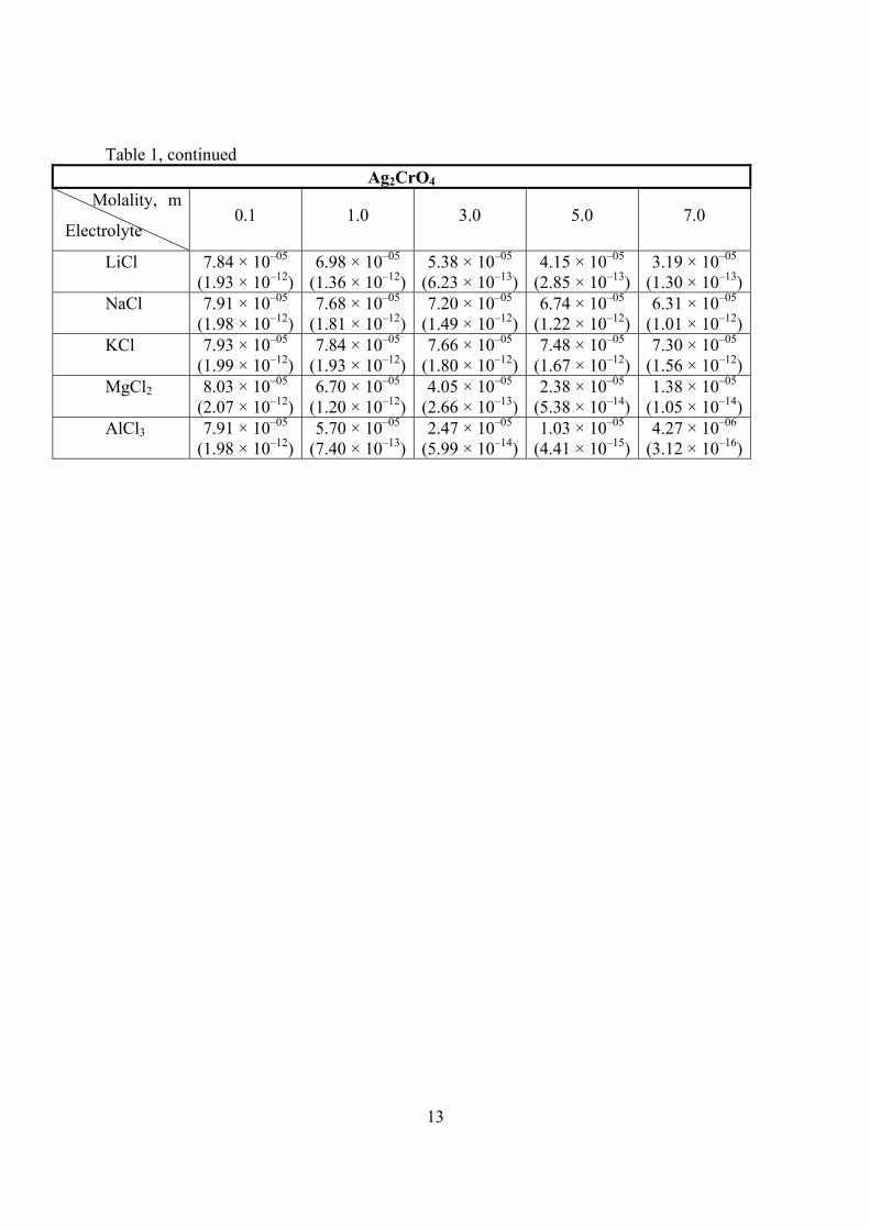
solutions, with wide range of concentrations, at 25 °C. Table 1 shows results of calculations for

ten selected salts in five different electrolytes solutions.

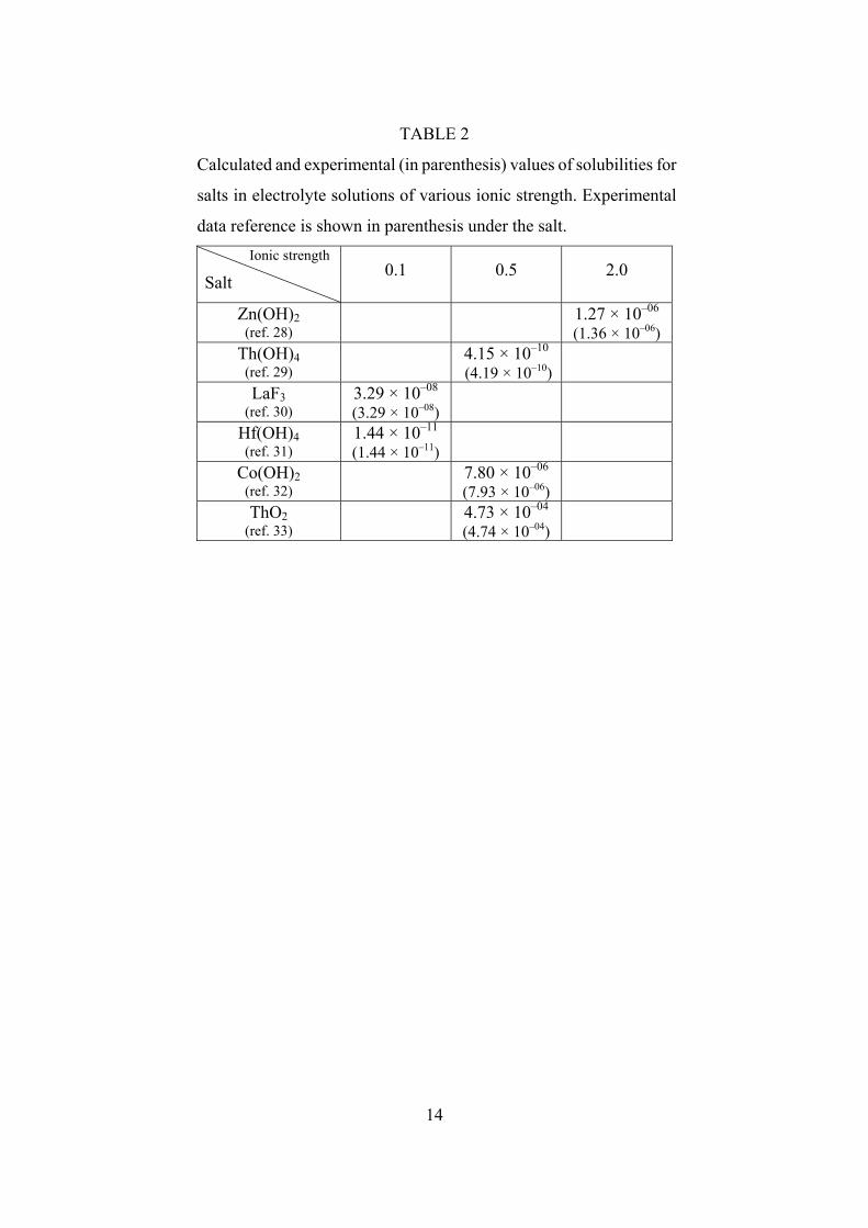
To check for the validity of the model in predict solubility at a given ionic strength, a

comparison is made between calculated and experimental solubility values. Table 2 shows

experimental solubilities, for some salts reported in literature, along with the calculated values.

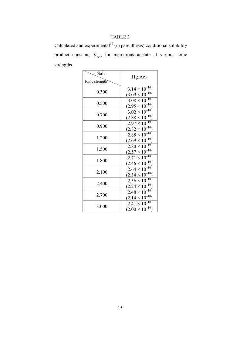
The agreement is extremely good for a wide range of ionic strength. For further check of the

validity of the model, the experimental values of the conditional solubility product constant for

mercurous acetate, a common salt extensively studied and reported in literature, are compared

with our calculated values. Table 3 shows a comparison between experimental and calculated

values at various ionic strengths. Taking this into consideration that the solubility product

constants are extremely difficult to obtain experimentally, because of the necessity to identify all

chemical species and processes present in the chemical system used to obtain their values. The

literature Ksp values, and hence solubility, may disagree widely, even by several orders of

magnitudes. Even though, the agreement is good and acceptable as shown in Table 3.

In summary, this new and simple model has been shown to be fairly effective in

calculating solubility and conditional solubility product constant for salt in electrolyte solutions.

A desktop calculator, or a simple computer program, can be used to perform the operations.

Though simple, the model has been demonstrated to be very accurate in predicting the solubility

and the solubility product for various salts over a wide concentration range of electrolyte

solutions.

8

1.

2.

3.

4.

5.

6.

7.

8.

9.

10.

11.

12.

13.

14.

15.

16.

17.

18.

REFERENCES

F. Hernandez-Luis, M. V. Vazquez and M. A. Esteso, J. Mol. Liq., 108, 283 (2003).

K. Fujiwara, H. Yamana, T. Fujii and H. Moriyama, Radiochim. Acta, 91, 345 (2003).

W. E. Waghorne, Monatshefte Chem., 134, 655 (2003).

K. Fujiwara, H. Yamana, T. Fujii and H. Moriyama, Radiochim. Acta, 90, 857 (2002).

R. Knopp, V. Neck and J. I. Kim, Radiochim. Acta, 86, 101 (1999).

X. Liu and F. J. Millero, Geochim. Cosmochim. Acta, 63, 3487 (1999).

A. Chhettry, Z. Wang, J. L. Fox, A. A. Baig, H. Zhuang and W. I. Higuchi, J. Coll. Inter.

Sci., 218, 47 (1999).

S. J. Friedfeld, S. He and M. B. Tomson, Langmuir, 14, 3698 (1998).

D. Chung, E. Kim, E. Lee and J. Yoo, J. Ind. Eng. Chem., 4, 277 (1998).

S. V. Mattigod, D. Rai, A. R. Felmy and L. Rao, J. Sol. Chem., 26, 391 (1997).

H. Fan, H. Jia, Y. Jiang and J. Pan, Chuan. Jishu Xuebao, 9, 33 (1996).

M. de Moraes, L. Pezza, C. B. Melios, M. Molina, R. Pezza, A. M. Peres, A. C. Villafranca

and J. Carloni, Ecletica Quimica, 21, 133 (1996).

S. Zhang, Z. He and K. Yang, Ziran Kexueban, 15, 82 (1992).

T. P. Dirkse, J. Electrochem. Soc., 133, 1656 (1986).

M. P. Menon, J. Chem. Eng. Data, 27, 81 (1982).

J. B. Macaskill and R. G. Bates, J. Phys. Chem., 81, 496 (1977).

J. R. Goates, A. G. Cole and E. L. Gray, J. Am. Chem. Soc., 73, 3596 (1951).

P. Debye and E.Hückel, Phys. Z., 24, 185 (1923).

9

19.

20.

21.

22.

23.

24.

25.

26.

27.

28.

29.

30.

31.

32.

33.

H. S. Harned and B. B. Owen, "Physical Chemistry of Electrolyte Solutions ", Reinhold,

New York, 1958.

R. A. Robinson and R.H. Stokes, "Electrolyte Solutions”, Butterworth, London, 1965.

F. Vaslow, "Water and Aqueous Solutions ", Wiley, New York, 1972.

H. P. Bennetto, Ann. Rev. Chem. Soc., 70, 223 (1973).

H. L. Friedman, C. V. Krishnan and C. Jolicoeur, Ann. N.Y. Acad. Sci., 204, 79 (1973).

R. H. Fowler, Proc. Camb. Phil. Soc., 22, 861 (1925).

J. G. Kirkwood and J. C. Poirier, J. Phys. Chem., 58, 591 (1954).

H. P. Bennetto and J. Spitzer, J. Am. Chem. Soc., 9, 2108 (1976).

H. M. Abdel-Halim, Asian J. Chem., 6, 370 (1994).

S. Xu and L. Xu, Ziran Kexueban, 4, 7 (2002).

V. Neck, R. Muller, M. Bouby, M. Altmaier, J. Rothe, M.A. Denecke and J.I. Kim,

Radiochimica Acta, 90, 485 (2002).

S. Shi, S.Yin and Y. Guo, Fenxi Ceshi Xuebao, 21, 44 (2002).

G. Gerefice, M. Draye, K. Noyes and K. Czerwinski, Materials Research Society

Symposium Proceedings (1999), 556 (Scientific Basis for Nuclear Waste Management

XXII), 1025.

V. E. Mironov, G. L. Pashkov, T. V. StuPko and Z.A. Pavlovskaya, Zhurnal

Neorganicheskoi Khimii, 40, 116 (1995).

E. Oesthols, J. Bruno and I. Grenthe, Geochimica et Cosmochimica Acta, 58, 613 (1994).

10

TABLE 1

Solubility and conditional solubility product constant (in parenthesis) of some sparingly soluble salts in aqueous electrolytes solutions of various concentrations at 25°C.

'spK

AgCl Molality, m

Electrolyte 0.1 1.0 3.0 5.0 7.0

LiCl 1.32 × 10–05 (1.73 × 10–10)

1.11 × 10–05 (1.22 × 10–10)

7.49 × 10–06 (5.61 × 10–11)

5.07 × 10–06 (2.57 × 10–11)

3.42 × 10–06 (1.17 × 10–11)

NaCl 1.34 × 10–05 (1.78 × 10–10)

1.28 × 10–05 (1.63 × 10–10)

1.16 × 10–05 (1.34 × 10–10)

1.05 × 10–05 (1.10 × 10–10)

9.51 × 10–06 (9.05 × 10–11)

KCl 1.34 × 10–05 (1.79 × 10–10)

1.32 × 10–05 (1.74 × 10–10)

1.27 × 10–05 (1.62 × 10–10)

1.23 × 10–05 (1.51 × 10–10)

1.18 × 10–05 (1.40 × 10–10)

MgCl2 1.36 × 10–05 (1.86 × 10–10)

1.04 × 10–05 (1.08 × 10–10)

4.89 × 10–06 (2.40 × 10–11)

2.20 × 10–06 (4.84 × 10–12)

9.71 × 10–07 (9.43 × 10–13)

AlCl3 1.34 × 10–05 (1.78 × 10–10)

8.16 × 10–06 (6.66 × 10–11)

2.32 × 10–06 (5.39 × 10–12)

3.26 × 10–07 (1.06 × 10–13)

1.68 × 10–07 (2.81 × 10–14)

Hg2Cl2 Molality, m

Electrolyte 0.1 1.0 3.0 5.0 7.0

LiCl 1.16 × 10–09 (1.35 × 10–18)

9.76 × 10–10 (9.52 × 10–19)

6.60 × 10–10 (4.36 × 10–19)

4.47 × 10–10 (2.00 × 10–19)

3.02 × 10–10 (9.12 × 10–20)

NaCl 1.18 × 10–09 (1.39 × 10–18)

1.13 × 10–09 (1.27 × 10–18)

1.02 × 10–09 (1.04 × 10–18)

9.26 × 10–10 (8.57 × 10–19)

8.39 × 10–10 (7.04 × 10–19)

KCl 1.18 × 10–09 (1.40 × 10–18)

1.16 × 10–09 (1.35 × 10–18)

1.12 × 10–09 (1.26 × 10–18)

1.08 × 10–09 (1.17 × 10–18)

1.04 × 10–09 (1.09 × 10–18)

MgCl2 1.20 × 10–09 (1.45 × 10–18)

1.09 × 10–09 (1.18 × 10–18)

4.32 × 10–10 (1.86 × 10–19)

1.94 × 10–10 (3.77 × 10–20)

8.56 × 10–11 (7.33 × 10–21)

AlCl3 1.18 × 10–09 (1.39 × 10–18)

7.20 × 10–10 (5.18 × 10–19)

2.05 × 10–10 (4.19 × 10–20)

5.56 × 10–11 (3.09 × 10–21)

1.48 × 10–11 (2.19 × 10–22)

MgCO3 Molality, m

Electrolyte 0.1 1.0 3.0 5.0 7.0

LiCl 2.56 × 10–03 (6.55 × 10–06)

2.15 × 10–03 (4.62 × 10–06)

1.46 × 10–03 (2.12 × 10–06)

9.84 × 10–04 (9.69 × 10–07)

6.66 × 10–04 (4.43 × 10–07)

NaCl 2.60 × 10–03 (6.74 × 10–06)

2.48 × 10–03 (6.17 × 10–06)

2.25 × 10–03 (5.07 × 10–06)

2.04 × 10–03 (4.16 × 10–06)

1.85 × 10–03 (3.42 × 10–06)

KCl 2.60 × 10–03 (6.78 × 10–06)

2.56 × 10–03 (6.56 × 10–06)

2.47 × 10–03 (6.11 × 10–06)

2.38 × 10–03 (5.69 × 10–06)

2.30 × 10–03 (5.29 × 10–06)

MgCl2 2.65 × 10–03 (7.03 × 10–06)

2.02 × 10–03 (4.10 × 10–06)

9.51 × 10–04 (9.05 × 10–07)

4.28 × 10–04 (1.83 × 10–07)

1.89 × 10–04 (3.56 × 10–08)

AlCl3 2.60 × 10–03 (6.74 × 10–06)

1.59 × 10–03 (2.52 × 10–06)

4.51 × 10–04 (2.04 × 10–07)

1.22 × 10–04 (1.50 × 10–08)

3.26 × 10–05 (1.06 × 10–09)

11

Table 1, continued CaF2

Molality, m

Electrolyte 0.1 1.0 3.0 5.0 7.0

LiCl 3.31 × 10–04 (1.45 × 10–10)

2.94 × 10–04 (1.02 × 10–10)

2.27 × 10–04 (4.67 × 10–11)

1.75 × 10–04 (2.14 × 10–11)

1.35 × 10–04 (9.77 × 10–12)

NaCl 3.34 × 10–04 (1.49 × 10–10)

3.24 × 10–04 (1.36 × 10–10)

3.03 × 10–04 (1.12 × 10–10)

2.84 × 10–04 (9.18 × 10–11)

2.66 × 10–04 (7.54 × 10–11)

KCl 3.34 × 10–04 (1.49 × 10–10)

3.31 × 10–04 (1.45 × 10–10)

3.23 × 10–04 (1.35 × 10–10)

3.15 × 10–04 (1.25 × 10–10)

3.08 × 10–04 (1.17 × 10–10)

MgCl2 3.39 × 10–04 (1.55 × 10–10)

2.83 × 10–04 (9.03 × 10–11)

1.71 × 10–04 (2.00 × 10–11)

1.00 × 10–04 (4.03 × 10–12)

5.81 × 10–05 (7.86 × 10–13)

AlCl3 3.34 × 10–04 (1.49 × 10–10)

2.40 × 10–04 (5.55 × 10–11)

1.04 × 10–04 (4.49 × 10–12)

4.36 × 10–05 (3.31 × 10–13)

1.80 × 10–05 (2.34 × 10–14)

PbI2 Molality, m

Electrolyte 0.1 1.0 3.0 5.0 7.0

LiCl 3.22 × 10–04 (1.34 × 10–10)

2.87 × 10–04 (9.45 × 10–11)

2.21 × 10–04 (4.33 × 10–11)

1.70 × 10–04 (1.98 × 10–11)

1.31 × 10–04 (9.05 × 10–12)

NaCl 3.25 × 10–04 (1.38 × 10–10)

3.16 × 10–04 (1.26 × 10–10)

2.96 × 10–04 (1.04 × 10–10)

2.77 × 10–04 (8.51 × 10–11)

2.59 × 10–04 (6.99 × 10–11)

KCl 3.26 × 10–04 (1.39 × 10–10)

3.22 × 10–04 (1.34 × 10–10)

3.15 × 10–04 (1.25 × 10–10)

3.07 × 10–04 (1.16 × 10–10)

3.00 × 10–04 (1.08 × 10–10)

MgCl2 3.30 × 10–04 (1.44 × 10–10)

2.76 × 10–04 (8.37 × 10–11)

1.67 × 10–04 (1.85 × 10–11)

9.78 × 10–05 (3.74 × 10–12)

5.67 × 10–05 (7.28 × 10–13)

AlCl3 3.25 × 10–04 (1.38 × 10–10)

2.34 × 10–04 (5.15 × 10–11)

1.01 × 10–04 (4.17 × 10–12)

4.25 × 10–05 (3.07 × 10–13)

1.76 × 10–05 (2.17 × 10–14)

Mg(OH)2 Molality, m

Electrolyte 0.1 1.0 3.0 5.0 7.0

LiCl 1.11 × 10–04 (5.40 × 10–12)

9.84 × 10–05 (3.81 × 10–12)

7.58 × 10–05 (1.75 × 10–12)

5.84 × 10–05 (7.98 × 10–13)

4.50 × 10–05 (3.65 × 10–13)

NaCl 1.12 × 10–04 (5.55 × 10–12)

1.08 × 10–04 (5.08 × 10–12)

1.01 × 10–04 (4.17 × 10–12)

9.50 × 10–05 (3.43 × 10–12)

8.89 × 10–05 (2.81 × 10–12)

KCl 1.12 × 10–04 (5.58 × 10–12)

1.11 × 10–04 (5.41 × 10–12)

1.08 × 10–04 (5.03 × 10–12)

1.05 × 10–04 (4.68 × 10–12)

1.03 × 10–04 (4.36 × 10–12)

MgCl2 1.13 × 10–04 (5.79 × 10–12)

9.45 × 10–05 (3.37 × 10–12)

5.71 × 10–05 (7.45 × 10–13)

3.35 × 10–05 (1.51 × 10–13)

1.94 × 10–05 (2.93 × 10–14)

AlCl3 1.12 × 10–04 (5.55 × 10–12)

8.03 × 10–05 (2.07 × 10–12)

3.47 × 10–05 (1.68 × 10–13)

1.46 × 10–05 (1.24 × 10–14)

6.02 × 10–06 (8.74 × 10–16)

12

Table 1, continued Ag3PO4

Molality, m

Electrolyte 0.1 1.0 3.0 5.0 7.0

LiCl 4.22 × 10–05 (8.58 × 10–17)

3.87 × 10–05 (6.05 × 10–17)

3.18 × 10–05 (2.77 × 10–17)

2.62 × 10–05 (1.27 × 10–17)

2.15 × 10–05 (5.80 × 10–18)

NaCl 4.25 × 10–05 (8.82 × 10–17)

4.16 × 10–05 (8.08 × 10–17)

3.96 × 10–05 (6.63 × 10–17)

3.77 × 10–05 (5.45 × 10–17)

3.59 × 10–05 (4.47 × 10–17)

KCl 4.26 × 10–05 (8.87 × 10–17)

4.22 × 10–05 (8.59 × 10–17)

4.15 × 10–05 (8.00 × 10–17)

4.07 × 10–05 (7.44 × 10–17)

4.00 × 10–05 (6.93 × 10–17)

MgCl2 4.30 × 10–05 (9.21 × 10–17)

3.75 × 10–05 (5.36 × 10–17)

2.57 × 10–05 (1.18 × 10–17)

1.73 × 10–05 (2.39 × 10–18)

1.15 × 10–05 (4.66 × 10–19)

AlCl3 4.25 × 10–05 (8.82 × 10–17)

3.32 × 10–05 (3.30 × 10–17)

1.77 × 10–05 (2.67 × 10–18)

9.23 × 10–06 (1.96 × 10–19)

4.76 × 10–06 (1.39 × 10–20)

BaSO4 Molality, m

Electrolyte 0.1 1.0 3.0 5.0 7.0

LiCl 1.03 × 10–05 (1.06 × 10–10)

8.65 × 10–06 (7.48 × 10–11)

5.85 × 10–06 (3.43 × 10–11)

3.96 × 10–06 (1.57 × 10–11)

2.68 × 10–06 (7.17 × 10–12)

NaCl 1.04 × 10–05 (1.09 × 10–10)

9.99 × 10–06 (9.98 × 10–11)

9.06 × 10–06 (8.20 × 10–11)

8.21 × 10–06 (6.73 × 10–11)

7.44 × 10–06 (5.53 × 10–11)

KCl 1.05 × 10–05 (1.10 × 10–10)

1.03 × 10–05 (1.06 × 10–10)

9.94 × 10–06 (9.88 × 10–11)

9.59 × 10–06 (9.20 × 10–11)

9.25 × 10–06 (8.56 × 10–11)

MgCl2 1.07 × 10–05 (1.14 × 10–10)

8.14 × 10–06 (6.63 × 10–11)

3.83 × 10–06 (1.46 × 10–11)

1.72 × 10–06 (2.96 × 10–12)

7.59 × 10–07 (5.76 × 10–13)

AlCl3 1.04 × 10–05 (1.09 × 10–10)

6.38 × 10–06 (4.07 × 10–11)

1.82 × 10–06 (3.30 × 10–12)

4.93 × 10–07 (2.43 × 10–13)

1.31 × 10–07 (1.72 × 10–14)

Hg2(C2H3O2)2 Molality, m

Electrolyte 0.1 1.0 3.0 5.0 7.0

LiCl 1.96 × 10–05 (3.85 × 10–10)

1.65 × 10–05 (2.72 × 10–10)

1.12 × 10–05 (1.25 × 10–10)

7.55 × 10–06 (5.70 × 10–11)

5.10 × 10–06 (2.61 × 10–11)

NaCl 1.99 × 10–05 (3.96 × 10–10)

1.91 × 10–05 (3.63 × 10–10)

1.73 × 10–05 (2.98 × 10–10)

1.56 × 10–05 (2.45 × 10–10)

1.42 × 10–05 (2.01 × 10–10)

KCl 2.00 × 10–05 (3.99 × 10–10)

1.96 × 10–05 (3.86 × 10–10)

1.90 × 10–05 (3.59 × 10–10)

1.83 × 10–05 (3.34 × 10–10)

1.76 × 10–05 (3.11 × 10–10)

MgCl2 2.03 × 10–05 (4.14 × 10–10)

1.55 × 10–05 (2.41 × 10–10)

7.30 × 10–06 (5.32 × 10–11)

3.28 × 10–06 (1.08 × 10–11)

1.45 × 10–06 (2.10 × 10–12)

AlCl3 1.99 × 10–05 (3.96 × 10–10)

1.22 × 10–05 (1.48 × 10–10)

3.46 × 10–06 (1.20 × 10–11)

9.39 × 10–07 (8.82 × 10–13)

2.50 × 10–07 (6.25 × 10–14)

13

Table 1, continued

Ag2CrO4 Molality, m

Electrolyte 0.1 1.0 3.0 5.0 7.0

LiCl 7.84 × 10–05 (1.93 × 10–12)

6.98 × 10–05 (1.36 × 10–12)

5.38 × 10–05 (6.23 × 10–13)

4.15 × 10–05 (2.85 × 10–13)

3.19 × 10–05 (1.30 × 10–13)

NaCl 7.91 × 10–05 (1.98 × 10–12)

7.68 × 10–05 (1.81 × 10–12)

7.20 × 10–05 (1.49 × 10–12)

6.74 × 10–05 (1.22 × 10–12)

6.31 × 10–05 (1.01 × 10–12)

KCl 7.93 × 10–05 (1.99 × 10–12)

7.84 × 10–05 (1.93 × 10–12)

7.66 × 10–05 (1.80 × 10–12)

7.48 × 10–05 (1.67 × 10–12)

7.30 × 10–05 (1.56 × 10–12)

MgCl2 8.03 × 10–05 (2.07 × 10–12)

6.70 × 10–05 (1.20 × 10–12)

4.05 × 10–05 (2.66 × 10–13)

2.38 × 10–05 (5.38 × 10–14)

1.38 × 10–05 (1.05 × 10–14)

AlCl3 7.91 × 10–05 (1.98 × 10–12)

5.70 × 10–05 (7.40 × 10–13)

2.47 × 10–05 (5.99 × 10–14)

1.03 × 10–05 (4.41 × 10–15)

4.27 × 10–06 (3.12 × 10–16)

14

TABLE 2

Calculated and experimental (in parenthesis) values of solubilities for

salts in electrolyte solutions of various ionic strength. Experimental

data reference is shown in parenthesis under the salt. Ionic strength

Salt 0.1 0.5 2.0

Zn(OH)2 (ref. 28)

1.27 × 10–06 (1.36 × 10–06)

Th(OH)4 (ref. 29)

4.15 × 10–10 (4.19 × 10–10)

LaF3 (ref. 30)

3.29 × 10–08 (3.29 × 10–08)

Hf(OH)4 (ref. 31)

1.44 × 10–11 (1.44 × 10–11)

Co(OH)2 (ref. 32)

7.80 × 10–06 (7.93 × 10–06)

ThO2 (ref. 33)

4.73 × 10–04 (4.74 × 10–04)

15

TABLE 3

Calculated and experimental12 (in parenthesis) conditional solubility

product constant, , for mercurous acetate at various ionic

strengths.

'spK

Salt Ionic strength

Hg2Ac2

0.300 3.14 × 10–10 (3.09 × 10–10)

0.500 3.08 × 10–10 (2.95 × 10–10)

0.700 3.02 × 10–10 (2.88 × 10–10)

0.900 2.97 × 10–10 (2.82 × 10–10)

1.200 2.88 × 10–10 (2.69 × 10–10)

1.500 2.80 × 10–10 (2.57 × 10–10)

1.800 2.71 × 10–10 (2.46 × 10–10)

2.100 2.64 × 10–10 (2.34 × 10–10)

2.400 2.56 × 10–10 (2.24 × 10–10)

2.700 2.48 × 10–10 (2.14 × 10–10)

3.000 2.41 × 10–10 (2.00 × 10–10)