A Model of Soviet-Type Economic Planning

A Model of Soviet-Type Economic

Planning

By MICHAEL MANOVE*

Each year, planning agencies in the Soviet Union construct an annual economic plan for the calendar year that follows. The annual plan is an important element in the Soviet schema for achieving long-term economic growth. Goals of less detailed long-range plans must be considered in the design of the annual plan. Furthermore, the plan is supposed to ex- pose and remedy weak links in the economic structure. But the most important and obvious purpose of the annual plan is to ensure that the economy will function in a reasonable way from day to day.1

The material supply plan is a major component of the Soviet-type annual plan. It specifies aggregate output targets and other production indices from which output targets and certain production indices for individual productive units are derived. The traditional procedure for constructing the material supply plan is very complicated and involves a large planning bureaucracy. In fact, it is difficult to determine from the descriptive literature how rational the planning procedure is, or even how different elements of the procedure fit

together.2 In this paper, an attempt is made to establish a theoretical under- pinning for this traditional Soviet-type planning procedure.3 In particular, we try to analyze how, in theory, a planning procedure of this type can produce a consistent plan, i.e., a plan in which the supply and demand for each commodity is balanced.4 In order to simplify our task, we shall not consider the Soviet planning system itself. Rather, we shall concentrate our analytical efforts on a more transparent, though not dissimilar, planning system- namely, that of the Autonomous Soviet Republic of Morozhenoe. The planning procedures of this republic oblige us by in- corporating only the most basic elements of traditional Soviet-type systems.

I. Characteristics of an Annual Plan

Morozhenoe, incorporated as an Au- tonomous Republic of the Russian Soviet Federated Socialist Republic shortly after World War II, is the only Soviet republic that has been completely autonomous in the economic sphere. Even more surprisingly, despite the fact that Moroz- henoe has a smaller gross product than

* Assistant professor of economics, University of Michigan. I am indebted to Maria Augustinovics, Michael Bruno, Evsey D. Domar, Richard S. Eckaus, Duncan K. Foley, Martin L. Weitzman, and a referee for their extremely helpful comments and suggestions at various stages of this work. I wish to acknowledge financial support and encouragement from the Com- parative Economics Program of the University of Mich- igan.

1 According to G. Sorokin (p. 225), the long-term plan outlines ways of achieving the main tasks of economic development, the five-year plan elaborates construction and operational plans in greater detail, and the annual plan itemizes the five-year program and facilitates economic management. The annual plan is legally binding.

2 The most extensive description by a western scholar of Soviet material-supply planning is contained in the unpublished doctoral dissertation of Herbert Levine (1961). A condensation of the dissertation appears in his 1959 paper. I. A. Evenko (pp. 72-88) is another source of general descriptive material. For a description of the Polish procedure, see J. M. Montias (1962, pp. 6-32, 76-114).

3 An excellent survey of possible theoretical approaches is contained in Montias (1959).

4 For general information on the consistency of Soviet plans, see Michael Ellman. Montias (Oct. 1962) dis- cusses the possibility of utilizing the decomposability of the A-matrix to produce consistent plans.

390

manove

Text Box

The American Economic Review, Vol. 61, No. 3, Part 1 (Jun., 1971), pp. 390-406

MANOVE: SOVIET-TYPE PLANNING 391

even Darien, Connecticut, this little republic is virtually self-sufficient and en- gages in little external trade.

Wishing to embark on a program of rapid industrialization, the Morozhenoens decided to construct a "command economy," of which an annual plan of material supply was to be an integral part. Because the system envisioned was to be basically non-market, the annual plan would have to serve as the main guide for the producing units of the economy in their day-to- day operations. The system for constructing such short-term material supply plans, it was decided, ought to have the following characteristics:

1) The authorities specify net output levels of final goods (including capital goods and planned inventory accumula- tions).

2) The system yields a plan which determines, at the very least, a set of output targets for each producing unit.

3) The system yields a plan which is internally consistent. For each output target specified by the plan, sufficient quantities of the necessary inputs must be provided.5

4) The system yields a plan which is reasonably efficient in the short run. To the extent permitted by long-term constraints, existing resources and factors of production should be put to full and reasonable use. If the necessary labor is available, a short-term plan ought to set output targets at levels which utilize the full capacities of most producing units. The Morozhenoens did realize, however, that the scope of an annual plan is too limited to deal with questions of efficiency involv- ing the allocation of capital or major shifts in technology.

II. The Input-Output Planning Procedure

The Morozhenoens have had a long

standing aversion to Russian bureaucratic planning methods. In 1947, risking Mos- cow's ire, they invited a well-known Amer- ican economist from a major New England academic institution to design for them a simple, non-bureaucratic material supply planning system. They stipulated that the system have the previously discussed characteristics. The American advised the use of the following input-output procedure.

Let yj be the gross output target for commodity j, dj the final demand for commodity j, and aij the input of commodity i required per unit output of commodity j (a fixed-proportions production function is assumed), and let Y, D, and A denote the corresponding vectors and matrix, respectively. Suppose that A and D are known. To determine a consistent set of gross output targets, gross supplies are equated with gross demand :6

(1) Y = AY+ D

Solving for Y, we obtain

(2) Y = (I- A)-ID

where I is the identity matrix. The vector Y may also be given inductively, as in the following:

(3) Y = A Y(i1) + D

where Y(i) approaches Y as i gets large. Equation (3) specifies what we shall call

a "supply-demand iteration"; it sets a new output (supply) vector equal to the demand vector associated with a previous output vector. To use (3), one starts out by specifying a tentative gross output vector, say Y(o). The right-hand side of (3) yields the demand vector associated with

I This is only one sense in which a plan may be said to be consistent. Richard Stone provides a fairly complete summary of the concept of consistency in planning.

6 In this paper, the terms "output" and "supply" are used interchangeably. Imports and planned decreases in inventory stocks are considered to be negative sum- mands of final demand. The demand for an intermediate good is completely determined by the output targets and the fixed-proportions production functions and is assumed to be strictly independent of price.

392 THE AMERICAN ECONOMIC REVIEW

the production of Y(o); namely, A Y(o)+D. A new tentative output vector Y(j) would then be defined as equal to this demand vector. Equation (3) would be applied re- peatedly, yielding Y(2), Y(3), and so on.

If any given output vector Y(j) were produced, then the corresponding demand vector would be A Y(i)+D. Let E(i) be defined as the supply-demand imbalance associated with the production of Y(,), that is, the difference between the supply Y(i), and the demand A Y(i)+D. Then, the imbalance associated with Y(j) is given by

E (j) = A iE (O)

Since A is productive,7 we know that Ai approaches 0 as the exponent i gets large. It follows that with succeeding supply- demand iterations E(i) also approaches 0 and that Y(j) goes to Y. (How fast does the supply-demand imbalance approach O? A trial with a 38-sector A -matrix for the USSR and with E(o) proportional to gross output, revealed that in general, each iteration cut the supply-demand imbalance roughly in half.)8

If the demand for final products, D, and the input norms, A, are known to a central planning agency, the agency could grind out Y with a computer in a relatively short period of time using either (2) or (3). It would remain to disaggregate the gross output targets with respect to individual enterprises. In Morozhenoe, however, because of the relatively small number of enterprises, this would present few difficulties.

T he input-output procedure is extremely attractive because of its simplicity and because plans produced by it are perfectly consistent. And while the above planning method does not imply short-run eflici- ency (which depends on the values of A and D), it is not incompatible with it. Un- fortunately, the input-output procedure could not be successfully implemented in Morozhenoe.

The principal difficulty with the scheme was that all information on A and D had to be known by the center in order to be used. The relevant information had to be obtained in great detail at the local level and then summed up for the entire economy, a task which overwhelmed Moroz- henoen information processing facilities. Even for this small 100t-good economy, there are a total of 1,001,000 entries in A and D, of which roughly 200,000 are non- zero.9 And since the amount of data to be

7 A technology matrix A is said to be productive if a positive vector of net outputs is producible; i.e., A is productive if, and only if, there exists Y such that Y-A Y>0 (in every component). It can be shown that A is productive if, and only if, (J-A)-' exists and is nonnegative.

8 A 38-sector A -matrix and a vector Y of gross outputs for the Soviet Union were obtained from V. Treml (1966). Starting with supply-demand imbalances proportional sec.tor-by-sector to gross outputs, successive supply-demand iterations (3)-or, equivalently, successive multiplications of the imbalance vector by the A -matrix-reduced the ruble value of the supply-demand imbalances by an average of 51.0 percent per iteration. In the sector with the smallest average reduction, the imbalance was reduced by 28.4 percent per iteration. Had we assumed that the imbalances in different sectors had differing signs, the reductions would have been considerably greater. (Note: successive iterations do not reduce the imbalance in a given sector by a constant percentage; the above figures are arithmetic averages, with each percentage reduction weighted by the size of the imbalance before the iteration.)

It is unlikely that the degree of aggregation of the A -matrix and the imbalance vector would have a signif- icant effect on the rate at which multiplication of the

imbalance vector by the A -matrix reduces that vector. The above experiment was repeated with a 17-sector version of Treml's matrix, and the results were virtually unchanget. Indeed, if we assume that the A-matrix was derived from an input-output table, and if the original imbalance vector is proportional to the gross output vector given in that table, then it can be shown that the percentage change in total value of the imbalances as a result of multiplication by the A-matrix is independlent of the degree of aggregation.

9 A crude estimate. In Eidel'man (p. 237), it is reported that 4,754 non-zero entries were contained in 83-sector Soviet 1959 A -matrix. Assuming that the number of non-zero entries in an A-matrix is greater than proportional to the dimension of the matrix and less than proportional to the number of entries in the


compiled grows more than proportionally to the number of commodities produced, the difficulty of this task increased rapidly as the economy grew and became more com- plex. 10

By 1953, trial use of the input-output planning procedure was discontinued. The stock of unwanted inventories equaled almost two-thirds the size of the annual gross national product, and shortages abounded. The leading Morozhenoen economists realized that this situation resulted not from any error internal to the planning procedure, but rather from the use of in- correct values in the A-matrix and in the final demand vector D. Some economists argued that the techniques of information gathering should be improved and that the input-output planning system be retained. But they were overruled by the authorities who insisted that the planning system be scrapped in favor of a new system that requires much less information in order to function. The Morozhenoen government set up an emergency committee to draw up an annual planning procedure based on Russian. practices at the time. On October 20, 1953, this new procedure was formally adopted.

III. The Soviet-Type Planning Procedure in Morozhenoe

The Soviet-type planning procedure depends on the existence of a large planning bureaucracy, both at the central and at the enterprise levels. All commodities are placed in either of two categories: centrally planned commodities and locally planned commodities. Information on locally planned commodities is processed

entirely at the enterprise level, while information pertaining to centrally planned commodities is passed back and forth between the central planning agency and the enterprises.

In Soviet Morozhenoe, the central planning agency is known as Gosplan. Gosplan has a series of departments organized along industrial lines. Each centrally planned commodity is assigned to two of these departments: a so-called summary department, and an industrial department. The summary departments are responsible for processing information dealing with demand and distribution of commodities, while industrial departments deal with the supply of commodities from production and other sources. Gosplan also contains statistical departments and final-demand departments. How the various departments of Gosplan interact with each other and with local planning agencies is described on the following pages.

Conceptually speaking, the Soviet-type planning procedure may be thought of as a series of iterations. These iterations are of three types, all of them variants of the basic supply-demand iteration described by equation (3). One of these, the "retrospective iteration," may be used by local planning agencies in determining output targets for locally planned commodities, and by central planning agencies in determining output targets for centrally planned commodities. The other two, the "external iterations" and the "internal iterations," require certain centrally processed information, and, consequently, may be used to adjust the output targets of only centrally planned commodities. In Morozhenoe, the process of drawing up an annual plan spans a one-year period.

The principal steps of the annual planning procedure are outlined below (see, also, Figure 1) and a mathematical representation for the procedure is presented.

Let n denote the number of commodities

matrix, a guess of 200,000 as the number of non-zero elements in the 1000.xiOO Morozhenoen A-matrix was derived by taking a geometric average of 4754xlO00/83 and 4754x(1000/83)2.

10 The difficulties of applying input-output methods to Soviet planning are outlined by A. Dorovskikh (pp. 38-39).


CENTRAL PLANNING AGENCY

REVISED ESTIMATED OUTPUT TOTAL TARGETS DEMAND

~~~~~..... ............... . _

RETROSPECTIVE DEM : FN

ITERATION INTERNAL TDM ITERATION ~~~I TERA TION

INPUT

LOCAL PLANNING AGENCIES REQUIREMENTS

RETROSPECTIVE i ITERATION PRELIMINARY

OUTPUT OFFICIAL TARGETS FOR OUTPUT TARGETS CENTRALLY A FOR CENTRALLY PLANNED PLANNED

OFFICIAL CMOIE COMMODITIES OUTPUT TARGETS FOR LOCALLY / I PLANNED Y COMMODITIES *

EXTERNAL

ENTERPRISES ENTERPRISES I TERA TION

I i t I * 12, .l | I~~~~~~~~~~~~~~I j JI I

ESTIMATED REQUIREMENTS FOR CENTRALLY PLANNED INPUTS

FIGURE 1-SOVIET-TYPE MATERIAL-SUPPLY PLANNING PROCEDURE: A STYLIZED VERSION

being produced. All of the vectors defined below are n-dimensional; the ith component of a vector always pertains to commodity i. If the vector is subscripted, the subscript refers to the year for which the vector is defined. Each commodity is produced by many enterprises. The word "aggregate" is used to indicate a nation- wide total pertaining to a given commodity, and not the combining of different commodities. A list of symbols used appears in the Appendix.

Step 1: Specification of preliminary aggregate output targets: a retrospective iteration (January-March)."

For each centrally planned commodity, the center sets a preliminary aggregate output target by adding an exogenously determined increment in gross output to the previous year's aggregate demand.'2

The preliminary aggregate output targets (control figures) are then used to assign output targets to individual enterprises.

No preliminary aggregate output targets are set for locallv planned commodities. Instead, a preliminary output target is set independently for each enterprise producing a given commodity, by adding an exogenously determined increment in production to the demand for the commodity on the enterprise (i.e., the orders placed with the enterprise) during the previous year. The reader should note that while a preliminary output target is not set, or known, for a locally planned product, such a target does in fact exist-namely, the sum of all of the enterprise output targets for the product.

For both centrally and locally planned

11 The time periods given here are similar to those for the Soviet Union as reported in Evenko, (p. 84).

12 It is assumed that in cases where actual requirements for centrally planned inputs differ from planned

allotments, producers will ask the center to make appropriate adjustments in the allotments. These requests for adjustments enable the center to calculate actual aggregate demand for centrally planned products after the fact.


commodities, preliminary output targets (potential supplies) are based on actual demands of the previous year. Thus the designation retrospective iteration.

Let Y, be the vector of preliminary aggregate output targets for year t. Then, in accordance with the above specifications, Yt is given by the vector equation

=t = t-1 + Qt

where Qt is a vector of exogenously determined increments (or decrements, if negative) to aggregate outputs,'3 and Xt is the vector of aggregate demands. For analytical purposes, however, we shall allow the possibility of omitting the retrospective iteration for some commodities, in which case the previous year's output would be substituted in the above equation for the previous year's demand. Therefore we amend the equation to

(4) Yt = QXt_l + (I -Q) )t- + Qt

where Yt is the vector of aggregate outputs, Q is a diagonal matrix whose ith entry is equal to 1 if commodity i is to be iterated retrospectively, and 0 otherwise. All quantities indicated in (4) are aggregate quantities.

Equation (4) is valid for both centrally and locally planned commodities, but for a different reason in each of the two cases. It is true for centrally planned commodities because the right-hand side of the equation .actually describes the way the center sets preliminary aggregate output targets. Equation (4) is valid for locally planned commodities, because an equation analogous to (4) but in terms of non- aggregate quantities, defines each enterprise target. Summing all of the non- aggregate equations pertaining to a particular locally planned commodity yields

the relationship for aggregate quantities expressed by (4).

Step 2: Computation of tentative demands (April-June). The vector X, of tentative aggregate demands induced by the preliminary output targets Yt, is given by

(5) Xt = A ft + Dt

where Dt is the vector of planned final demands. Gosplan, however, cannot use this equation to compute the tentative demands, since it does not necessarily know the value of the A-matrix or the values of Yt and Dt pertaining to locally planned commodities. Instead, Gosplan calculates aggregate demands for centrally planned products only. The following procedure is used:

All enterprises submit estimates of the quantities of all centrally planned commodities they plan to use as inputs.14 In making these estimates, each enterprise assumes its output will equal its preliminary output target. The estimates of required inputs are aggregated and for- warded to Gosplan. At the same time, final demands for centrally planned products are set by final demand departments of Gosplan, which, at its discretion, may be guided by consumers' and investors' de- sires.15 Each summary department of Gosplan then determines estimates of aggregate demands for the centrally planned products assigned to it by adding the demand for each product as an input to the respective final demand.

Step 3: Revision of the preliminary output targets for centrally planned commodities: an external iteration (July).

At this point, the summary departments of Gosplan consult with the corresponding industrial departments. If the tentative

13 The centrally planned components of Q, are set explicitly by Gosplan; the locally planned components are the sums of exogenous changes made by local planning agencies.

1F For a description of this process in the USSR, see Levine (1959, pp. 156-59).

15 The planning of consumption is treated at length by Phillip '5'eitzman.


demands do not equal the tentative supplies-and they surely will not-then the demand and supply figures must be recon- ciled. In order to effect this reconciliation, Gosplan uses the material balance, an accounting device in which all supplies of a commodity, on the one hand, and all demands for the commodity, on the other, are tabulated. In most Socialist countries, the process of adjusting supplies and demands in order to bring about a balance is extremely complicated and draws heavily on the experience and intuition of the planners. In Soviet Morozhenoe, however, only one basic aspect of the process is used. The preliminary output targets for centrally planned commodities are reset to equal the respective aggregate demand estimates. Thus a new tentative aggregate gross output target is formulated for each centrally planned commodity.

The output targets for locally planned commodities remain unchanged.

Let Yt(o) be the revised vector of aggregate gross output targets. It follows from the above that Yt(o) will equal Xt in centrally planned components and Yt in locally planned components. These relationships can be expressed as one equation:

(6) Yt(0) = rXt + (i - r) Yt

where r is a diagonal matrix with entries pertaining to centrally planned commodities set equal to 1, and entries pertaining to locally planned commodities set equal to 0.

As far as centrally planned commodities are concerned, Steps 2 and 3 have the same result as one supply-demand iteration (3) of the input-output procedure, in that the demands generated by the preliminary output targets become new output targets. With the input-output procedure, however, the center must calculate the demands for inputs from its knowledge of production functions (the A-matrix), while in Step 2 of the Soviet-type procedure, the

center (Gosplan) allows the producing units (enterprises) to estimate their own input demands. Because part of the demands are estimated outside of the center, Step 3 is referred to as an external iteration.

Step 4: Further revisions of tentative output targets for centrally planned commodities :16 internal iterations (August).

In principle, the internal iteration is a straightforward process. Whenever the tentative aggregate output targets for centrally planned commodities are revised, the tentative input requirements of the producers of centrally planned commodities will change. When an industrial department of Gosplan changes (or is advised of a change in) output targets of commodities under its purview, it may advise appropriate summary departments of resulting changes in the input requirements of the industry, provided, of course, that the information necessary to compute the changes in requirements is available. After the summary departments receive notifica- tion of changes in input requirements from all of the industrial departments, the summary departments may proceed to calculate a revised set of aggregate demands for the centrally planned commodities. The summary departments may then consult with the corresponding industrial departments, so that the latter can set new aggregate output targets equal to these revised aggregate demands.

Let Yt(j) denote the tentative aggregate output targets after i internal iterations. Then we may represent an internal iteration by

(7) Yt(i) = rXt(j_l) + (I - r) Yt

where Xt(i), the vector of tentative ag-

16 That a realistic model of Soviet-type planning ought to include this step was suggested by Martin Weitzman, Yale University, and by Maria Augustinovics, Head, Division of Long-term Planning, National Planning Institute, Budapest, Hungary.


gregate demands after i internal iterations, is given by

(8) Xt(j) = A Yt(i) + Dt

The internal iteration also yields results like those of the supply-demand iteration (3), except that in this case, only the output targets of centrally planned commodities are revised. The name internal iteration derives from the fact that all computation is performed within Gosplan, itself. In order for the internal iteration to be carried out, the industrial departments must have certain information about input usage in the production of commodities under their purview. In particular, they must know the specific coefficients in the A-matrix which yield the quantities of centrally planned inputs needed to produce these commodities.

Step 4 consists of a number of internal iterations, a number bounded by time, cost and information constraints on Gos- plan. Because of these constraints, some of these internal iterations may have to be partial,17 or all internal iterations may even be omitted.

At this point, the reader may be wonder- ing why an external iteration is necessary given that subsequent iterations may be internal. The explanation lies in the fact that the first calculation of tentative aggregate demands for centrally planned commodities requires more information than subsequent calculations do. The first calculation requires information on centrally planned inputs used to produce all commodities, both centrally and locally planned. But, because the tentative out-

put targets for centrally planned commodities are the only ones that change in the iterations, subsequent calculations of the tentative aggregate demands require information pertaining only to the use of centrally planned inputs in the production of centrally planned commodities. Fur- thermore, the center may be able to obtain much of the information needed to execute internal iterations as a by-product of the external iteration.

Step 5: Specification of the official output targets (September-December).

The most recently derived tentative aggregate gross output targets for centrally planned commodities become official targets after approval by various government bodies. These targets are then disaggre- gated and assigned to the individual enterprises producing centrally planned commodities. Official output targets for locally planned goods are the same as the preliminary targets set in Step 1.

If n internal iterations were carried out, the official output targets Yt are given by

(9) =t = Yt (n)

It is clear that the Soviet-type planning procedure is less demanding with regard to information gathering than is the input- output procedure. The input-output procedure required the center to know all of the elements of the A-matrix, to calculate total output and demand for each commodity, and to know or set total final demand for each commodity. The Soviet- type procedure, however, requires only that the center calculates total output and demand for centrally planned commodities and that it knows or sets final demand for centrally planned commodities. If internal iterations are omitted, knowledge of the A- matrix by the center is not required. How- ever, if the center does know coefficients pertaining to the use of centrally planned inputs in the production of centrally planned commodities, it may use them to

17 For the sake of mathematical simplicity in analyz- ing the model, I have assumed that an internal iteration involves all centrally planned commodities. A more general model would allow internal iterations to be performed for any subset of the centrally planned commodities. This would permit the center to carry out partial internal iterations which would require the knowledge of technical coefficients only for those commodities involved.


carry out internal iterations, thereby in- creasing the degree of consistency of the plan-as we shall see.

As the Soviet-type procedure was being established in Morozhenoe, many economists there predicted that plans produced by the procedure would be subject to catastrophic failure. It was agreed that the system does allow (but does not require) the authorities to set the level of final demand for a commodity, and does yield output targets for each producing unit. There was some concern about short- run economic efficiency. But the major cause of skepticism centered around the question of consistency.18 Why, it was asked, should the planned supply of a commodity equal the resulting demand for it? For one thing, only about one-third of all commodities were to be centrally planned. Considering the fact that current output targets for locally planned goods are not directly coordinated with the current output targets for centrally planned goods, what assurances are there that the supplies of locally planned goods required as inputs throughout the economy would be available? The usefulness of the external and internal iterations seemed doubtful for two reasons: the planners would have time and funds available for at most a few iterations, and only centrally planned output targets were being revised. It was suggested that the abolition of all central planning would be preferable to these halfway measures.

Between 1954 and 1956, the chaotic state of the Morozhenoen economy seemed to bear out the pessimism of the economists. But, surprisingly, the plan of 1957 turned out to be almost consistent. The

supply and demand for each centrally planned product differed at most by a few percentage points, and the supply and demand for each locally planned product differed by no more than about 5 percent. And this, despite the fact that internal iterations had been entirely omitted from the planning procedure for economy reasons. Results in later years were just as good. An analysis of the model suggests an explanation.

IV. An Analysis of the Soviet- Type Procedure

It is assumed that the relationship between actual outputs Yt, demands for the outputs Xt, and final demands Dt, is given by

(10) Xt = A Yt + Dt The vector of supply-demand imbal-

ances Et is given by

(11) Et= Yt-Xt

For the purposes of this analysis, we make the simplifying assumption that the planned output targets are always exactly fulfilled, i.e.,

(12) Yt = Ft

This implies that Et will be generated only by the inconsistencies in the plan.

The assumption that output targets are precisely met also implies that the supply- demand imbalances represented by Et manifest themselves as economic occur- rences with little or no secondary effects: perhaps as unplanned changes in the levels of consumption,19 in the levels of exports or imports, or, under certain circum- stances, in the size of inventory stocks. In

18 Problems of feasibility are avoided by assuming that the Morozhenoens always choose final demands so as to fall within the production possibility curve. Thus if a plan is internally consistent, it is also feasible. The problem of feasibility is treated more realistically in the author's doctoral dissertation.

19 Of course, unplanned (or any other) changes in the level of consumption will have important secondary effects outside the sphere of production. And if the changes are large enough, or if the population is close to the subsistence level, changes in consumption may effect labor, and consequently, production.


other words, the entire error falls on final demand. Although these assumptions are unrealistic (even in Morozhenoe), they serve to isolate the direct effects of incon- sistent plans from the secondary effects, which depend to a large extent on how the economic administration handles the shortages or surpluses that arise from the inconsistencies.

The vector Et tells the complete story as far as consistency of the plan is concerned. If Et=O, then the plan is perfectly consistent, if the components of Et are large (+ or -), then large surpluses and/or shortages are indicated. We attempt to throw some light on the genesis of Et in the Morozhenoen planning procedure by solving the mathematical representation of that procedure. For simplicity, we shall assume that no internal iterations (Step 4) are carried out. Under this circum- stance, equations (6)-(9) and (12) reduce to

(13) Yt = rXt + (I - F) Yt

The model of the planning procedure with internal iterations is analyzed in the Ap- pendix.

Equations (4), (5), (10), (tl), and (13) can be solved simultaneously for the supply-demand imbalance ET realized in a given year T. If, as we may do without loss of generality, we set Yo=Do=O, the solution is as follows:

T

(14) ET = E (r[lQ[lI)Ttr[llLt t=1

where

(15) Lt = Qt- (AQt + A Dt)

(16) F[l=I- (I- A)F

and

(17) Q[11 = I -(I -A)Q

and where ADt =Dt-Dt-1. Equation (14) has a helpful heuristic

interpretation. Note that (14) gives the supply-demand imbalance ET for year T as a weighted sum of Lt's. What does Lt represent? Recalling that Qt is the exogenously determined increment in gross output for year t (see equation (4)), we see that AQt+ADt is the exogenously induced increment in aggregate demand. It follows from (9), then, that Lt is the mag- nitude of the supply-demand imbalance newly generated in year t by dispropor- tions between the exogenously induced increment in gross output, on the one hand, and the exogenously induced change in demand, on the other. Thus, equation (14) breaks down the supply-demand imbalance ET into a sum, and each term (F[l]Q[l])T-tr[l]Lt of the sum may be thought of as that portion of the imbalance that was generated in year t.

It turns out that any reasonable specification of the parameters r and Q will guarantee that (r[r]i Q[])T-tl [1] approaches O geometrically, as T- t increases. (Setting Q=I, its normal value, is sufficient to as- sure this.) It follows that changes made long ago do not contribute significantly to the current imbalance. Given a uniform degree of consistency of the exogenous increments to output and demand, the degree of consistency of the annual plans will remain at a kind of stable equilibrium. There is no positive feedback endogenous to the system which could result in a de- terioration of the consistency of the plans from year to year. It is possible, of course, that the consistency of the exogenous increments to output and demand could steadily worsen over time, i.e., the dif- ferences between the increments to output and increments to demand could become a larger and larger percentage of the size of the increments to output. But even relatively large imbalances in the exogenous increments to output and demand, do not generate major inconsistencies in the annual plans (see examples in Section VI).


The size of the imbalance in the exogenous increments to output and demand is not the only determinant of the degree of consistency in the plans. The degree of consistency also depends on how many and which goods are centrally planned and on the number of internal iterations in the planning procedure, as we show below.

V. Some Specific Solutions for Plan Inconsistencies

What does (14) look like for various values of the parameters Q and F? If a retrospective iteration is performed for all commodities (Q=I), then with no central planning at all (F= O), we have

ET = LT + ALT-1 (18)

+ A2LT2 + ...+ AT-lL

In this case, the portion of the supply- demand imbalance of year T that was generated in year t is A T-tt. Thus, since A is productive, the longer the elapsed time from the introduction of exogenous increments in gross output and final demand, the smaller, in general, will be the supply-demand imbalances attributable to those changes. (For an actual A-matrix, multiplication of a vector by Ai reduced most components of that vector by a factor of about 2i (see footnote 8). E.g., the part of a supply-demand imbalance generated by output and demand increments made five years previously would be less than roughly 3 percent of the imbalance that would have been caused by the same increments at the time they were introduced.)

This solution bears an interesting relationship to the supply-demand iteration procedure (3). Suppose that supply-demand iterations were used to balance the exogenously determined increment in supply Qt with an exogenous increment in final demand ADt. From (3) we get

Qt,i = AQt,i-l + z Dt

where Qt,i is defined to be Qt as revised by i iterations (with Qt.o= Qt). Solving this as a difference equation yields

(19) Qt.i=AiQt+(I+A+ . A. .+ -)Dt

Now, if, for a given i, the output increment Qt, alone were produced, the supply- demand imbalance resulting from that production would be given by

Qt i-(AQt.i + A Dt)

which, by (19), equals

Ai[Qt - (AQt + ADt))J

and, by (15), this reduces to A it. But this term has the same structure as the terms on the right-hand side of (18). Thus, the Soviet-type planning procedure under these assumptions works as if it treats the supply and demand of a given year, not as a whole but as a series of annual exogenous increments which have accumulated over time. And it is as if the planning procedure uses supply-demand iterations to balance each set of annual increments sep- arately from the other sets, with the number of iterations carried out in each case equal to the number of years having passed since that set of increments were introduced.

Suppose, now, that all commodities are centrally planned (F = I), but that the retrospective iteration is completely omitted (Q = 0). Then

(20) ET = ALT + A2LT-1 + ... + ATL1

This procedure works much the same way as the procedure associated with (18), except that the balancing process for each set of increments includes one more supply-demand iteration than is the case in (18). And this is not surprising. Under the assumptions pertaining to (18), the whole planning procedure amounts to a single retrospective iteration for all commodities. Under the assumption of central planning for all commodities, which yields (20), the

MANOVE: SOVIET-TYPE PLANNING 40 1

procedure amounts to a single external iteration for all commodities. And the only difference between the retrospective iteration and the external iteration is that the latter takes account of the currently planned increments in output and final demand while the former does not.

When the planning procedure specifies central planning for all commodities (i.e., an external iteration) on top of a complete retrospective iteration (F = I, Q= I), the resulting supply-demand imbalance for year T will be given by

ET= ALT+ A3LT-1

(21) + A5LT-2 + . . . + A(2T-1)Li

It is as if each annual set of exogenous increments were balanced with two supply- demand iterations per year, instead of one. The incorporation of central planning for all commodities into the planning procedure more than halves the number of years it takes a newly generated supply-demand imbalance L, to damp out.

When the planning procedure specifies central planning for all commodities and includes internal iterations, it is as if each annual set of exogenous increments were subject to even more supply-demand iterations per year (see the Appendix). If the planning procedure included three internal iterations, for example, the supply- demand imbalance ET would be given by

ET. = A4LT + A9LT1

(22) + A14LT-2 + . . . + A(5T-1)Li

While the above cases illustrate the properties of the retrospective and the external and internal iterations, a more realistic example of the Soviet-type procedure is provided by assuming central planning only for some commodities on top of a complete retrospective iteration in setting the initial tentative targets. In this case, Q-=I, but F would contain both l's and O's on its diagonal. For simplicity we

again assume that no internal iterations are performed. With these assumptions, (14) yields the following solution for ET:

(23) ET =ALT + (AA)ALT-1 +

(AA)2ALT_2 + ... ? (AA) (T-1)AL

where A is constructed by taking columns corresponding to centrally planned commodities from the A-matrix, and columns corresponding to locally planned commodities from the identity matrix.

Equation (23) implies the obvious fact that each annual set of increments in output and demand for centrally planned commodities is subject to one more supply-demand iteration than those of locally planned commodities, and it follows that even without using internal iterations, the supply-demand imbalance of a centrally planned commodity would be considerably smaller than that of the commodity were it locally planned. Equation (23) also implies the less obvious fact that the central planning of some commodities generally reduces the supply-demand imbalances of the other commodities which remain locally planned.

VI. Some Illustrative Numerical Solutions for Plan Inconsistencies

Having explored the properties of solutions for the supply-demand imbalance under several specifications of the planning procedure, we try to get more of a hold on the size of the indicated supply-demand imbalances by using real data and a few assumed numbers. In what follows, we assumed that the annual exogenous increments in gross output Qt are on the order of 10 percent of the total gross output, and that the supply-demand imbalances in- herent in these changes LA are about 25 percent of the size of the increments, and we used Treml's 38-sector version of the 1959 Soviet A-matrix to evaluate our formulas for ET. In evaluating these for-


mulas, T was chosen sufficiently large to make ET converge to its steady-state value.

For the case where the planning procedure incorporates only a retrospective iteration, we learned, by evaluating (18), that the supply-demand imbalances average 4.9 percent of the size of the corresponding gross outputs. The sector with the largest imbalance had an imbalance of 8.8 percent.

When all commodities are retrospectively iterated and centrally planned (with no internal iterations), the imbalances average about 1.6 percent of the size of the gross outputs (from (21)); and the addition to the planning procedure of three internal iterations lowers the size of the imbalances to an average of .14 percent of the gross outputs (from (22)).

With half of the sectors centrally planned (no internal iterations used), the supply-demand imbalances of the centrally planned sectors average 1.7 percent of the size of the respective gross outputs as compared to an average of 4.5 percent for the same sectors with no central planning. Also, centrally planning half of the sectors lowers the imbalances in the remaining sectors (still locally planned) from an average of 5.4 percent to an average of 4.9 percent.20

VII. Conclusion

In order to gain some insight into the workings of the Soviet-type system of material supply planning, I have constructed a model of "Morozhenoen" planning, which is, of course, a stylized abstraction of the Soviet system, itself. The model was designed with several well-known descrip- tions of the Soviet procedure in mind, including those of Levine (1959, 1961), Montias (1959), and Evenko. The input-

output procedure, which was explicated for the purpose of comparison with the Soviet-type system, is standard.

The input-output method of setting output targets is very attractive because in either its matrix-inversion form (2), or its iterative form (3), virtually perfect balance between supply and demand can be achieved, at least in theory. Unfortunately, in order to use the input-output procedure for detailed material supply planning, the center must have available to it a large amount of information which is difficult to obtain and process. This fact renders the input-output planning procedure of doubtful value to economies which lack ad- vanced facilities for data collection and processing.

The traditional Soviet-type material supply planning procedure, on the other hand, takes advantage of detailed information known on the local level but not known by the central planning agency. Information concerning only "locally planned" commodities need not be known to anyone outside of the producing enterprise. And even with regard to centrally planned commodities, much less information is needed by the center with the Soviet-type procedure than would be needed with an input-output procedure. Yet, as I hope the model has shown, the Soviet-type procedure can, in principle, yield a reasonably consistent plan of material supply. Moreover, as Montias (1959, pp. 967-68) argued years ago, the under- lying workings of the system are similar to the iterative version of the input-output procedure defined by (3).

The abstract Soviet procedure as I defined it, was shown to be operationally equivalent to a succession of three kinds of iterations. In the first of these, the retrospective iteration, preliminary output targets are set on the basis of actual demands of the preceding year. This iteration may be carried out entirely on the local

20 In this example, the largest percentage imbalance among the nineteen centrally planned sectors is 5.7 percent, and the largest among the nineteen locally planned sectors is 6.9 percent.


level for locally planned commodities and entirely on the central level for centrally planned commodities. In the external iteration which follows, revised output targets for centrally planned commodities are set on the basis of demand estimates made in part on the local level assuming the original preliminary output targets. Finally, there may be some internal iterations in which revised output targets for centrally planned commodities are calcu- lated within the planning center itself.

But how can only a few iterations yield a reasonably consistent plan? The answer is that the effect of the iterations accumu- lates from year to year, a phenomenon brought about by the fact that each year's planning procedure uses previous plans and production and demand figures as a point of departure. As is reflected in the solutions for the supply-demand imbalance derived in the previous section, it is only the recent changes in output and demand that are iterated only a few times. The bulk of these magnitudes were iterated over and over again in previous years. This point, I think, was missed by Levine when he stated the following:

It is frequently thought that the iterative approach is the basic method used by Soviet planners to achieve consistency in their plans. I do not think that this theorv is correct. . . . On the basis of zvery cru(Ie calculations it might be said that somewhere between 6 and 13 iteration.s would be required. It is in- conceivable that Gosplan, under the conditions which prevailed could have performed that number of iterations.2"

Of course, as Levine asserts elsewhere in his article, Gosplan may well rely strongly on techniques of balancing which are not akin to supply-demand iteration, the tightening of input coefficients and the substitution of available inputs for scarce

ones, for example. But I have established with the model that, in theory, at least, a basically iterative procedure of material supply planning can work.

For the record, let me note that this essay omits a number of important questions. For one thing, the model developed here does not provide for many institu- tional factors in Soviet-type economies which typically contribute to the inconsistencies of a plan. In addition, how capacity limitations enter into the planning procedure was not discussed. Nor was the prob- blem of holding inventories at a reasonable level explored. These last two matters are treated in Manove (pp. 110-258), where a simulation of a version of this model and of an algorithm for nonprice rationing of intermediate goods is described.

21 Levine (1959, p. 165). Levine reasserts this position in a later paper (1966, p. 273).

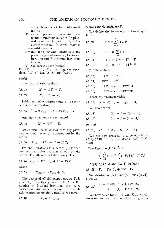
APPENDIX

Solution of the Model of the Soviet-Type Plan- ning Procedure with Internal Iterations

List of Symbols:

A = technology matrix-coefficients of input per unit output (matrix)

Qt = exogenously determined increments to aggregate outputs in year t (vector)

Dt= final demands in year t (vector) Yt= gross outputs in year t (vector) Xt= aggregate demands in year t (vec-

tor) Et= supply-demand imbalances in year

t (vector) Yt= preliminary aggregate output tar-

gets for year t (vector) Xt= initial tentative aggregate demands

for year t (vector) Yt(i)=tentative aggregate output targets

after i internal iterations (vector) Xt(i)= tentative aggregate demands after

i internal iterations (vector) Yt = official aggregate output targets for

year t (vector) Q= retrospective iteration parameter:

elements pertaining to commodities retrospectively iterated are set to 1,


other elements set to 0 (diagonal matrix)

r= central planning parameter: elements pertaining to centrally planned commodities set to 1, other elements set to 0 (diagonal matrix)

I= identity matrix N= number of ex ante iterations in the

planning procedure-i.e., 1 external iteration and N-1 internal iterations (scalar)

T= the current year (scalar) For J7n}, JIn], FI), IF[n], Qll), Q[], see equations (A.9)-(A.12), (A-18), and (A.19).

Model

Tautological relationships:

(A.1) Xt= AYt+Dt

(A. 2) Et = Yt -Xt

Initial tentative output targets are set (a retrospective iteration):

(A. 3) Yt = QXt_l + (I -Q) Yt- + Qt

Aggregate demands are estimated:

(A. 4) xt = A Yt + Dt

An external iteration (for centrally planned commodities only) is carried out by the center:

(A. 5) Yt (0 = r xt + (I-r Yt

Internal iterations (for centrally planned commodities only) are carried out by the center. The ith internal iteration yields:

(A. 6) Yt(j) = FXt(i_l) + (I - r) Yt

where

(A. 7) Xt(j) = A Yt(j) + Dt

The vector of official output targets Yt is given by Yt= Yt(AT1) where N-1 is the number of internal iterations that were carried out. And since it is assumed that official targets are precisely fulfilled, we have

(A. 8) Yt = Yt(X_1)

Solution for the modelfor ET

We define the following additional symbols:

n (A. 9) r(n) _-I (rA)i

i=o

n (A. 10) r [n] - E (Ar)i

i=O

(A. 11) r n-- rInj - r-n-I)r

(A. 12) r [n] -r[n - rrfn-11

It follows that:

(A. 13) AJr7{} = r(n1A

(A. 14) rr[n] = r(n)r

(A. 15) r n} = I + rr[n-1]A

(A. 1 6) r [n] = I + Arfn-l)r

These equivalences yield:

(A. 17) (I - A)rn} = r[] (I - A)

We also define:

(A. 18) Qtll I-Q(I-A)

(A. 19) Q[J] I-(I- A)Q

so that

(A. 20) (I - A)Qt} = Q1](I - A)

We can now proceed to solve equations (A.1)-(A.8) for ET. Equations (A.4)-(A.8) yield

Yt= Yt(N-1) = (FA)NYt +

( (FA)2-i (T`Dt+(I-r) Yt)

Applying (A.9) and (A.11) we have

(A. 21) Yt = F{N}Yt + ffN-1iFDt

Substitution of (A.1) and (A.3) into (A.21) gives us

Yt = I N}Q{(} Yt-1 + rFN}QDt_1

+ FfN}Qt + {FN-11}FDt

We now solve for Et-r[NIQ[[1IE.1, which turns out to be a function only of exogenous


variables and the parameters. By (A.1) and (A.2), we have

(A. 23) ''t = (I- A) Yt-Dt

Muiltiplying (A.23) lagged one period by .F[N]Q[1I, and subtracting the result from (A.23) yields:

Et - IFNQ[j3jEt-j = (I - A) Yt - Dt

- r[NIQ10](J - A) Yt-1 + r[NlQ[11Dt-,

and by using (A.17) and (A.20) we get

Et - PF(N12(1]Et1

(A. 24) (I - A)(Yt - TFN)Qti1 Yt-j)

- Dt + F[N]Q[1]Dt-1

But from (A.22) we have

Yt - r (NIQI)Yt-1

= F{N}IQDt- + FfNJQt + rT'N-1)rDt

and substituting this into (A.24) yields, after manipulations with (A.9)-(A.20), the following:

Et- r[N]2[1-]Et-

= r[N](Dt- - Dj) + F[N](I - A)Qt

Or, defining ADt=Dt-Dt-1 , we have

Et - rF[N)Q[jjEt- (A. 2 5)

= r [NI(Qt - (AQt + ADt))

Solving (A.25) as a difference equation in t, we get

T

ET = E (r[N]U[l])Tp [AN] (A. 26) t=1

(Qt - (A Qt + ADt))

+ (Fp[N]Q[f])TEo

Equation (A.26) is a general solution for ET when the planning procedure includes one external iteration and N- 1 internal iterations. When the planning procedure includes no internal iterations (N = 1), and given that Eo=O, the solution reduces to equation (14).

REFERENCES

A. Dorovskikh, "Nekotorie voprosi teori i praktiki mezhotraslevogo balansa," (Some Questions on the Theory and Practice of the Interbranch Balance), Planovoe Khozi- aistvo, Dec. 1967, 44, 35-44.

M. R. Eidel'man, Mezliotraslevoi Balans Ob- shchestvennogo Produkta, (The Interbranch Balance of the Social Product), Moscow 1966.

M. Ellman, "The Consistency of Soviet Plans," Scot. J. Polit. Econ., Feb. 1969, 16, 50-74.

I. A. Evenko, Planning in the USSR, Moscow 1962.

H. S. Levine, "The Centralized Planning of Supply in Soviet Industry," in Joint Eco- nomic Committee, U.S. Congress, Compari- sons of the United States and Soviet Econo- mies, Washington 1959, 151-76.

"Pressure and Planning in the Soviet Economy," in H. Rosovsky ed., Industriali- zation in Two Systems: Essays in ,Honor of Alexander Gerschenkron, New York 1966, 266-85. -- , "A Study in Economic Planning,"

unpublished doctoral dissertation, Harvard Univ. 1961.

M. Manove, "A Model of Administrative Plan- ning and Plan Execution in Soviet-Type Economies," unpublished doctoral dissertation, M.I.T. 1970.

J. M. Montias, Central Planning in Poland, New Haven 1962.

, "On the Consistency and Efficiency of Central Plans," Rev. Econ. Stud., Oct. 1962, 29, 280-93.

"Planning with Material Balances in Soviet-type Economies," Amer. Econ. Rev., Dec. 1959, 49, 963-85.

G. Sorokin, Planning in the USSR, Moscow 1967.

R. Stone, "Consistent Projection in Multi- Sectoral Models," in E. Mailinvaud and M. Bacharach, eds., Activity Analysis in the Theory of Growth and Planning, New York 1967, 232-34.

V. G. Treml, "The 1959 Soviet Input-Output Table (as Reconstructed) ," in Joint Eco-


nomic Committee, U.S. Congress, New Di- rections in the Soviet Economy, Part II-A, Washington 1966, 259-70.

"New Soviet Interindustry Data," in Joint Economic Committee, U.S. Congress,

Soviet Economic Performance: 1966-1967, Washington 1968, 145-58.

P. Weitzman, "Planning Consumption in the USSR," unpublished doctoral dissertation, Univ. Mich. 1969.

Documents

A Model of Soviet-Type Economic Planning