Embed Size (px)
Citation preview
1
A Model of Nonlinear Urbanization and
Information Flows Across India
Chris Shughrue
Karen C. Seto, Advisor Hixon Center for Urban Ecology
March 4, 2013
2
Abstract
Urbanization in the 21st century is increasingly shaped by distal flows of
people, capital, and information across the landscape. In India, these flows are predicated
on expectations informed by the propagation of information across social networks.
Networks across rural-urban boundaries and between urban centers are a principle
mechanism underlying migration and investment patterns. These patterns shape and are
shaped by the growth of city-regions. Our driving research question is: How does the
strength of signal propagation across social networks underlying spatial flows affect
emergent patterns of urban land-use change? To examine this relationship, we developed
an agent-based model of regional-scale urbanization for the extent of India on a spatially
explicit grid derived from satellite data wherein we represent the dynamics of decisions
made by: land developers, families, state governments, corporations, and property
management companies. Decisions made by family agents are based on information
propagated across an adaptive social network. We varied the probability of data
transmission across the network to simulate the effects of strong and weak social
networks on spatial patterns of urbanization.
Introduction
Most of the projected urbanization in India is expected to occur over the next
two decades (United Nations, 2012). This growth will account for roughly 16% of the
global increase in urban population. Urban expansion is increasingly being shaped by
distal flows of people, materials, and information across the landscape rather than local
processes (Seto, 2012). The dynamics that underlie these flows in India have been rapidly
changing since liberalization in 1991.
3
Since liberalization, India has been undergoing a social and economic
transition. Foreign direct investment has increased by several orders of magnitude over
this period (Singh, 2005). With the influx of a multitude of new tertiary sector labor
opportunities, the value of education has increased. The number of people investing in
higher education has tripled on the interval between 1991 and 2005 (Agarwal, 2006).
Many of these new labor and educational opportunities are located in major cities,
drawing people from across the country (Seto, 2011). The simultaneous increase in
skilled labor and desirable labor opportunities driven by multinational investment has
been accompanied by an increase in the rate of migration from rural to urban and
between urban areas.
The process of information and human capital moving across the landscape is
facilitated by and results in the formation of social networks (Kossinets, 2006). In India,
social networks are the principle mechanism by which information about housing and
labor opportunities is propagated (Banerjee, 1981; Banerjee, 1984; Kerr, 2011). The
behavior of complex ad hoc networks is related to connectivity and conductivity
(Newman, 2003). As a result, the pathways by which information is propagated across
the network affects decisions made by families, and is affected by consequent decisions
to relocate, for example. The adaptation of networks of flows, including information and
human, is a mechanism by which cities are capable of self-organizing on a regional scale
(Batty, 2008). The formation and adaptation of these networks is a dynamic process that
affects and is affected by the development of the urban environment. It is difficult to
predict how properties of the network will affect the emergence of regional-scale
urbanization because these networks are embedded in a complex system comprised of
4
economic, physical, and social subsystem. Our objective is to understand how the
strength of signal propagation across the social networks underlying human and capital
flows will affect emergent urbanization patterns.
Equilibrium models of urbanization are largely incapable of dealing with
nonlinearities captured within long-time-scale system boundaries (Feigenbaum, 2003).
This set of methodologies is incompatible with representing regional dynamics of
urbanization – on this scale cities are open systems that exchange people, materials, and
information nonlinearly (Allen, 1997). Dynamical models are capable of representing the
underlying processes of urbanization with mechanisms for co-adaptation and evolution
(Werner, 2007). Allen (1997) and Batty (2001), for example, have used dynamical
models for land cover change but these models did not attempt to represent actual
decision making processes or aspatial network formation. These models are useful in
exploring the theoretical implications of urban networks, but offer no insight into the
workings of actual cities.
Our approach is to approximate human decision-making (following: McNamara
and Werner, 2008a,b); in a dynamical model to explore system stability and adaptability
(Alberti, 2000). The output from this spatially explicit agent-based model will be used to
assess how properties of social networks affect urbanization through adaptive
socioeconomic systems. We will examine the effects of properties of network formation
on patterns of urbanization.
Model
The simulation is a spatially explicit model that represents the decision-making
process of land developers, property managers, families, state governments, and
5
multinational corporations in India. These processes are categorized into modules by
agent type to facilitate description. Each agent makes decisions, described in the sections
below, to approximate decisions made by actors in the system on annual to decadal time
scales.
Grid
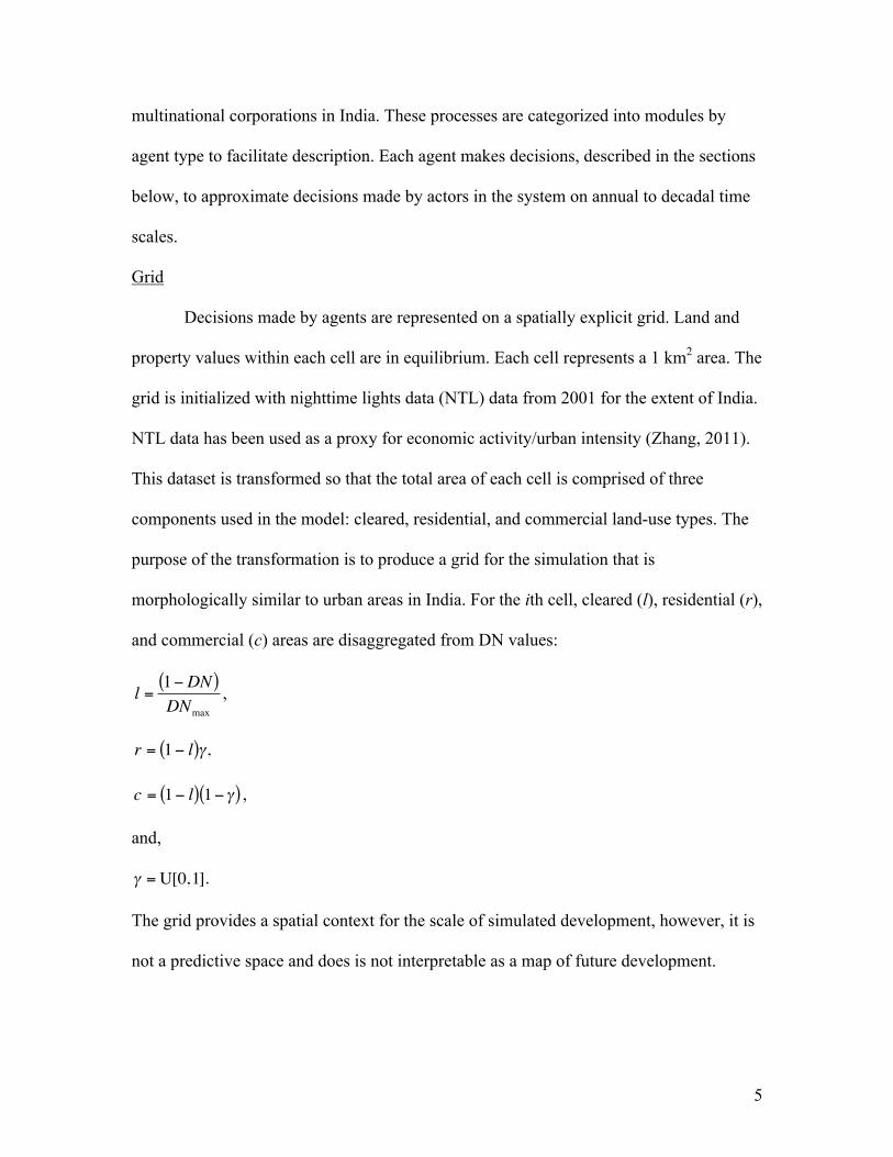
Decisions made by agents are represented on a spatially explicit grid. Land and
property values within each cell are in equilibrium. Each cell represents a 1 km2 area. The
grid is initialized with nighttime lights data (NTL) data from 2001 for the extent of India.
NTL data has been used as a proxy for economic activity/urban intensity (Zhang, 2011).
This dataset is transformed so that the total area of each cell is comprised of three
components used in the model: cleared, residential, and commercial land-use types. The
purpose of the transformation is to produce a grid for the simulation that is
morphologically similar to urban areas in India. For the ith cell, cleared (l), residential (r),
and commercial (c) areas are disaggregated from DN values:
€
l =1−DN( )DNmax
,
€
r = 1− l( )γ,
€
c = 1− l( ) 1−γ( ) ,
and,
€
γ =U[0,1].
The grid provides a spatial context for the scale of simulated development, however, it is
not a predictive space and does is not interpretable as a map of future development.
6
Figure 1 Initial grid simulated from NTL data (2001). Each cell is comprised of open space (red), commercial (blue) and residential (green) components.
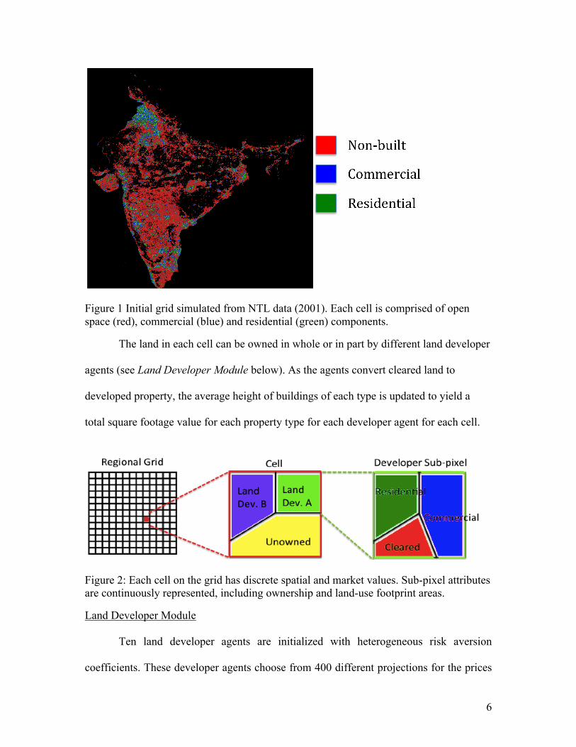
The land in each cell can be owned in whole or in part by different land developer
agents (see Land Developer Module below). As the agents convert cleared land to
developed property, the average height of buildings of each type is updated to yield a
total square footage value for each property type for each developer agent for each cell.
Figure 2: Each cell on the grid has discrete spatial and market values. Sub-pixel attributes are continuously represented, including ownership and land-use footprint areas.
Land Developer Module
Ten land developer agents are initialized with heterogeneous risk aversion
coefficients. These developer agents choose from 400 different projections for the prices
7
of land and commercial and residential property in each cell. Land developer agents
employ the model with the lowest variance plus small nonsystematic noise (Werner,
2008). Each land developer agent evaluates the expected profit and risk of purchasing
land and constructing buildings on each parcel of land. The demand for the number of
areal units of a building for the ith agent in the jth tract is n (Gennotte and Leland, 1990;
Feigenbaum, 2003):
€
n =pij h j
* − 1+ r( )C(h j* )l jh j
*
ω iσ ij2 ,
where
€
p is the projected price per square foot completed floor space in the jth cell, r is
the safe rate of return, C is the cost function for the mean price per square foot of
construction of a building with optimal height,
€
h* . The cost function, C yields the
average price of floor space construction as a power function of height, h, (Mann, 1992):
€
C = p 1+α( )h . (1)
The price of land is l,
€
ω is the risk aversion coefficient for the ith land developer
agent, and
€
σ2 is the estimated variance of the price projection. The optimal building
height, h*, is the numerical solution of:
€
αh3 + h2 − lp0 ln 1+α( )
= 0 .
This function is the solution to the minimization of the average cost of construction per
square foot including land price, l, which is a modification of equation 1 above:
€ €
C = p 1+α( )h +lh
.
Agents appraise available property and invest in a portfolio of projects with the greatest
cumulative demand that does not exceed a fixed annual budget.
8
Developer agents acquire land from the state government through a competitive
bidding process. For the jth parcel, the ith interested land developer agent submits a
proposal for the quantity of land and a price, Gij:
€
Gij = α i p j
where pj is the current value of land at the jth parcel and
€
α i is the bidding ratio employed
by the ith agent. The state government distributes the full amount of land requested to
bidders in order of highest bid until all available land in j is distributed. The optimal
bidding amount is an infinitesimal increment greater than the second place bid for all
cells. Agents track bidding errors with respect to the optimal bid,
€
E . Agents adjust
€
α
adaptively to minimize bidding errors, both over and underbidding (Dasgupta and Das,
2000):
€
α t+1 = α t +δ t sign α t −α t−1( )sign Et−1 − Et( ),
where,
€
δ t = δ t−1εsign Et−1 −Et( ),
and
€
ε is a small constant parameter.
Property Manager Module
Ten property manager agents invest in residential and commercial space on the
grid and rent this stock to firm and family agents to maximize profit from both property
speculation and rental revenue. Property manager agents project property values and
rental rates across space using the same projection models as the land developer agents.
The demand for the amount of property space by the ith property manager agent in the jth
cell is n (Gennotte and Leland, 1990; Feigenbaum, 2003):
9
€
n =Rij + pij − p j 1+ r( )
ω iσ ij2 ,
where
€
R and
€
p are the projected rental rates and property values for the next time
step, respectively, and p is the current property value. Agents make offers on the optimal
portfolio of properties within a fixed budget. When the demand for property exceeds
supply, the fraction of available land awarded to the ith property manager agent, fi, is:
€
fi =nini
i=1∑
.
Family Module
In the model, family agents make decisions about where to live and work in order
to maximize income. All information used to make these decisions is propagated across a
spatially explicit social network. Banerjee (1984) and Mitra (2004) describe
informational remittances by immigrants to their hometowns as driving migration
patterns. Propagation of information in the model represents both spatially local diffusion
(through random interactions) and information shared about the current location of a
family with the “home” cell where the family formed. Estimates for values on the grid are
produced with an inverse distance weighted average (IDW) using available observations:
€
u(x) =χwi(x)u(xi)
w j (x)j=0
N∑i=0
N
∑ ,
where,
€
wi(x) = d(x,xi)−1,
and
€
u(xi) is the value of the ith observation, d is the distance between the ith cell and an
arbitrary cell, x. The spatial interpolation available to family agents in the ith cell
10
incorporates observations at cells where family agents that originated in the ith cell are
currently located. Interpolations for the ith cell are averaged (IDW) with local cells to
account for information sharing. Observations with a weight less than 0.1 are ignored for
computational efficiency.
IDW averages are propagated between cells where there is at least one family that
originated and currently resides in either cell to represent informational remittances by
families that move. These distal IDW averages are averaged with local IDW averages to
incorporate both types of data. Averages used by agents in subsequent modules are
generally limited to information that has been propagated across the network.
A dissipation parameter,
€
χ, is varied between 0 and 1 and represents that
probability that information is propagated across the network at the ith cell. When
€
χ is 0,
members of the same social network have perfect knowledge of all observations in the
network. As
€
χ approaches 1, the probability of each observation being diffused and
propagated approaches 0. The variation of this parameter will be used to examine how
the strength of social network signal propagation affects urbanization.
Migration is driven by a combination of push and pull factors (Kainth, 2010). A
primary push factor is lack of economic opportunity. Family agents compare current
aggregate income against average opportunities as informed by their respective social
network. The income differential between current and expected opportunities, K,
represents an estimate of push factors:
€
K = H + e weRe∑ + n wnRn∑( ) − W + H( ) ,
where W is the current total wages earned by the family, H is the current rent paid for
housing, e is the number of educated family members, and n is the number of non-
11
educated family members.
€
w is the mean wage across the social network,
€
R is the
mean employment rate across the social network, and the subscripts e and n denote
educated and non-educated, respectively.
€
H is the mean rent across the social network.
Family agents with positive K become prospective migrants.
Prospective migrant agents estimate the value of pull factors, B, for each cell on
the grid:
€
B = e weRe + n wnRn − H + m( ) ,
where
€
m is the IDW average of transportation cost, which is a linear function of
distance between the ith cell and cells with labor opportunities. H is the rental cost in the
ith cell and
€
wR is the IDW average of wages and employment rates in cells with
employment opportunities neighboring the ith housing cell. Prospective migrants choose
to move to the cell where B is maximized. In cases where the demand for rental space in
a cell exceeds the available space, units are randomly distributed to applicants, and
unsuccessful applicants do not move.
Casual labor and retail sectors are significant segments of the Indian economy,
and urban space consumers. In this version of the model, these segments are reduced to a
linear scale with population density. For each person agent in a given cell, a demand for
commercial space, dR, is:
€
dR = αRK,
where
€
αR is a conversion factor that relates total population in each cell, K, to the retail
economies associated with that population. This demand draws on available commercial
space and may affect the price of commercial space using the same mechanism for
renting as for families, however, the source of money for rent is external.
12
Education Module
Family agents are each comprised of subagent workers, which are defined by an
age, skill level, and income. Uneducated people subagents currently located in the ith
cell calculate the expected value of investing in education using information propagated
across their social network:
€
B = L weRe − w[ ] − T ,
where the subscript
€
we is the mean wage for educated labor,
€
Re is the employment
rate for educated. w is the current wage for the worked (unemployed workers use mean
wage and employment rate estimates across the social network). L is the difference
between current age and maximum working age, and
€
T is the mean tuition across the
network. When B is positive and
€
T < family agent capital, people subagents become
prospective students.
Prospective students choose an optimal location for education by maximizing
total income, I:
€
I = L wR − T +H +m( ) ,
where
€
wR is the product of the IDW averages of post-graduate wage and employment
rate for universities surrounding the ith cell. T, H, and m are the IDW averages of tuition,
housing rent for an individual, and transportation costs in the ith cell. H is 0 for the cell
where the corresponding family agent currently lives. m is a linear function of distance
between the housing cell and the university cell. When the optimal cell is not coincident
with the family agent, the prospective subagent nucleates to form a separate family agent
and moves for school.
IT and Manufacturing Firms
13
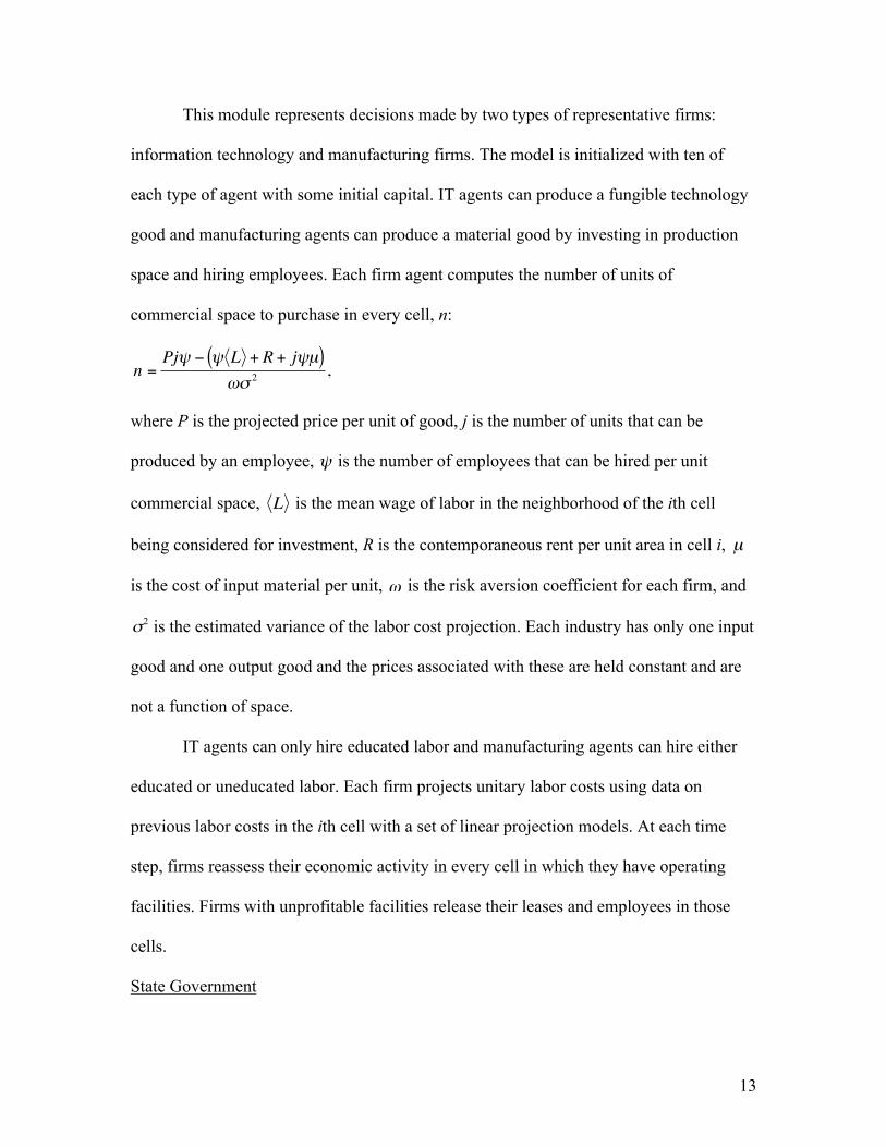
This module represents decisions made by two types of representative firms:
information technology and manufacturing firms. The model is initialized with ten of
each type of agent with some initial capital. IT agents can produce a fungible technology
good and manufacturing agents can produce a material good by investing in production
space and hiring employees. Each firm agent computes the number of units of
commercial space to purchase in every cell, n:
€
n =Pjψ − ψ L + R + jψµ( )
ωσ 2 ,
where P is the projected price per unit of good, j is the number of units that can be
produced by an employee,
€
ψ is the number of employees that can be hired per unit
commercial space,
€
L is the mean wage of labor in the neighborhood of the ith cell
being considered for investment, R is the contemporaneous rent per unit area in cell i,
€
µ
is the cost of input material per unit,
€
ω is the risk aversion coefficient for each firm, and
€
σ2 is the estimated variance of the labor cost projection. Each industry has only one input
good and one output good and the prices associated with these are held constant and are
not a function of space.
IT agents can only hire educated labor and manufacturing agents can hire either
educated or uneducated labor. Each firm projects unitary labor costs using data on
previous labor costs in the ith cell with a set of linear projection models. At each time
step, firms reassess their economic activity in every cell in which they have operating
facilities. Firms with unprofitable facilities release their leases and employees in those
cells.
State Government
14
State agents make decisions about which cells to designate as development areas
and investment in colleges. In this version, each state opens a small number of cells for
development at the end of each time step. Each new cell must be contiguous to existing
development cells. In future, this mechanism will incorporate a cost-benefit analysis to
weigh the expected income from new development against costs associated with
agricultural land and tax revenue loss.
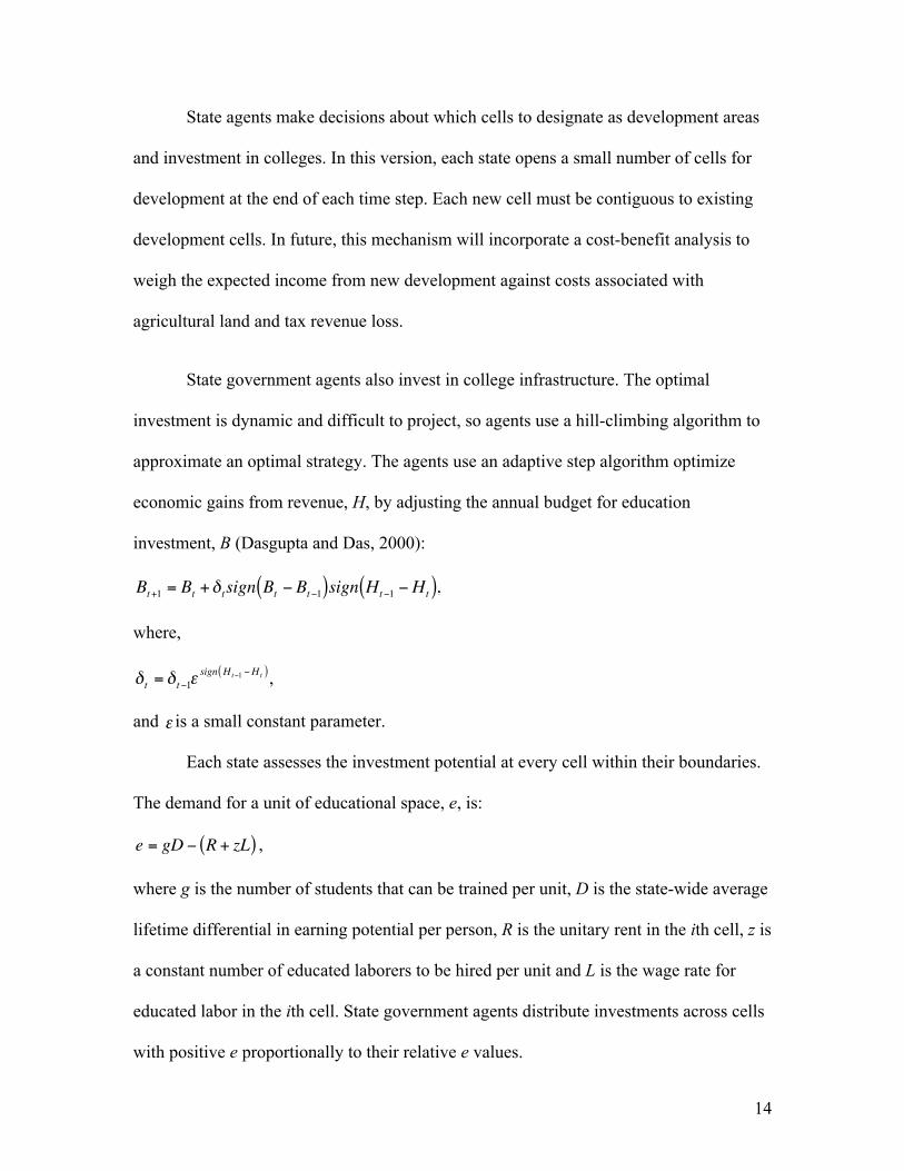
State government agents also invest in college infrastructure. The optimal
investment is dynamic and difficult to project, so agents use a hill-climbing algorithm to
approximate an optimal strategy. The agents use an adaptive step algorithm optimize
economic gains from revenue, H, by adjusting the annual budget for education
investment, B (Dasgupta and Das, 2000):
€
Bt+1 = Bt +δ t sign Bt − Bt−1( )sign Ht−1 −Ht( ),
where,
€
δ t = δ t−1εsign Ht−1 −Ht( ),
and
€
ε is a small constant parameter.
Each state assesses the investment potential at every cell within their boundaries.
The demand for a unit of educational space, e, is:
€
e = gD − R + zL( ) ,
where g is the number of students that can be trained per unit, D is the state-wide average
lifetime differential in earning potential per person, R is the unitary rent in the ith cell, z is
a constant number of educated laborers to be hired per unit and L is the wage rate for
educated labor in the ith cell. State government agents distribute investments across cells
with positive e proportionally to their relative e values.
15
Land and Property Markets
Land and property prices are endogenously determined in the model. Prices adjust
dynamically as a function of demand, D, and supply, S, (Nicholson, 1995):
€
dPdt
= α p D − S( ) ,
where
€
α p is a constant of proportionality.
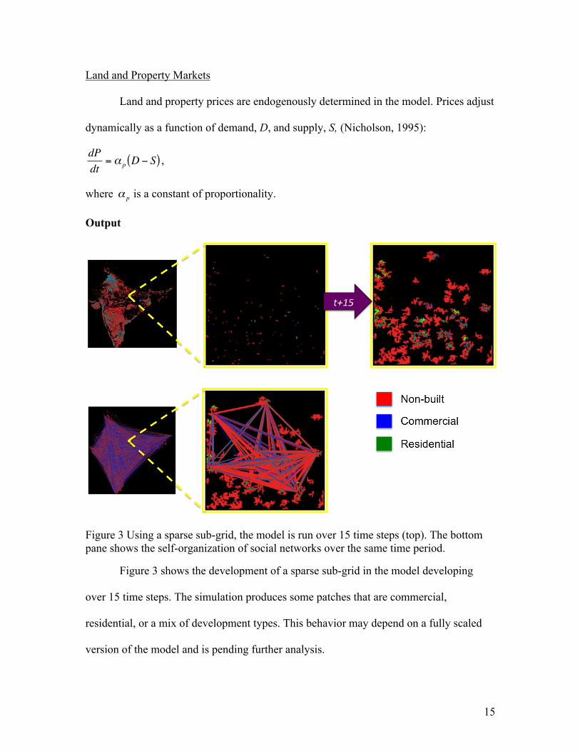
Output
Figure 3 Using a sparse sub-grid, the model is run over 15 time steps (top). The bottom pane shows the self-organization of social networks over the same time period.
Figure 3 shows the development of a sparse sub-grid in the model developing
over 15 time steps. The simulation produces some patches that are commercial,
residential, or a mix of development types. This behavior may depend on a fully scaled
version of the model and is pending further analysis.
16
Social networks are initialized with random nodes. The lower pane shows the
self-organization of networks into coherent connections between clusters of urban areas
on the grid by time step 15. Some parcels on the grid are not connected to the social
network because families have not yet moved to these cells, which were developed
rapidly in previous time steps.
Next Steps
The model encounters several computational bottlenecks associated with the
social network diffusion algorithms that scale with the density of urban cells on the grid.
These computations will be broken into several pieces for parallelization on the Yale
High Performance Cluster. After this, the model will be capable of running on the entire
extent of India for densities where the number of urban cells approaches the total number
of cells.
The fully scaled version of the model will be run with variations of the parameter
controlling the dissipation of information across the social networks,
€
χ. This parameter
represents the connectivity of social networks, which is related to changes in social
behavior. The variation in this parameter will be compared to time series of urbanization
on the grid in terms of: land use change, land use type, fragmentation, and cell cluster
size and contiguity. The model will be run over multiple random number generators to
estimate the effect of stochasticity on the model results, and parameters with estimated
values will be assessed with a sensitivity analysis.
17
References
Agarwal, P. (2006). Higher education in India: The need for change, (180).
Alberti, M., & Waddell, P. (2000). An integrated urban development and ecological
simulation model. Landscape Ecology, 1, 215–227.
Allen, Peter Murray M. Cities and Regions as Self-Organizing Systems : Models of
Complexity. Gordon & Breach Publishing Group, (1997).
Batty, M. (2008). The size, scale, and shape of cities. Science (New York, N.Y.),
319(5864), 769–71.
Batty, M. (2001). Polynucleated Urban Landscapes. Urban Studies, 38(4), 635–655.
Banerjee, B. (1984). Information Flow, Expectations and Job Search: Rural-to-Urban
Migration Process in India. International Monetary Fund, 1, 239–257.
Dasgupta, P. (2000). Dynamic pricing with limited competitor information in a multi-
agent economy. Cooperative Information Systems, 299–310.
Feigenbaum, J. (2003). Financial physics. Reports on Progress in Physics, 66(10), 1611–
1649.
Gennotte, G., & Leland, H. (1990). Market liquidity, hedging, and crashes. The American
Economic Review, 80(5).
Kossinets, G., & Watts, D. J. (2006). Empirical analysis of an evolving social network.
Science (New York, N.Y.), 311(5757), 88–90.
Mann, T. (1992). Building Economics for Architects, Van Nostrand Reinhold, New York,
NY.
18
McNamara, D. E., & Werner, B. T. (2008a). Coupled barrier island–resort model: 1.
Emergent instabilities induced by strong human-landscape interactions. Journal of
Geophysical Research, 113(F1), 1–10.
McNamara, D. E., & Werner, B. T. (2008). Coupled barrier island–resort model: 2. Tests
and predictions along Ocean City and Assateague Island National Seashore,
Maryland. Journal of Geophysical Research, 113(F1), 1–9.
Mitra, A. (2004). Informal Sector, Networks and Intra-City Variations in Activities:
Findings From Delhi Slums. Review of Urban and Regional Development Studies,
16(2), 154–169.
Nicholson, W. (1985), Microeconomic Theory: Basic Principles and Extensions, Dryden
Press, Chicago, Ill.
Parker, D. C., & Meretsky, V. (2004). Measuring pattern outcomes in an agent-based
model of edge-effect externalities using spatial metrics. Agriculture, Ecosystems &
Environment, 101(2-3), 233–250.
Seto, K. C. (2011). Exploring the dynamics of migration to mega-delta cities in Asia and
Africa: Contemporary drivers and future scenarios. Global Environmental Change,
2100.
Seto, K. C., Reenberg, A., Boone, C. G., Fragkias, M., Haase, D., Langanke, T.,
Marcotullio, P., et al. (2012). Urban land teleconnections and sustainability, 1–6.
Singh, G. S. (2010). Push and Pull Factors of Migration: A Case Study of Brick Kiln
Migrant Workers in Punjab.
Singh, K. (2005). Foreign direct investment in India: A critical Analysis of FDI from
1991-2005. Analysis.
19
United Nations. (2012). World Urbanization Prospects The 2011 Revision. Population.
Werner, B. T., & McNamara, D. E. (2007). Dynamics of coupled human-landscape
systems. Geomorphology, 91(3-4), 393–407.
Zhang, Q., & Seto, K. C. (2011). Mapping urbanization dynamics at regional and global
scales using multi-temporal DMSP/OLS nighttime light data. Remote Sensing of
Environment, 115(9), 2320–2329. doi:10.1016/j.rse.2011.04.032