Embed Size (px)
Citation preview

A Model of Mortgage Default
John Y. Campbell1
João F. Cocco2
This version: February 2014
First draft: November 2010
JEL classi�cation: G21, E21.
Keywords: Household �nance, loan to value ratio, loan to income ratio, mortgage a¤ordability,
negative home equity, mortgage premia.1Department of Economics, Harvard University, Littauer Center, Cambridge, MA 02138, US and NBER.
Email [email protected] of Finance, London Business School, Regent�s Park, London NW1 4SA, UK, CEPR, CFS and
Netspar. Email [email protected]. We would like to thank seminar participants at the AEA 2012 meetings,
Bank of England, Berkeley, Bocconi, Essec, the 2012 SIFR Conference on Real Estate and Mortgage Finance,
the 2011 Spring HULM Conference, Illinois, London Business School, Mannheim, the Federal Reserve Bank of
Minneapolis, Norges Bank, and the Rodney L. White Center for Financial Research at the Wharton School,
and Stefano Corradin, Andra Ghent, Francisco Gomes, John Heaton, Jonathan Heathcote, Pat Kehoe, Ellen
McGrattan, Steve LeRoy, Jim Poterba, Nikolai Roussanov, Sam Schulhofer-Wohl, Roine Vestman, and Paul
Willen for helpful comments on an earlier version of this paper. We are particularly grateful to three anonymous
referees and to Ken Singleton (editor) for comments that have signifcantly improved the paper.

Abstract
This paper solves a dynamic model of households�mortgage decisions incorporating labor in-
come, house price, in�ation, and interest rate risk. It uses a zero-pro�t condition for mortgage
lenders to solve for equilibrium mortgage rates given borrower characteristics and optimal de-
cisions. The model quanti�es the e¤ects of adjustable vs. �xed mortgage rates, loan-to-value
ratios, and mortgage a¤ordability measures on mortgage premia and default. Heterogeneity in
borrowers�labor income risk is important for explaining the higher default rates on adjustable-
rate mortgages during the recent US housing downturn, and the variation in mortgage premia
with the level of interest rates.

1 Introduction
The early years of the 21st Century were characterized by unprecedented instability in house
prices and mortgage market conditions, both in the US and globally. After the housing credit
boom in the mid-2000s, the housing downturn of the late 2000s saw dramatic increases in
mortgage defaults. Losses to mortgage lenders stressed the �nancial system and contributed to
the larger economic downturn. These events have underscored the importance of understanding
household incentives to default on mortgages, and the way in which these incentives vary across
di¤erent types of mortgage contracts.
This paper studies the mortgage default decision using a theoretical model of a rational
utility-maximizing household. We solve a dynamic model of a household who �nances the
purchase of a house with a mortgage, and who must in each period decide how much to consume
and whether to exercise options to default, prepay or re�nance the loan. Several sources of risk
a¤ect household decisions and the value of the options on the mortgage, including house prices,
labor income, in�ation, and real interest rates. We use multiple data sources to parameterize
these risks.
Importantly, we study household decisions for endogenously determined mortgage rates.
We model the cash �ows of mortgage providers, including a loss on the value of the house in
the event the household defaults. We then use risk-adjusted discount rates and a zero-pro�t
condition to determine the mortgage premia that in equilibrium should apply to each contract.
Since household mortgage decisions depend on interest rates and mortgage premia, and these
decisions a¤ect the pro�ts of banks, we must solve several iterations of our model for each
mortgage contract to �nd a �xed point. Thus our model is not only a model of mortgage
default, but also a micro-founded model of the determination of mortgage premia.
The literature on mortgage default has emphasized the role of house prices and home equity
accumulation for the default decision. Deng, Quigley, and Van Order (2000) estimate a model,
based on option theory, in which a household�s option to default is exercised if it is in the money
by some speci�c amount. Borrowers do not default as soon as home equity becomes negative;
they prefer to wait since default is irreversible and house prices may increase. Earlier empirical
papers by Vandell (1978) and Campbell and Dietrich (1983) also emphasized the importance
of home equity for the default decision.

In our model also, mortgage default is triggered by negative home equity which tends to
occur for a particular combination of the several shocks that the household faces: house price
declines in a low in�ation environment with large nominal mortgage balances outstanding. As
in the previous literature, households do not default as soon as home equity becomes negative.
A novel prediction of our model is that the level of negative home equity that triggers default
depends on the extent to which households are borrowing constrained. As house prices decline,
households with tightly binding borrowing constraints will default sooner than unconstrained
households, because they value the immediate budget relief from default more highly relative
to the longer-term costs. The degree to which borrowing constraints bind depends on the
realizations of income shocks, the endogenously chosen level of savings, the level of interest rates,
and the terms of the mortgage contract. For example, adjustable-rate mortgages (ARMs) tend
to default when interest rates increase, because high interest rates increase required mortgage
payments on ARMs, tightening borrowing constraints and triggering defaults.
We use our model to illustrate these triggers for mortgage default and to explore several
interesting questions about the e¤ects of the mortgage system on defaults and mortgage premia.
First, we use our model to understand how the adjustability of mortgage rates a¤ects de-
fault behavior, comparing default rates for adjustable-rate mortgages (ARMs) and �xed-rate
mortgages (FRMs). Unsurprisingly, both ARMs and FRMs experience high default rates when
there are large declines in house prices. However, for aggregate states with moderate declines
in house prices, ARM defaults tend to occur when interest rates are high� because high rates
increase the required payments on ARMs� whereas the reverse is true for FRMs.
Second, we determine mortgage premia in the model and compare the results to the data.
For most parameterizations and household characteristics the model predicts that mortgage
premia should increase with the level of interest rates. In US data this appears to be the
case for FRMs, but not for ARMs. The model is able to generate ARM premia that decrease
with interest rates when we assume that ARM borrowers have labor income that is not only
riskier on average, but also correlated with the level of interest rates. Such a correlation arises
naturally if interest rates tend to be lower in recessions. We use our model to perform welfare
calculations and show that households with this type of income risk bene�t more from ARMs
relative to FRMs, supporting the hypothesis that such households disproportionately borrow
at adjustable rates.
2

Even though our model can generate the qualitative patterns of mortgage premia observed
in the data, it is harder to match those patterns quantitatively. Our model does not easily
explain the large ARM premia observed in US data when interest rates are low. Furthermore,
our model generally predicts a larger positive e¤ect of interest rates on FRM mortgage premia
than the one observed in US data. Our model can deliver FRM mortgage premia that better
match the data if there is re�nancing inertia (Miles 2004, Campbell 2006), so that households
do not re�nance their FRMs as soon as it is optimal to do so.
Third, we ask how ratios at mortgage origination such as loan-to-value (LTV), loan-to-
income (LTI), and mortgage-payments-to-income (MTI) a¤ect default probabilities. The LTV
ratio measures the household�s initial equity stake, while LTI and MTI are measures of initial
mortgage a¤ordability. A clear understanding of the relation between these ratios and mortgage
defaults is particularly important in light of the recent US experience. Figure 1 plots aggregate
ratios for newly originated US mortgages over the last couple of decades, using data from the
monthly interest rate survey of mortgage lenders conducted by the Federal Housing Finance
Agency.3 This �gure shows that there was an increase in the average LTV in the years before
the crisis, but to a level that does not seem high by historical standards. A caveat is that
the survey omits information on second mortgages, which became far more common during
the 2000s.4 Even looking only at �rst mortgages, however, there is a striking increase in the
average LTI ratio, from an average of 3.3 during the 1980�s and 1990�s to a value as high as
4.5 in the mid 2000s. This pattern in the LTI ratio is not con�ned to the US; in the United
Kingdom the average LTI ratio increased from roughly two in the 1970�s and 1980�s to above
3.5 in the years leading to the credit crunch (Financial Services Authority, 2009). Interestingly,
as can be seen from Figure 1, the low interest-rate environment in the 2000s prevented the
increase in LTI from driving up MTI to any great extent.
Our model allows us to understand the channels through which LTV and initial mortgage
a¤ordability ratios a¤ect mortgage default. A higher LTV ratio (equivalently, smaller down-
payment) increases the probability of negative home equity and mortgage default, an e¤ect that
3The LTV series is taken directly from the survey, and the LTI series is calculated as the ratio of average
loan amount obtained from the same survey to the median US household income obtained from census data.
The survey is available at www.fhfa.gov.4In addition the �gure shows the average LTV, not the right tail of the distribution of LTVs which may be
relevant for mortgage default.
3

has been documented empirically by Schwartz and Torous (2003) and more recently by Mayer,
Pence, and Sherlund (2009). The unconditional default probabilities predicted by our model
become particularly large for LTV ratios in excess of ninety percent.
The LTI ratio a¤ects default probabilities through a di¤erent channel. A higher initial
LTI ratio does not increase the probability of negative equity; however, it reduces mortgage
a¤ordability making borrowing constraints more likely to bind. The level of negative home
equity that triggers default becomes less negative, and default probabilities accordingly increase.
Our model implies that mortgage providers and regulators should think about combinations of
LTV and LTI and should not try to control these parameters in isolation.5
Fourth, we model heterogeneity in labor income growth, labor income risk, and other house-
hold characteristics such as intertemporal preferences and inherent reluctance to default. For
instance, we consider two households who have the same current income, but who di¤er in terms
of the expected growth rate of their labor income. The higher the growth rate, the smaller are
the incentives to save, which increases default probabilities. However, we �nd that this e¤ect
is slightly weaker than the direct e¤ect of higher future income on mortgage a¤ordability, as
measured for example by the MTI ratio later in the life of the loan. Therefore the mortgage
default rate and the equilibrium mortgage premium decrease with the expected growth rate of
labor income.
Finally, we use our model to simulate developments during a downturn like the one experi-
enced by the US in the late 2000s. One motivation for this exercise is that during the downturn
US default rates were considerably higher for ARMs than for FRMs, even though interest rates
were declining, which contradicts our model�s prediction that ARMs default primarily when
interest rates increase. To try to understand this fact we simulate our model for a path for
aggregate variables that matches the recent US experience of declining house prices and low
interest rates. We show that one explanation for the higher default rates of ARMs is that
ARMs are particularly attractive to households who face higher labor income risk, particularly
5Regulators in many countries, including Austria, Poland, China and Hong Kong, ban high LTV ratios in
an e¤ort to control the incidence of mortgage default. Some countries, such as the Netherlands, China, and
Hong Kong, have also imposed thresholds on the mortgage a¤ordability ratios LTI and MTI, either in the form
of guidelines or strict limits. For instance, in Hong Kong, in 1999, the maximum LTV of 70% was increased to
90% provided that borrowers satis�ed a set of eligibility criteria based on a maximum debt-to-income ratio, a
maximum loan amount, and a maximum loan maturity at mortgage origination.
4

if their labor income is correlated with interest rates. In addition we model ARMs with a teaser
rate to capture the fact that interest-only and other alternative mortgage products have had
higher delinquency and default rates than traditional principal-repayment mortgages (Mayer,
Pence, and Sherlund, 2009).
Several recent empirical papers study mortgage default. Foote, Gerardi, and Willen (2008)
examine homeowners in Massachusetts who had negative home equity during the early 1990s
and �nd that fewer than 10% of these owners eventually lost their home to foreclosure, so that
not all households with negative home equity default. Bajari, Chu, and Park (2009) study
empirically the relative importance of the various drivers behind subprime borrowers�decision
to default. They emphasize the role of the nationwide decrease in home prices as the main driver
of default, but also �nd that the increase in borrowers with high payment to income ratios has
contributed to increased default rates in the subprime market. Mian and Su�(2009) emphasize
the importance of an increase in mortgage supply in the mid-2000s, driven by securitization
that created moral hazard among mortgage originators.
The contribution of our paper is to propose a dynamic and uni�ed microeconomic model of
rational consumption and mortgage default in the presence of house price, labor income, and
interest rate risk. Our goal is not to try to derive the optimal mortgage contract (as in Pisko-
rski and Tchistyi, 2010, 2011), but instead to study the determinants of the default decision
within an empirically parameterized model, and to compare outcomes across di¤erent types of
mortgages. In this respect our paper is related to the literature on mortgage choice (see for
example Brueckner 1994, Stanton and Wallace 1998, 1999, Campbell and Cocco 2003, Koijen,
Van Hermert, and Van Nieuwerburgh 2010, and Ghent 2011). Our work is also related to the
literature on the bene�ts of homeownership, since default is a decision to abandon homeown-
ership and move to rental housing. For example, we �nd that the ability of homeownership
to hedge �uctuations in housing costs (Sinai and Souleles 2005) plays an important role in
deterring default. Similarly, the tax deductibility of mortgage interest not only creates an in-
centive to buy housing (Glaeser and Shapiro, 2009, Poterba and Sinai, 2011), but also reduces
the incentive to default on a mortgage. Relative to Campbell and Cocco (2003), in addition
to characterizing default decisions, we make two main contributions. First, we assume that
household permanent income shocks are only imperfectly correlated with house price shocks.
This is important since it allows us to assess, for each contract, the relative contribution of idio-
5

syncratic and aggregate shocks for the default decision. Second, we use the pro�ts of mortgage
providers together with a zero-pro�t condition to solve for the mortgage premium that should
apply to each contract.
Our paper is related to interesting recent research by Corbae and Quintin (2013). They
solve an equilibrium model to try to evaluate the extent to which low downpayments and
IO mortgages were responsible for the increase in foreclosures in the late 2000s, and �nd that
mortgages with these features account for 40% of the observed foreclosure increase. Garriga and
Schlagenhauf (2009) also solve an equilibriummodel of long-termmortgage choice to understand
how leverage a¤ects the default decision, while Corradin (2012) solves a continuous-time model
of household leverage and default in which the agent optimally chooses the down payment on
a FRM, abstracting from in�ation and real interest rate risk. Our paper does not attempt
to solve for the housing market equilibrium, and therefore can examine household risks and
mortgage terms in more realistic detail, distinguishing the contributions of short- and long-
term risks, and idiosyncratic and aggregate shocks, to the default decision and to mortgage
premia. We emphasize the in�uence of realized and expected in�ation on the default decision,
a phenomenon which is absent in real models of mortgage default. In this respect our work
complements the research of Piazzesi and Schneider (2010) on in�ation and asset prices.
The paper is organized as follows. In section 2 we set up the model, building on Campbell
and Cocco (2003). This section also describes our solution method and the calibration of model
parameters. In section 3 we study unconditional average default rates for standard principal-
repayment mortgages, both FRMs and ARMs, for di¤erent human capital characteristics and
household preference parameters. We also study ARMs with a teaser rate. Section 4 looks at
default rates conditional on speci�c realizations of aggregate state variables, thereby clarifying
the relative contributions of aggregate and idiosyncratic shocks to the default decision. A
particular interesting path that we study is one of declining house prices and low interest rates
that matches the recent US experience. The �nal section concludes. An online appendix
(Campbell and Cocco 2014) provides additional analysis.
6
2 The Model
2.1 Setup
2.1.1 Time parameters and preferences
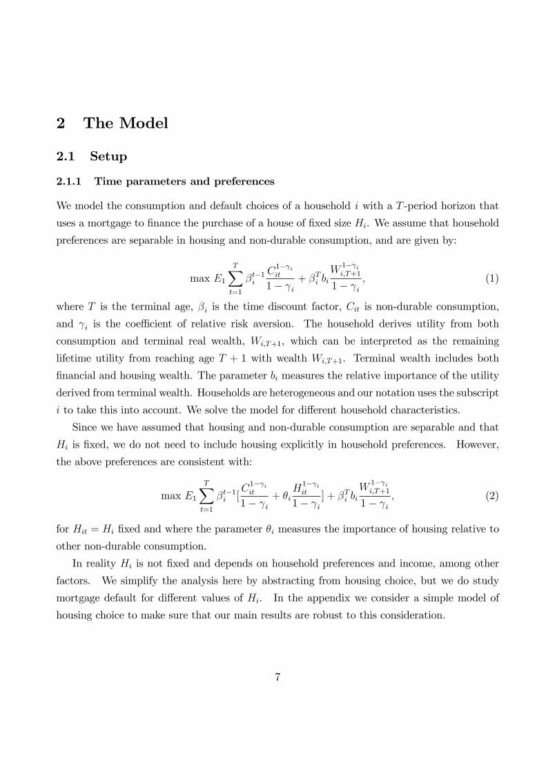
We model the consumption and default choices of a household i with a T -period horizon that
uses a mortgage to �nance the purchase of a house of �xed size Hi. We assume that household
preferences are separable in housing and non-durable consumption, and are given by:
max E1
TXt=1
�t�1i
C1� iit
1� i+ �Ti bi
W1� ii;T+1
1� i; (1)
where T is the terminal age, �i is the time discount factor, Cit is non-durable consumption,
and i is the coe¢ cient of relative risk aversion. The household derives utility from both
consumption and terminal real wealth, Wi;T+1, which can be interpreted as the remaining
lifetime utility from reaching age T + 1 with wealth Wi;T+1. Terminal wealth includes both
�nancial and housing wealth. The parameter bi measures the relative importance of the utility
derived from terminal wealth. Households are heterogeneous and our notation uses the subscript
i to take this into account. We solve the model for di¤erent household characteristics.
Since we have assumed that housing and non-durable consumption are separable and that
Hi is �xed, we do not need to include housing explicitly in household preferences. However,
the above preferences are consistent with:
max E1
TXt=1
�t�1i [C1� iit
1� i+ �i
H1� iit
1� i] + �Ti bi
W1� ii;T+1
1� i; (2)
for Hit = Hi �xed and where the parameter �i measures the importance of housing relative to
other non-durable consumption.
In reality Hi is not �xed and depends on household preferences and income, among other
factors. We simplify the analysis here by abstracting from housing choice, but we do study
mortgage default for di¤erent values of Hi. In the appendix we consider a simple model of
housing choice to make sure that our main results are robust to this consideration.
7

2.1.2 Interest and in�ation rates
Nominal interest rates are variable over time. This variability comes from movements in both
the expected in�ation rate and the ex-ante real interest rate. We use a simple model that
captures variability in both these components of the short-term nominal interest rate.
We write the nominal price level at time t as Pt, and normalize the initial price level P1=1.
We adopt the convention that lower-case letters denote log variables, thus pt � log(Pt) and thelog in�ation rate �t = pt+1�pt. To simplify the model, we abstract from one-period uncertaintyin realized in�ation; thus expected in�ation at time t is the same as in�ation realized from t to
t+1. While clearly counterfactual, this assumption should have little e¤ect on our results since
short-term in�ation uncertainty is quite modest. We assume that expected in�ation follows an
AR(1) process. That is,
�t = ��(1� ��) + ���t�1 + �t; (3)
where �t is a normally distributed white noise shock with mean zero and variance �2� . The
ex-ante real interest rate also follows an AR(1) process. The expected log real return on a
one-period bond, r1t = log(1 +R1t), is given by:
r1t = �r(1� �r) + �rr1;t�1 + "t; (4)
where "t is a normally distributed white noise shock with mean zero and variance �2".
The log nominal yield on a one-period nominal bond, y1t = log(1 + Y1t); is equal to the log
real return on a one-period bond plus expected in�ation:
y1t = r1t + �t: (5)
We let expected in�ation be correlated with the ex-ante real interest rate and denote the
coe¢ cient of correlation by ��;r.
2.1.3 Labor income and taxation
Household i is endowed with stochastic gross real labor income in each period t, Lit; which
cannot be traded or used as collateral for a loan. As usual we use a lower case letter to denote
8

the natural log of the variable, so lit � log(Lit). The household�s log real labor income is
exogenous and is given by:
lit = fi(t; Zit) + vit + !it; (6)
where fi(t; Zit) is a deterministic function of age t and other individual characteristics Zit, and
vit and !it are random shocks. In particular, vit is a permanent shock and assumed to follow a
random walk:
vit = vi;t�1 + �it; (7)
where �it is an i.i.d. normally distributed random variable with mean zero and variance �2�i :
The other shock represented by !it is transitory and follows an i.i.d. normal distribution with
mean zero and variance �2!i. Thus log income is the sum of a deterministic component and two
random components, one transitory and one persistent.
We let real transitory labor income shocks, !it, be correlated with innovations to the sto-
chastic process for expected in�ation, �t, and denote the corresponding coe¢ cient of correlation
�!i;�. In a world where wages are set in real terms, this correlation is likely to be zero. If wages
are set in nominal terms, however, the correlation between real labor income and in�ation may
be negative. As before, we use the subscript i throughout to model the fact that households are
heterogenous in the characteristics of their labor income, including the variance of the income
shocks that they face.
We model the tax code in the simplest possible way, by considering a linear taxation rule.
Gross labor income, Lit, and nominal interest earned are taxed at the constant tax rate � . We
allow for deductibility of nominal mortgage interest at the same rate.
2.1.4 House prices and other housing parameters
We model house price variation as an aggregate process. Let PHt denote the date t real price of
housing, and let pHt � log(PHt ). We normalize PH1 = 1 so that H also denotes the value of the
house that the household purchases at the initial date. The real price of housing is a random
walk with drift, so real house price growth can be written as:
�pHt = g + �t; (8)
9

where g is a constant and � is an i.i.d. normally distributed random shock with mean zero and
variance �2�. We assume that the shock �t is uncorrelated with in�ation, so in our model housing
is a real asset and an in�ation hedge. It would be straightforward to relax this assumption.
We assume that innovations to the permanent component of the household�s real labor
income, �it, are correlated with innovations to real house prices, �t, and denote by ��i;� the
corresponding coe¢ cient of correlation. When this correlation is positive, states of the world
with high house prices are also likely to have high permanent labor income. We let innovations
to the real interest rate be correlated with house price shocks, denoted by �";�.
We assume that in each period homeowners must pay property taxes, at rate � p, proportional
to house value, and that property tax costs are income-tax deductible. In addition, homeowners
must pay a maintenance cost, mp, proportional to the value of the property. This can be
interpreted as the maintenance cost of o¤setting property depreciation. The maintenance cost
is not income-tax deductible.
2.1.5 Mortgage contracts
The household is not allowed to borrow against future labor income. Furthermore, the max-
imum loan amount is equal to the value of the house less a down-payment. Therefore initial
loan amount (Di1):
Di1 � (1� di)P1PH1 Hi (9)
where di is the required down-payment. We use a subscript i for the required down-payment to
allow for the possibility that it di¤ers across households. We simplify the model by assuming
that the household �nances the initial purchase of the house of size Hi with previously accu-
mulated savings and a nominal mortgage loan equal to the maximum allowed, of (1 � di)Hi.
(Recall that we have normalized PH1 and P1 to one.) The LTV and LTI ratios at mortgage
origination are therefore given by:
LTVi = (1� di) (10)
LTIi =(1� di)Hi
Li1; (11)
where Li1 denotes the level of household labor income at the initial date.
10

Required mortgage payments depend on the type of mortgage. We consider several alter-
native types, including FRMs, ARMs, and ARMs with a teaser rate.
Let Y i;FRMT be the interest rate that household i pays on a FRM with maturity T . It is
equal to the expected interest rate over the life of the loan, or the yield on a long-term bond,
plus an interest rate premium which depends on loan and borrower characteristics. The date t
real mortgage payment, MFRMit , is given by the standard annuity formula:
MFRMit =
(1� di)Hi
��Y i;FRMT
��1��Y i;FRMT (1 + Y i;FRM
T )T��1��1
Pt: (12)
A distinctive feature of the US mortgage market is that FRMs come with a re�nancing
option that we model. More precisely, if households take out FRMs when interest rates are
high, and rates subsequently decline, then households who have the required level of positive
home equity, di, may decide to re�nance the loan and take advantage of the lower interest rates.
We assume that re�nancing costs are equal to a proportion cr of loan amount. We also assume
that households re�nance into a FRM with remaining maturity T � tr + 1, where tr denotes
the period of the re�nancing. More precisely, we assume that households re�nance into the
contract and the borrowing position that they would have been in period tr, had the interest
rates at the time that the loan began been lower.6
Let Y i;ARM1t be the one-period nominal interest rate on an ARM taken out by household i,
and let DARMit be the nominal principal amount outstanding at date t. The date t real mortgage
payment, MARMit , is given by:
MARMit =
Y i;ARM1t DARM
it +�DARMi;t+1
Pt; (13)
where �DARMi;t+1 is the component of the mortgage payment at date t that goes to pay down
principal rather than pay interest. We assume that for the ARM the principal loan repayments,
�DARMi;t+1 , equal those that occur for the FRM. This assumption simpli�es the solution of the
model since the outstanding mortgage balance is not a state variable.
6This simpli�es the numerical solution of the problem since we only need to solve the model for the di¤erent
possible levels of initial interest rates, sequentially, starting with the lowest, and using the value function as an
input into the problem when initial interest rates are higher. We give further details on the numerical solution
in section 2.2.
11
The date t nominal interest rate for the ARM is equal to the short rate plus a constant
premium:
Y i;ARM1t = Y1t + i;ARM : (14)
where the mortgage premium i;ARM compensates the lender for the prepayment and default
risk of borrower i. In the case of an ARM with a teaser rate, the mortgage premium is set to
zero for one initial period.
For a FRM the interest rate is �xed and equals the average interest rate over the loan ma-
turity (the average zero-coupon bond yield for that maturity under the expectations hypothesis
of the term structure) plus a premium i;FRM . In addition to prepayment and default risk, the
FRM premium compensates the lender for the interest rate re�nancing option that borrowers
receive. At times when the one-year yield is low (high), the term structure is upward (down-
ward) sloping, and long-term rates are higher (lower) than short-term rates. As previously
noted, we assume that mortgage interest payments are deductible at the income tax rate � .
2.1.6 Mortgage default and home rental
In each period the household decides whether or not to default on the mortgage loan. The
household may be forced to default because it has insu¢ cient cash to meet the mortgage
payment. However, the household may also �nd it optimal to default, even if it has the cash
to meet the payment.
We assume that in case of default, a mortgage lender has no recourse to the household�s
�nancial savings or future labor income. The mortgage lender seizes the house, the household is
excluded from credit markets, and since it cannot borrow the funds needed to buy another house
it is forced into the rental market for the remainder of the time horizon. These assumptions
simplify a complex reality. In the US the rules regarding recourse vary across state. In some
states home mortgages are explicitly non-recourse, whereas in others recourse is allowed but
onerous restrictions on de�ciency judgements render many loans e¤ectively non-recourse.7 In
7Ghent and Kudlyak (2011) use variation in state laws to empirically evaluate the impact of recourse on
default decisions. Li, White, and Zhu (2010) argue that US bankruptcy reform in 2005 a¤ected mortgage
default by making it harder for homeowners to use bankruptcy to reduce unsecured debt. See also Chatterjee
and Eyigungor 2009 and Mitman 2011, who solve equilibrium models of the macroeconomic e¤ects of bankruptcy
12

addition, defaulting households in the US are excluded from credit markets for a period of
time but not permanently. To understand the e¤ect of recourse, in the appendix we consider
a variation of our model in which lenders can seize borrowers�current �nancial assets in the
event of default, but have no claim on their future labor income.
The rental cost of housing equals the user cost of housing times the value of the house
(Poterba 1994, Diaz and Luengo-Prado 2008). That is, the date t real rental cost Uit for a
house of size Hi is given by:
Uit = [Y1t � Et[exp(�pHt+1 + �t)� 1] + � p +mp]PHt Hi; (15)
where Y1t is the one-period nominal interest rate, Et[exp(�pHt+1+ �1t)� 1] is the expected one-period proportional nominal change in the house price, and � p and mp are the property tax rate
and maintenance costs, respectively.8 This formula implies that in our model the rent-to-price
ratio varies with the level of interest rates.9
Relative to owning, renting is costly for two main reasons. First, homeowners bene�t from
the income-tax deductibility of mortgage interest and property taxes, without having to pay
income tax on the implicit rent they receive from their home occupancy. Second, owning
provides insurance against future �uctuations in rents and house prices (Sinai and Souleles,
2005). When permanent income shocks are positively correlated with house price shocks,
however, households have an economic hedge against rent and house price �uctuations even if
they are not homeowners.
We assume that in case of default the household is guaranteed a lower bound of X in
per-period cash-on-hand, which can be viewed as a subsistence level. This assumption can be
motivated by the existence of social welfare programs, such as means-tested income support.
In terms of our model it implies that consumption and default decisions are not driven by the
probability of extremely high marginal utility, which would be the case for power utility if there
was a positive probability of extremely small consumption.
laws and foreclosure policies.8To simplify we assume that maintenance costs are similar for homeowners and for rental properties. Al-
ternatively, we could have reasonably assumed that homeowners take better care of the properties, thereby
reducing maintenance expenses.9Campbell, Davis, Gallin, and Martin (2009) provide an empirical variance decomposition for the rent-to-
price ratio.
13

2.1.7 Early mortgage termination and home equity extraction
We model several potential sources of early mortgage termination. As previously mentioned,
we allow FRM borrowers to take advantage of a decrease in interest rates by re�nancing their
mortgage. In addition, we allow households who have accumulated positive home equity to sell
their house, repay the outstanding debt, and move into rental accommodation. The house sale
is subject to a realtor�s commission, a fraction c of the current value of the property. In this
way, albeit at a cost, households are able to access their accumulated housing equity, and use
it to �nance non-durable consumption. We interpret this event as a cash-out prepayment.
Ideally, in addition to cash-out prepayment, we would like to explicitly model other ways
in which households can draw down their accumulated home equity, for example using second
mortgages or home equity lines of credit. Home equity extraction can play an important
role in consumption smoothing and can have macroeconomic implications (Chen, Michaux,
and Roussanov 2013). Unfortunately this would increase the already large number of state
variables in our model, so we leave this topic for future research.
In addition to the above endogenous sources of mortgage termination, we model exogenous
random mortgage termination by assuming that in each period, with probability 'it, borrowers
are forced to move, in which case they sell the house, repay the principal outstanding, and move
into the rental market. If a household is hit with a moving shock at a time of negative home
equity, the household defaults on the loan. We allow for the possibility that negative home
equity creates a �lock-in�e¤ect, by letting the probability of a forced move be a lower value
'0it when home equity is negative.
2.1.8 Financial institutions
We assume a competitive market for mortgage providers. In addition, we assume that �nancial
institutions are able to screen borrowers and learn their characteristics. Therefore, the mortgage
premium that they will require for each contract will in equilibrium re�ect the probability of
prepayment, default and the expected losses given default of the speci�c borrower.10
10Since default and prepayment decisions depend on interest rates and mortgage premia, which also a¤ect
lenders�expected pro�ts, this requires, for each borrower type and mortgage contract, solving several iterations
of our model to �nd a �xed point. We give further details in Section 2.2.
14
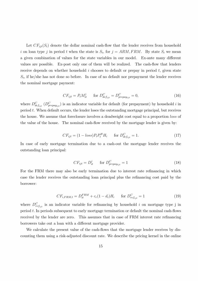
Let CFijt(St) denote the dollar nominal cash-�ow that the lender receives from household
i on loan type j in period t when the state is St, for j = ARM;FRM . By state St we mean
a given combination of values for the state variables in our model. Ex-ante many di¤erent
values are possible. Ex-post only one of them will be realized. The cash-�ow that lenders
receive depends on whether household i chooses to default or prepay in period t, given state
St, if he/she has not done so before. In case of no default nor prepayment the lender receives
the nominal mortgage payment:
CFijt = PtMjit for DC
defijt= DC
prepayijt= 0; (16)
where DCdefijt
(DCprepayijt
) is an indicator variable for default (for prepayment) by household i in
period t. When default occurs, the lender loses the outstanding mortgage principal, but receives
the house. We assume that foreclosure involves a deadweight cost equal to a proportion loss of
the value of the house. The nominal cash-�ow received by the mortgage lender is given by:
CFijt = (1� loss)PtPHt Hi for DC
defijt= 1: (17)
In case of early mortgage termination due to a cash-out the mortgage lender receives the
outstanding loan principal:
CFijt = Djit for DC
prepayijt= 1 (18)
For the FRM there may also be early termination due to interest rate re�nancing in which
case the lender receives the outstanding loan principal plus the re�nancing cost paid by the
borrower:
CFi;FRM;t = DFRMit + cr(1� di)Hi for DC
refijt= 1 (19)
where DCrefijt
is an indicator variable for re�nancing by household i on mortgage type j in
period t. In periods subsequent to early mortgage termination or default the nominal cash-�ows
received by the lender are zero. This assumes that in case of FRM interest rate re�nancing
borrowers take out a loan with a di¤erent mortgage provider.
We calculate the present value of the cash-�ows that the mortgage lender receives by dis-
counting them using a risk-adjusted discount rate. We describe the pricing kernel in the online
15

appendix (Campbell and Cocco 2014). Let PV1[CFijt](S1; S2; :::; St) denote the present value
(at the initial date) of the period t cash-�ow for loan type j taken out by household i. This
present value depends not only on the value of the date t state variables, but also on the value
of the state variables in previous periods since they a¤ect the rate that is appropriate to dis-
count the pro�ts.11 We scale the present value of the sum of the cash-�ows by loan amount to
calculate risk-adjusted pro�tability:
PRij(S) =
PTt=1 PV1[CFijt](S1; S2; :::; St)
(1� di)Hi
(20)
where S = [S1; S2; :::; ST ]. This gives us a measure of the return on each loan type, j =
ARM;FRM , for a given borrower type i, and for a given realization of the state variables. If
at the initial date we take expectations across all possible realizations of the state variables:
PRij(S1) = E1[PRij(S)] (21)
we obtain a measure of expected pro�tability of mortgage loan type j to borrower type i
conditional on the values for the state variables at the time that the mortgage is taken out.
These pro�tability calculations do not subtract administrative expenses, and should be
interpreted accordingly. Computationally it would be straightforward to subtract expenses
when calculating the pro�ts of mortgage providers, but one would need to specify the type of
expenses (per period or up front, �xed or as a proportion of the loan value).
2.2 Model summary and solution
2.2.1 Model summary
The state variables of the household�s problem are age (t), cash-on-hand (Xit), whether the
household has previously terminated the mortgage through prepayment or default or not
(DStermijt
, equal to one if previous prepayment or default and zero otherwise), real house prices
(PHt ), the nominal price level (Pt), in�ation (�t), the real interest rate (r1t), and the level of
permanent income (vit). For the FRM there is an additional state variable, whether the house-
11Only a subset of the state variables will a¤ect the discount rate, namely the aggregate variables in the model
(real interest rates, in�ation rate, and house prices).
16

hold has previously re�nanced the loan or not (DSrefijt
, equal to one if previous re�nance and
zero otherwise).
The choice variables are consumption (Cit), whether to default on the mortgage loan if no
default has occurred before (DCdefijt
, equal to one if the household i chooses to default on loan
j in period t and zero otherwise), and in the case of positive home equity whether to prepay
(DCprepayijt
, equal to one if the household chooses to prepay the mortgage in period t and zero
otherwise). For the FRM there is an additional choice variable, of whether to re�nance the loan
(DCrefijt
, equal to one if the household i chooses to re�nance the mortgage in period t and zero
otherwise).
In all periods before the last, if the household has not defaulted on or terminated its mort-
gage, its cash-on-hand evolves as follows for the case of an ARM:
Xji;t+1 = (Xit�Cit)
(1 + Y1t(1� �))
(1 + �t)�M i
it�(mp+� p)PHt Hi+Li;t+1(1��)+
Y ij1tDt�
Pt+� pP
Ht Hi� ;
(22)
for j = ARM . Savings earn interest that is taxed at rate � . Next period�s cash-on-hand is
equal to savings plus after-tax interest, minus real mortgage payments (made at the end of the
period), minus property taxes and maintenance expenses, plus next period�s labor income and
the tax deduction on nominal mortgage interest and on property taxes.
The equation describing the evolution of cash-on-hand for the FRM in periods in which
there is no re�nance is similar, except that the mortgage interest tax deduction is calculated
using the interest rate on that mortgage. In periods in which the FRM is re�nanced we need to
subtract the re�nancing cost and an amount equal to the di¤erence between the loan amount
on the new loan and the amount outstanding on the re�nanced loan.12
If the household has defaulted on or prepaid its mortgage and moved to rental housing, the
evolution of cash-on-hand is given by:
XRenti;t+1 = (Xit � Cit)
(1 + Y1t(1� �))
(1 + �t)� Uit + Li;t+1(1� �): (23)
where Uit denotes the date t real rental payment.
12The speed at which FRM principal is repaid depends on the initial interest rate. We take this di¤erence
into account when the loan is re�nanced.
17

Terminal, i.e. date T + 1, wealth is given by:
W ji;T+1 =
PT+1Xi;T+1 + PT+1PHT+1Hi
PCompositeT+1
; for j = ARM;FRM and DtermSij;T+1 = 0 (24)
WRenti;T+1 =
PT+1Xi;T+1
PCompositeT+1
; for DtermSij;T+1 = 1: (25)
If the household has not previously defaulted or terminated the mortgage contract, terminal
wealth is equal to �nancial wealth plus housing wealth. In the rental state, households only
have �nancial wealth at the terminal date.
Households derive utility from real terminal wealth, so that in all of the above cases nominal
terminal wealth is divided by a composite price index, denoted by PCompositeT+1 . This index is
given by:
PCompositeT+1 = [(PT+1)1� 1
i + �1 ii (PT+1P
HT+1)
1� 1 i ]
i i�1 (26)
where recall that i is the coe¢ cient of relative risk aversion and �i measures the preference for
housing relative to other goods in the preference speci�cation (2). The above composite price
index is consistent with our assumptions regarding preferences (Piazzesi, Schneider, and Tuzel
2007). The fact that nominal terminal wealth is scaled by a price index that depends on the
price of housing implies that even in the penultimate period homeownership serves as an hedge
against house price �uctuations (Sinai and Souleles 2005). The larger is �i the stronger is such
a hedging motive for homeownership.
2.2.2 Solution technique
Our model cannot be solved analytically. The numerical techniques that we use for solving it
are standard. Since the mortgage premium depends on mortgage type, borrower characteristics,
and the initial values of the aggregate state variables, we solve the model separately for each of
these cases. Recall that we have normalized the initial price level and house prices to one, so
that as far as the aggregate variables are concerned, we need to calculate the mortgage premium
for di¤erent initial levels of the in�ation and real interest rates.
18

The expected risk-adjusted pro�tability of each mortgage contract depends on the mortgage
premium, which a¤ects the default and prepayment decisions of borrowers, which in turn a¤ect
the expected risk-adjusted pro�tability of the loan. Therefore, for each case, we need to solve
several iterations of our model to �nd a �xed point. We do so using a grid for mortgage premia
with steps of �ve basis points. More precisely, we start by making a guess for the mortgage
premium, and then solve the borrower�s problem given that premium. Once we have the
borrower�s optimal decisions we use the transition probabilities and pricing kernel to calculate
expected risk-adjusted pro�tability. We then iterate: if the expected risk-adjusted pro�tability
is too high (low) we decrease (increase) the mortgage premium and re-solve the household�s
problem.
For each possible mortgage premium, we solve the borrower�s problem by discretizing the
state space and using backwards induction starting from period T + 1. The shocks are ap-
proximated using Gaussian quadrature, assuming two possible outcomes for each of them.
This simpli�es the numerical solution of the problem since for each period t we only need to
keep track of the number of past high/low in�ation, high/low permanent income shocks, and
high/low house price shocks to determine the date t price level, permanent income, and house
prices. For each combination of the state variables, we optimize with respect to the choice
variables. We use cubic spline or, in the areas in which there is less curvature in the value
function, linear interpolation to evaluate the value function for outcomes that do not lie on the
grid for the state variables. In addition, we use a log scale for cash-on-hand. This ensures that
there are more grid points at lower levels of cash-on-hand.
To handle the re�nancing option for FRMs, we solve the model sequentially, starting with
the lowest level of initial interest rates, and save the value function. We then use this value
function, in each period t subsequent to mortgage origination, as an input for the borrower�s
re�nancing decision in the solution for the case of higher initial interest rates.
2.3 Parameterization
2.3.1 Time and preference parameters
In order to parameterize the model we assume that each period corresponds to one year. We
set the initial age to 30 and the terminal age to 50. Thus mortgage maturity is 20 years. In the
19

baseline parameterization we set the discount factor � equal to 0.98 and the coe¢ cient of relative
risk aversion equal to 2. The parameter � that measures the preference for housing relative
to other consumption is set to 0:3. But we recognize that there is household heterogeneity
with respect to preference and other parameters, so that we solve the model for alternative
parameter values. The parameter that measures the relative importance of terminal wealth, b,
is assumed to be equal to 400. This is large enough to ensure that households have an incentive
to save, and that our model generates reasonable values for wealth accumulation. These time
and preference parameters are reported in the �rst panel of Table 1.
2.3.2 Interest and in�ation rates
We use data from the Livingston survey of in�ation expectations to parameterize the stochastic
process for expected in�ation (median one-year forecast, sample period 1987 to 2012). We
obtain information on 1-year nominal bond yields from the Federal Reserve and calculate the
expected 1-year real interest rate by de�ating the nominal yield by expected in�ation. The
estimated parameters for the AR(1) processes for the logarithm of expected in�ation and for
the logarithm of the expected real rate are reported in the second panel of Table 1. The implied
half-life of expected in�ation shocks is 6 years, while the half-life for real rate shocks is 3.6 years.
2.3.3 Labor income
We use data from the Panel Study of Income Dynamics (PSID) for the years 1970 to 2005
to calibrate the labor income process. Our income measure is broadly de�ned to include total
reported labor income, plus unemployment compensation, workers compensation, social security
transfers, and other transfers for both the head of the household and his spouse. We use such
a broad measure to implicitly allow for the several ways that households insure themselves
against risks of labor income that is more narrowly de�ned. Labor income was de�ated using
the consumer price index.
It is widely documented that income pro�le varies across education attainment (see for
example Gourinchas and Parker, 2002). To control for this di¤erence, following the existing
literature, we partition the sample into three education groups based on the educational attain-
ment of the head of the household. For each education group we regress the log of real labor
20

income on age dummies, controlling for demographic characteristics such as marital status and
household size, and allowing for household �xed e¤ects. We use this smoothed income pro�le
to calculate, for each education group, the average household income for an head with age 30
and the average annual growth rate in household income from ages 30 to 50. The estimated
real labor income growth rate for households with a high-school degree is 0.8 percent, and we
use this value in the benchmark case. The assumption of a constant income growth rate is a
simpli�cation of the true income pro�le that makes it easier to carry out comparative statics
and to investigate the role of future income prospects on the default decision.
We use the residuals of the above panel regressions to estimate labor income risk. In order
to mitigate the e¤ects of measurement error on estimated income risk, we have winsorized
the income residuals at the 5th and 95th percentiles. We follow the procedure of Carroll
and Samwick (1997) to decompose the variance of the winsorized residuals into transitory
and permanent components. The estimated parameter values reported in the third panel of
Table 1 should be interpreted as possible parameter values. Households are heterogenous in
the characteristics of their labor income, so that we solve our model for alternative parameter
values for expected labor income growth and income risk.
2.3.4 House prices
We use two di¤erent data sources to parameterize the parameters of the house price process,
namely PSID data and Case-Shiller house price indices. The advantage of the PSID is that
it contains both house price and labor income information. However, annual data which we
need to calculate annual house price returns are only available until 1997. Furthermore, PSID
house prices are self-reported and vulnerable to measurement error. We obtain real house
prices by dividing self-reported house prices by the consumer price index. House price changes
are calculated as the �rst di¤erence of log real house prices, for individuals who are present in
consecutive annual interviews, and who report not having moved since the previous year.
In order to address the issue of measurement error, and parallel to our treatment of labor
income, we have winsorized the logarithm of real house price changes at the 5th and 95th
percentiles (-36.6 and 40.3 percent, respectively). We use the winsorized data to calculate the
expected value and the standard deviation of real house price changes, which are equal to 1:6%
and 16:2%, respectively. In our baseline exercise we use these estimated values, but we consider
21

alternative parameterizations.
We use PSID household level data to estimate the correlation between labor income shocks
and house price shocks. In order to do so we �rst calculate:
�(lit ��f it) = [lit ��f (t; Zit)]� [li;t�1 ��f (t� 1; Zi;t�1)] = �it + !it � !i;t�1; (27)
where the symbol �f denotes the predicted regression values. We estimate a correlation between
(27) and the �rst di¤erences in log house prices, �t, that is positive and statistically signi�cant,
and equal to 0.037. Under the model assumption that temporary labor income shocks, !it, are
serially uncorrelated and uncorrelated with house price shocks, this value implies a correlation
between permanent labor income shocks, �it, and house price shocks, �t, equal to 0.191. This
value re�ects the fact that a signi�cant component of the innovations to permanent labor income
shocks is idiosyncratic (and therefore uncorrelated with house prices).
We also use the S&P/Case-Shiller 10-city composite home price index to parameterize the
model. The sample period is 1987 to 2012. We are particularly interested in the relation
between house prices and real interest rates. As before, we de�ate the house price index by the
consumer price index and calculate the logarithm of annual real house price growth. The mean
log real house price growth is higher than that estimated in the PSID data, equal to 0.005,
due to the di¤erences in the period covered. The standard deviation of log real house price
growth is somewhat lower than in PSID data, equal to 0.09. We estimate a positive correlation
between innovations to the logarithm of real interest rates and log real house price returns,
equal to 0.38, with a p-value of 0.07. We parameterize the model using a somewhat lower value
of 0.30. We set the remaining model correlations to zero.13
The S&P/Case-Shiller composite house price index is less volatile than self-reported house
prices from the PSID, because idiosyncratic house price variation diversi�es away in the compos-
ite index.14 Our model abstracts from idiosyncratic house price variation, but nonetheless we
calibrate it using an estimate of total house price volatility since all movements in house prices,
13We have estimated the correlation between log real house price returns and expected in�ation, but the
estimated value was not signi�cantly di¤erent from zero.14This diversi�cation e¤ect is also visible in data on median US house prices from the Monthly Interest Rate
Survey. Over the period 1991 to 2007 the average growth rate in real (nominal) house prices was 1.2 (3.9)
percent, with a standard deviation of only 4.8 percent.
22

not just aggregate movements, a¤ect homeowners�incentives to default on their mortgages.
2.3.5 Tax rates and other parameters
We follow Himmelberg, Mayer, and Sinai (2005) in setting the values for the tax rates. More
precisely, we set the income tax rate, � , equal to 0:25, the property tax rate � p equal to 0:015,
and the property maintenance expenses, mp, equal to 0:025. In addition we assume that a house
sale is subject to a realtor commission, tc, equal to 6 percent of the value of the house, which
is a fairly standard value. We set the lower bound on (real) cash-on-hand to one thousand
dollars. We set the exogenous probability of a house move for borrowers with positive home
equity to 0.04. Chan (2001) estimates that an increase in LTV to over 95% would result in a
moving probability that is 20% of the original. Therefore in case of negative home equity we
set the exogenous moving probability equal equal to 0.008.
2.3.6 Loan parameters
We consider alternative values for the downpayment/initial LTV and LTI, but in order to
facilitate the discussion we refer to the case of a LTV ratio of 0.9 and a LTI equal to 4.5 as
the baseline. We set the costs of re�nancing the FRM contract tr equal to one percent of the
loan amount. The credit risk premium on each of the mortgage loans, ij, where i denotes the
borrower and j = FRM;ARM is determined endogenously.
2.4 Simulated data
We solve the model separately for each mortgage type, borrower characteristics, and combina-
tion of the initial values for the aggregate variables. Since we have normalized the initial price
level and real house prices to one, the aggregate variables we need to consider are expected
in�ation and real rate. In the numerical solution we have assumed two possible states for each
of these, which implies four di¤erent values for the initial 1-year nominal rates. For each case,
once we �nd a �xed point for the problem, we use the optimal policy functions to generate
simulated data.
Agents in our model are subject to both aggregate and idiosyncratic shocks. Aggregate
shocks are to real house prices, the in�ation rate, and real interest rates. Idiosyncratic shocks
23

are innovations to the permanent component of the labor income process (which also have an ag-
gregate component since they are positively correlated with house price shocks) and temporary
labor income shocks.
We �rst generate one realization for the aggregate shocks and then for this realization we
generate realizations for the shocks to the labor income process for �fty individuals. We use
the model policy functions, the one path for the aggregate variables and the individual income
shocks to simulate optimal consumption, prepayment, re�nancing and default behavior for these
�fty individuals. We then repeat the process for a total of eight hundred di¤erent paths for
the aggregate variables, and for �fty individuals for each of these paths. This yields, for each
initial value for the aggregate variables, mortgage and borrower type, a total of forty thousand
di¤erent paths. We use the same realizations for the shocks to simulate consumption and
default behavior for each of the di¤erent mortgage types that we study.
To understand the basic properties of the simulated data, in Figure A.1 of the online ap-
pendix we plot the age pro�les of cross-sectional average real gross income, consumption and
cash-on-hand. Real consumption is on average considerably lower than real gross income. The
reason is that part of gross income must be paid in taxes, and the individual must also make
mortgage payments and other housing related expenditures such as property taxes and main-
tenance expenses. Part of income is also saved.15
In the next section we use the simulated data to predict unconditional default, prepayment,
and re�nancing probabilities, that is probabilities calculated across the di¤erent paths for the
aggregate and idiosyncratic variables in the model. These are expected probabilities calculated
at the initial date. Ex-post only one of the many possible paths for the aggregate variables will
be realized. Section 4 studies probabilities conditional on a speci�c path. This analysis allows
us to determine the relative contributions of aggregate and idiosyncratic shocks to default. Of
particular interest will be a path of low interest rates and declining house prices in which we
try to replicate the economic conditions following the recent U.S. crisis.
15Although not completely visible in Figure A.1, there is a slight decline in the average real consumption
pro�le with age. This happens for two main reasons. First, this is an average pro�le across many aggregate
states, including those with declining house prices (and income). Second, we have estimated an average growth
rate of house prices higher than labor income (not in logs, but in levels), and house price increases also drive
up housing-related expenses.
24

3 Unconditional Default Rates
3.1 Mortgage default triggers for ARMs and FRMs
We are interested in determining what triggers default in our model. We focus our attention
on home equity and the ratio of mortgage payments to income. The empirical literature on
mortgage default has emphasized the importance of home equity for the default decision (see
for example Deng, Quigley, and Van Order 2000, or more recently Foote, Gerardi, and Willen
2008 and Bajari, Chu, and Park 2009).
To measure home equity, we calculate for each household i and for each date t the current
outstanding debt as a fraction of current house value:
LTVijt =Dijt
PtPHt Hit
(28)
where Dijt denotes the loan principal amount outstanding on mortgage j at date t, Pt denotes
the price level, and PHt the real price of housing. A value of LTVijt above one corresponds to
negative home equity. Equation (28) shows that negative home equity tends to occur for a
particular combination of the state variables: declines in house prices, when the price level is
low, and at times when there are large mortgage balances outstanding (early in the life of the
loan).16
In Figure 2 we plot default probabilities for ARMs, conditional on the level of negative
equity. These probabilities are shown as solid lines in four alternative cases. In panel A we
plot the results for the baseline level of income risk (a standard deviation of temporary income
shocks of 0.225), and in panel B for a higher level of income risk (a standard deviation of
0.35). For each panel, the left �gure shows the results for a low initial interest rate (de�ned
as the lowest interest rate in our discretization of the model), while the right �gure shows the
results for a high initial interest rate (de�ned as the second highest discrete interest rate, since
the highest rate is extreme and rarely observed). We use these two levels of interest rates
16In our model the probability of negative equity �rst rises, as negative shocks have time to erode initially
positive home equity, then declines later in the life of the mortgage, as the loan is repaid, as in�ation erodes
the value of the outstanding nominal debt, and as real house prices (on average) increase. This explains why
most defaults occur in the �rst half of the life of the loan. Schwartz and Torous (2003) have found in regressions
aimed at explaining default rates that the age of the mortgage plays an important role.
25

throughout our presentation of results to illustrate the properties of the model.
The default probabilities in Figure 2 are calculated using one observation per mortgage, so
that for those households who choose never to default, in spite of being faced with negative
equity, we calculate these probabilities using the lowest level of equity that the household faces
during the life of the mortgage. This is similar to the calculations carried out by Bhutta, Dokko,
and Shan (2010) who study default rates for non-prime borrowers from Arizona, California,
Florida, and Nevada.
Figure 2 shows that few households default at low levels of negative home equity. For most
of the cases considered the probability of default is less than ten percent for LTV�s up to 1.3.
Thus households only exercise their option to default when it is considerably in the money. This
prediction of our model is consistent with the evidence in Bhutta, Dokko, and Shan (2010), who
�nd that the median homeowner does not default until equity falls to -62 percent of their home�s
value, and Foote, Gerardi, and Willen (2008), who study one hundred thousand homeowners
in Massachusetts who had negative equity during the early 1990s, and �nd that fewer than ten
percent of these owners lost their home to foreclosure.
The prediction that borrowers do not default as soon as home equity becomes negative is a
prediction of all default models based on real option theory. A special feature of our model is
that the ratio of mortgage payments to household income (MTI) also plays an important role:
MTIijt =Mijt
Lit: (29)
At the most basic level this is illustrated by the fact that ARM default rates are higher for
borrowers with high labor income risk who take out ARMs at high initial rates (the bottom
right panel of Figure 2).
The bars in Figure 2 show, for each level of negative equity, the di¤erence in current MTI
between those households who choose to default and those who choose not to default. Focusing
�rst on the case of low income risk, at very low levels of negative home equity the few bor-
rowers who default do so because they are forced to move. This explains the fairly small (and
even slightly negative) di¤erences in MTI between the two groups of borrowers. When home
equity becomes more negative, and when initial interest rates are high (Panel A.2), the ratio of
mortgage payments to income becomes more important for the default decision. Its importance
is most visible in Panel B.2, where the combination of high initial rates and high income risk
26

leads households to endogenously default at relatively low levels of negative home equity, and
where there are large di¤erences in current MTI between defaulting and non-defaulting bor-
rowers. Large mortgage payments relative to household income, in the presence of borrowing
constraints and low savings, force a choice between severe consumption cutbacks and mortgage
default. Elul, Souleles, Chomsisengphet, Glennon and Hut (2010) provide empirical evidence
of the importance of liquidity considerations for mortgage default decisions.
The default probabilities in Figure 2 show that at high levels of negative home equity the
vast majority of borrowers decide to default. At these levels, wealth motives tend to be an
important determinant of default decisions. This is consistent with the empirical �ndings of
Haughwout, Okah, and Tracy (2010). They study mortgage re-default using data on subprime
mortgage modi�cations for borrowers who were seriously delinquent, and whose monthly mort-
gage payment was reduced as part of the modi�cation. They �nd that the re-default rate
declines relatively more when the payment reduction is achieved through principal forgiveness
as compared to lower interest rates. The empirical analysis of Doviak and MacDonald (2011)
also emphasizes the role of modi�cations that reduce loan balances in preventing default.17
In order to better understand the importance of wealth and cash-�ow motives for mortgage
decisions, Table 2 reports the means of several variables for ARM borrowers who choose to
default, for borrowers with negative home equity but who choose not to default, for borrowers
who choose to cash out, and for borrowers who take no action (whether or not they have
negative home equity). In this table, by contrast with Figure 2, each household-date pair is an
observation so any given mortgage is observed multiple times and possibly in multiple states.
As before, we report results for low and high initial interest rates, and for low and high
income risk. Across these four cases, we see that households with negative home equity who
default tend to have more negative home equity than those with negative home equity but
who choose not to default. In addition, households who choose to default are those with lower
income and larger mortgage payments relative to income. The larger MTIs are also the result
of higher nominal interest rates. The di¤erence in MTIs is larger when initial interest rates
and income risk are high: in this case the average MTI is equal to 0.40 for households who
default compared to an average MTI ratio of 0.34 for households with negative equity who
17Das (2011) and Foote, Gerardi, Goette, and Willen (2009) provide model-based analysis of mortgage mod-
i�cation.
27

choose not to default. Table 2 also reports the di¤erence between mortgage and rent payments
scaled by household income. For households signi�cantly underwater who choose to default,
that decision allows for a reduction in current expenditure of between 26 and 30 percent of
income (depending on the case considered).
These results illustrate the fact that in our model, default is driven by both wealth and
cash-�ow considerations. House price declines lead to situations of negative home equity. Those
households who face larger house price declines, at times when outstanding debt is large, are
more likely to default. Since house price shocks are correlated with permanent income shocks,
larger house price declines tend to be associated with larger decreases in household income.
This forces households to cut back on non-durable consumption. For ARMs such cutbacks are
more severe when interest rates are high, since they lead to an increase in mortgage payments.
This can be seen in Table 2, as the average level of consumption is lowest among high-income-
risk borrowers just prior to default (Panel B.2). The last row of each panel in Table 2 reports
probabilities of default. They are higher when income risk is higher, but the increase is more
pronounced for ARM loans taken at times when initial interest rates are high. Interestingly,
higher income risk means that borrowers default on average at lower LTVs.
Table 2 also characterizes those households who decide to access their home equity (cash-
out). Compared to no action, these households have on average accumulated more home equity,
mainly as a result of larger increases in house prices. Furthermore, they face higher interest
rates and higher mortgage payments relative to income, and have lower levels of income and
consumption prior to the decision to cash-out. This combination motivates their decision to
tap into their home equity. When income risk is higher, households on average tap into their
home equity at slightly higher LTVs.
Turning to �xed-rate mortgages, in Table 3, we see that when initial interest rates are low,
default rates for FRMs are lower than for ARMs. However, the reverse is true when initial
interest rates are high. The reason is simple. When initial interest rates are high, mortgage
providers must charge borrowers for the option to re�nance the loan. This increases the premium
and the average payments of FRMs. It makes them particularly expensive in scenarios of house
price declines and low interest rates. Negative home equity prevents borrowers from re�nancing
the loan, while low interest rates lead to a lower user cost of housing and lower rental payments
compared to mortgage payments. On the other hand, for ARMs default tends to occur when
28

nominal interest rates are high, since high interest rates lead to large mortgage payments.
Table 3 also reports summary statistics for those borrowers who decide to cash-out or to
re�nance their FRMs. The determinants of the decision to cash-out are similar to the ARM:
large house price increases, lower income, and higher mortgage payments to income motivate
borrowers to tap into their home equity. When initial interest rates are high, the probability
of early mortgage termination as a result of a cash-out is considerably smaller. The reason is
that the mortgage is more likely to be terminated as a result of an interest rate re�nancing.
Unsurprisingly, borrowers tend to re�nance when interest rates are low. Borrowers who face
higher income risk are more likely to default or cash-out, and less likely to terminate their loan
with a re�nancing.
3.2 Mortgage premia and pro�tability
Table 4 reports mortgage premia for the same two initial levels of one-year bond yields that we
used in Figure 2. The column �low initial yield�reports the results for the lowest level of interest
rates in our model, corresponding to a positively sloped term structure. The column �high initial
yield�reports results for the second highest level of initial interest rates, corresponding to an
almost �at term structure. Results for other levels of interest rates are reported in the online
appendix.
The mortgage premia reported in Table 4 are determined endogenously so that mortgage
providers are able to achieve risk-adjusted discounted pro�tability of ten percent.18 This is
gross pro�tability, before expenses incurred by banks, and expected at the initial date, i.e.
averaging across the di¤erent possible paths for the aggregate variables. Ex post, only one
of these aggregate paths will be realized. The table also reports conditional probabilities of
default, cash-out, and FRM re�nancing, and the pro�tability associated with each of these
cases (which is lowest in the event of default, intermediate for cash-out and FRM re�nancing,
and highest if none of these events occur).
Focusing �rst on the results for ARMs, we see that the required mortgage premium is
almost constant but slightly increasing in the level of initial interest rates. This pattern results
18We chose this level so as to quantitatively try to match the average premia observed in the data. We report
results for other levels of risk-adjusted pro�tability in section 3.5 and compare the model with the data in section
4.3.
29

from three o¤setting e¤ects. First, the ARM default probability declines with the level of
initial interest rates. Although high initial interest rates imply a high initial MTI ratio as
shown in the table, reducing mortgage a¤ordability, high initial rates and in�ation also imply
that outstanding nominal mortgage balances are eroded faster by in�ation, so households are
likely to have lower LTVs later in the life of the mortgage. For the baseline parameters the
latter e¤ect dominates (but in section 3.4 we will show that the mortgage a¤ordability e¤ect
dominates for households who face higher income risk, so that for these borrowers the default
probability increases with the level of initial interest rates). Second, the probability of ARM
cash-out increases with the level of initial interest rates. Third, the pro�ts generated by the
mortgage premium are discounted more heavily when interest rates are initially high. The �rst
e¤ect makes the ARM premium decrease with the level of initial interest rates, but the second
and third e¤ects make it increase, and these dominate in the benchmark case.
Panel B reports the results for FRMs. We report endogenously determined mortgage premia
calculated over two di¤erent benchmark yields. The �rst is the premium over the yield on a 20-
year zero coupon bond. The second is the premium over the yield on a 20-year annuity priced
using the initial term structure of interest rates. The latter is a more reasonable benchmark
since mortgages make constant payments like annuities, and therefore have lower duration than
zero-coupon bonds of the same maturity. For this reason we focus the discussion on annuity-
relative premia to capture the pure compensation that mortgage providers require for default,
prepayment, and re�nancing risk.
The required mortgage premium for FRMs increases with the level of initial yields much
more steeply than does the required mortgage premium for ARMs. The main reason is the
presence of the interest rate re�nancing option. A higher initial yield increases the value of this
option and probability that it will be exercised. Lenders must be compensated for re�nancing
risk through a higher mortgage premium. The increased premium in turn makes it more likely
that borrowers default when faced with negative home equity that prevents them from exercising
the option. This explains why default probabilities now increase with the level of initial rates,
from 0.034 to 0.051. Pro�tability in case of default is higher than for the ARM contract. This
is mainly due to the fact that FRM borrowers tend to default when interest rates are low, so
that the present value of the recovered house is higher. Also, higher initial interest rates mean
that FRMs are more likely to be terminated as a result of interest rate re�nancing and less
30

likely to be terminated as a result of borrowers wishing to tap into their home equity.
The last panel of Table 4 reports borrower welfare bene�ts for ARMs relative to FRMs.
These welfare bene�ts are calculated as consumption equivalent variations, or the percentage
of the (constant) consumption equivalent stream that individuals would be willing to give up
to have the ARM contract instead of the FRM contract. Therefore, these calculations also tell
us what the mortgage choices of individuals at the initial date would be. When initial rates
are low borrowers are less likely to prefer an ARM, but the di¤erence relative to the FRM, of
�0:12% is not large. When initial rates and mortgage payments to income are low borrowers
are better positioned to meet the relatively higher initial mortgage payments of FRMs. At the
same time, the likelihood that interest rates will increase is large, which reduces the appeal of
ARMs, and increases the incentives to lock-in the low initial rate. As initial interest rates and
the ratio of mortgage payments to income increase, borrowers become less willing to pay the
additional premium that FRMs require.
3.2.1 FRM re�nancing inertia
In our model households exercise the interest rate re�nancing option of FRMs optimally. At
higher levels of initial interest rates the value of the option is larger, which together with the
expectation of optimal household exercise, implies that mortgage providers require a very much
larger premium at origination. However, Miles (2004) and Campbell (2006) present evidence
that many households do not re�nance when it would be optimal to do so, so that there is some
degree of household re�nancing inertia. We evaluate, in the context of our model, the e¤ects of
such inertia on mortgage premia. We model inertia in a simple way, by assuming that in each
period there is a probability, pinertia, that households do not re�nance even though it would
be optimal to do so. If as a result of inertia households do not re�nance immediately, they
may do so in the following period provided that it still is optimal to re�nance and that they
do not su¤er from further inertia. Households are aware of their degree of inertia and make
consumption and mortgage decisions taking it into account. Mortgage providers are also aware
of the degree of household inertia and price mortgages accordingly.
The results for di¤erent levels of inertia are shown in Table 5. In the �rst column we report
the results for the lowest level of initial interest rates, for which the re�nancing option is not
relevant. In the columns to the right we report the results for high initial yield, for the baseline
31
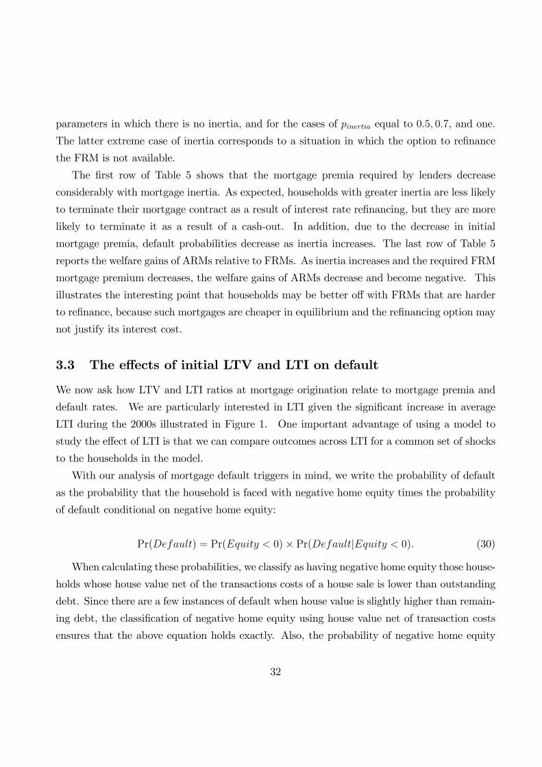
parameters in which there is no inertia, and for the cases of pinertia equal to 0:5; 0:7, and one.
The latter extreme case of inertia corresponds to a situation in which the option to re�nance
the FRM is not available.
The �rst row of Table 5 shows that the mortgage premia required by lenders decrease
considerably with mortgage inertia. As expected, households with greater inertia are less likely
to terminate their mortgage contract as a result of interest rate re�nancing, but they are more
likely to terminate it as a result of a cash-out. In addition, due to the decrease in initial
mortgage premia, default probabilities decrease as inertia increases. The last row of Table 5
reports the welfare gains of ARMs relative to FRMs. As inertia increases and the required FRM
mortgage premium decreases, the welfare gains of ARMs decrease and become negative. This
illustrates the interesting point that households may be better o¤ with FRMs that are harder
to re�nance, because such mortgages are cheaper in equilibrium and the re�nancing option may
not justify its interest cost.
3.3 The e¤ects of initial LTV and LTI on default
We now ask how LTV and LTI ratios at mortgage origination relate to mortgage premia and
default rates. We are particularly interested in LTI given the signi�cant increase in average
LTI during the 2000s illustrated in Figure 1. One important advantage of using a model to
study the e¤ect of LTI is that we can compare outcomes across LTI for a common set of shocks
to the households in the model.
With our analysis of mortgage default triggers in mind, we write the probability of default
as the probability that the household is faced with negative home equity times the probability
of default conditional on negative home equity:
Pr(Default) = Pr(Equity < 0)� Pr(DefaultjEquity < 0): (30)
When calculating these probabilities, we classify as having negative home equity those house-
holds whose house value net of the transactions costs of a house sale is lower than outstanding
debt. Since there are a few instances of default when house value is slightly higher than remain-
ing debt, the classi�cation of negative home equity using house value net of transaction costs
ensures that the above equation holds exactly. Also, the probability of negative home equity
32

is calculated as the probability that the borrower faces at least one period of negative equity
during the life of the mortgage.
The results are reported in Table 6. Panel A shows the results for ARMs, and Panel B for
FRMs, with a low initial interest rate scenario at the left and a high initial interest rate scenario
at the right. For each scenario, we consider three cases. In the �rst column we report the
results for the baseline case, with an LTV of 0.90 and an LTI of 4.5. The probability of negative
home equity tends to decline with the level of initial rates. There are two opposing e¤ects. The
higher the initial rates, the higher the proportion of mortgage payments that cover interest
payments, and the lower the initial reduction in principal outstanding. On the other hand,
higher initial expected in�ation and nominal interest rates mean that nominal house prices are
more likely to increase, which reduces the likelihood of negative home equity. Interestingly, we
see that the probability of default conditional on negative equity is higher for ARMs than for
FRMs for low initial rates, but that the reverse is true for high initial rates. For low initial rates,
the ARM borrowers who eventually default tend to be those who subsequently face house price
declines and higher interest rates. FRM borrowers who locked in a low rate at the initial date
are not as a¤ected by the subsequent increase in rates and are therefore less likely to default.
In the second column we report results for a lower LTI equal to 3.5. Focusing �rst on the
ARMwe see that default probabilities are now lower. The main reason is the lower probability of
default in case of negative equity, with a smaller e¤ect on the probability of negative equity. The
lower the initial LTI the lower are mortgage payments relative to household income, which makes
liquidity constraints less severe, and makes it less likely that households default when faced with
negative equity. Furthermore, due to the lower mortgage payments to income households in a
lower LTI loan have less of an incentive to tap into their home equity. The reduction in default
and cash-out probabilities contribute to a reduction in mortgage premia that is larger for a high
initial yield.
For the FRM contract, and similarly to the ARM contract, borrowers in lower LTI loans are
less likely to default or to wish to tap into their home equity. However, there is an additional
e¤ect: when initial interest rates are high borrowers are now much more likely to re�nance the
loan if interest rates subsequently decline, an event for which lenders must be compensated
ex-ante under the form of a higher mortgage premium. In spite of the increase in FRM premia
for high initial yields, the welfare gains of ARMs for lower LTI borrowers are lower than in the
33

baseline case. Lower LTIs and lower initial mortgage payments mean that households are less
borrowing constrained and they bene�t less from the relatively lower initial mortgage payments
to income of ARMs.
In the third column of each Table 6 scenario we study the e¤ects of a reduction in LTV
from 0.9 to 0.8. Unsurprisingly, a lower LTV reduces the probability of negative home equity.
Quantitatively, this leads to a very large reduction in the probability of default. Krainer, Leroy
and Mungpyung (2009) develop an equilibrium valuation model that emphasizes the role of the
initial LTV for mortgage default. The lower default rate means that the ARM premia required
by lenders are generally lower. We say generally because a lower LTV implies higher home
equity for households and increases the probability of early mortgage termination through a
cash-out. Since cash-out is unpro�table for mortgage lenders, a higher probability of cash-
out leads to an increase in premium that o¤sets the decrease due to the lower probability of
default. However, for the cases considered in Table 6, the reduction in default probability is
the dominant e¤ect.
For FRMs the reduction in LTV also leads to a reduction in default probabilities and
an increase in the probability of cash-out. In addition, there is a signi�cant decrease in the
probability that the loan will be re�nanced. The latter e¤ect explains why, when initial rates
are high, the reduction in the mortgage premia required by lenders when we move from a LTV
of 0.9 to 0.8 is larger for the FRM than the ARM contract. This di¤erential reduction also
explains the decrease in the welfare bene�ts of ARMs relative to FRMs.
The results in Table 6 show that there is a di¤erential sensitivity of default rates of FRMs and
ARMs to LTI and LTV ratios. On the one hand, default rates for FRMs decrease less with an
increase in LTI than do default rates for ARMs, particularly at low levels of initial interest rates.
On the other hand, default probabilities for FRMs are more sensitive to LTV than are default
probabilities for ARMs. This di¤erential sensitivity can be understood in light of our previous
analysis of default triggers. For ARMs a higher proportion of individuals default for cash-
�ow reasons. A higher LTI implies larger mortgage payments relative to income which makes
borrowing constraints more likely to bind. On the other hand, for FRMs, a higher proportion
of individuals default for wealth reasons. This makes default rates for these mortgages more
sensitive to the LTV ratio. This distinction between the cash-�ow risk of ARMs and the wealth
risk of FRMs has been emphasized by Campbell and Cocco (2003).
34

3.4 Borrower heterogeneity
In the previous sections we have studied mortgage default for di¤erent initial LTV and LTI
ratios, and for di¤erent mortgage types, but for �xed household preference parameters. In
reality borrowers are heterogenous, which has e¤ects on portfolio choice (Curcuru, Heaton,
Lucas, and Moore, 2010) and is also likely to a¤ect mortgage choice. With this in mind, in
this section we investigate further the e¤ects of household characteristics on mortgage premia,
default rates, and borrower welfare. Recall that we have assumed that banks can observe
household characteristics, and price loans accordingly.19
3.4.1 Labor income risk
Table 7 shows the results for the case in which borrowers face a higher standard deviation of
temporary labor income shocks, equal to 0.35 (in the column labelled higher). When labor
income risk is higher, ARM borrowers are more likely to default, in case house prices subse-
quently decline, or to cash-out, in case house prices subsequently increase. The increases in
the probabilities are larger when initial rates are high, and so is the additional ARM premia
that banks require to lend to riskier borrowers. Qualitatively, the e¤ects are similar for FRMs.
However, quantitatively there are some interesting di¤erences. For high initial rates the increase
in default probabilities and in mortgage premia is higher for FRMs than for ARMs. The addi-
tional mortgage premia that lenders require from riskier borrowers increase the average level of
mortgage payments. When initial rates are high, this a¤ects more FRM borrowers than ARM
borrowers, since the former need to meet on average higher initial mortgage payments, due to
re�nancing option which increases the premium on FRMs. This also explains why, when initial
interest rates are high, the bene�ts of ARMs relative to FRMs are larger for riskier borrowers
(Panel C).
In the last column of Table 7 we study the e¤ects of allowing labor income realization to
depend on the level of interest rates (correlated). More precisely, as in the case of higher income
risk we set the overall standard deviation of temporary labor income shocks equal to 0.35. In
19Furthermore, we assume that the pricing kernel is the the same as the one previously derived. The assump-
tion is that the representative agent has our baseline preferences and other parameters. It would be interesting
to investigate mortgage pricing for a population of heterogeneous households whose characteristics can only be
imperfectly observed by banks.
35

the higher income risk scenario the average level of log temporary income shocks is zero for
all levels of the short rate. In the correlated scenario, the average level of the log temporary
labor income shock is related to the level of interest rates. It is equal to -0.49 when one-year
yields are at their lowest level, it increases to -0.07 for the second lowest level of one-year yields,
followed by 0.07, and by 0.49. The motivation for this type of income risk is simple: interest
rates tend to be lower in recessions which reduce the labor income that some households receive.
Naturally, recessions a¤ect some workers more than others, so that the scenario with higher
income risk related to the short rate should not be seen as representative of the situation of all
borrowers.
Some interesting patterns emerge. First, the probabilities of default and of cash-out are
higher for lower initial rates, and so is the mortgage premium that lenders require on ARM
loans. Second, the default probabilities for FRMs are signi�cantly higher than for ARMs. This
is due to the hedging properties of ARMs: when interest rates and income are low, so are
mortgage payments. The same is not true for FRMs. Furthermore, due to the relation with
interest rates, low income realizations tend to occur at times when the rental cost of housing is
low, which increases the incentives for FRM borrowers to default. This leads to an increase in
the required FRM premia that is higher for low initial rates. Borrowers who face labor income
risk related to interest rates bene�t the most from ARMs, particularly so for low initial rates.
These result are important since they may help to explain why in the recent �nancial crisis,
and in spite of the low interest rate environment ARM borrowers defaulted more than FRM
borrowers. We investigate this possibility in section 4.2.
3.4.2 Labor income growth
Households di¤er in their expected growth rate of labor income. We investigate the impact
of this parameter on default, cash-out and re�nance probabilities. More precisely, in Table 8
we report results for an average income growth equal to 1:2% (higher than the baseline value
of 0:8%). Compared to the base case we see that the probabilities of default and cash-out
are now only slightly lower, if at all a¤ected, both for the ARM and FRM contracts. When
expected income growth is higher, there are two e¤ects. On one hand, households have a lower
incentive to save early on, which increases the likelihood of default and cash-out. On the other
hand, the higher income growth leads to a lower future ratio of mortgage payments relative to
36

household income, which improves mortgage a¤ordability. The results in Table 8 show that the
latter e¤ect is stronger, and that a crucial parameter when thinking of mortgage a¤ordability
is expected income growth. Because of the opposing e¤ects of a higher growth rate of income,
the quantitative e¤ects on mortgage premia and welfare are very small.
3.4.3 Discount factor and moving probability
Another potential source of borrower heterogeneity is in the discount factor. We report the
e¤ects of a lower value, equal to 0.92 in the third column of Table 8. Due to the lower incentives
to save default and cash-out probabilities are now higher, and so is the ARM premia required
by banks to lend to more myopic borrowers. For FRMs we also need to take into account the
borrower incentives to re�nance the loan, which are reduced when compared to the base case.
The reduction in re�nancing probabilities on lender pro�ts more than o¤sets the e¤ects of the
increase in default and cash-out probabilities, so that for high initial yields the required FRM
mortgage premia are lower. The reduction in FRM premia and the increase in ARM premia
at intermediate levels of initial rates makes the welfare gains of ARMs smaller for more myopic
borrowers.20
The e¤ects of a higher probability of an exogenous move on ARMs are similar to those of a
lower discount factor. The probabilities of default and cash-out increase, and so does the ARM
mortgage premia required by lenders. For FRMs the increase in the probability of cash-out is
o¤set by a reduction in the probability of interest rate re�nancing, but this reduction is not
very large so that the FRM premium still increases relative to the baseline case.
3.4.4 Stigma from mortgage default
In a recent empirical paper Guiso, Sapienza, and Zingales (2013) �nd that moral and social
considerations play an important role in the default decision. We can adapt our model to
investigate how such considerations a¤ect default rates for di¤erent mortgage types. We
20The e¤ects of a reduction in the parameter b that measures the relative importance of terminal wealth are
similar to the e¤ects of a reduction in the discount factor. The average �nancial savings at the terminal age
for the more myopic ARM borrowers is $99,348. As expected this value is lower than the �nancial savings
accumulated in the base case, which are equal to $122,405. These values should be compared to the �nancial
wealth held by households in checking and saving accounts, mutual funds, and retirement accounts.
37

assume that in case of default the household incurs a utility loss, Stigma. The household will
choose to default, setting DefCijt = 1, whenever the continuation utility with default less the
stigma cost is higher than the utility without default:
Vit(Statet j Def cijt = 1)� Stigma > Vit(Statet j DefCijt = 0): (31)
The main di¢ culty with this extension of our model is determining an appropriate value
for Stigma. In the last column of Table 8 we report the results for Stigma = 0:05. In order
to give the reader an idea of what this means we have translated this value into an equivalent
per-period consumption loss. For the ARMmortgage, Stigma = 0:05 is equivalent to a decrease
in the constant equivalent consumption stream of 2% per period. The results in Table 8 show
that this level of Stigma has a signi�cant e¤ect on both default probabilities and mortgage
premia that is larger for FRMs than for ARMs.
3.5 Alternative mortgages and lender pro�tability
During the recent �nancial crisis, mortgage delinquency and default rates have been particularly
high for alternative mortgage products. These come in many di¤erent forms, but generally
share the feature that they postpone repayments to later in the life of the loan. We use our
model to study these mortgages and to compare them to more traditional principal-repayment
mortgages.21
We model a common type of an alternative mortgage, an ARM with a teaser rate. More
precisely, we set the mortgage premium equal to zero in the �rst year, but allow it to increase in
subsequent years. The value that it increases to is determined endogenously, so that mortgage
providers receive the same risk-adjusted level of expected pro�tability as in the other mortgages.
Panel C of Table 9 shows the results. For comparison panel A reports the results for the ARM.
As expected, after the �rst year the ARM teaser premium must increase to a level higher than
the ARM premium, with a di¤erence that is larger for higher initial rates. The increase in
mortgage premia after the �rst year leads to slightly higher expected default probabilities for
the ARM with a teaser rate compared to the plain-vanilla ARM.
21Amromin, Huang, Sialm, and Zhong (2011) and Cocco (2012) characterize the households that borrow using
these alternative mortgage products.
38
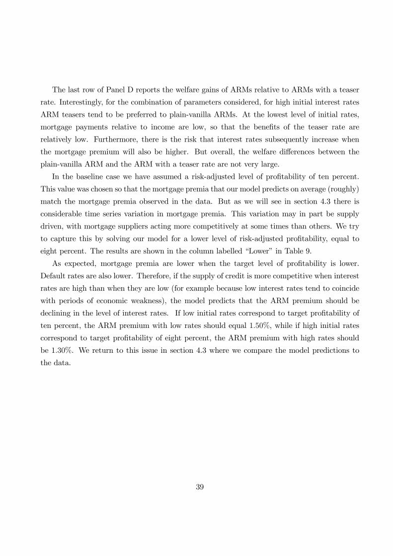
The last row of Panel D reports the welfare gains of ARMs relative to ARMs with a teaser
rate. Interestingly, for the combination of parameters considered, for high initial interest rates
ARM teasers tend to be preferred to plain-vanilla ARMs. At the lowest level of initial rates,
mortgage payments relative to income are low, so that the bene�ts of the teaser rate are
relatively low. Furthermore, there is the risk that interest rates subsequently increase when
the mortgage premium will also be higher. But overall, the welfare di¤erences between the
plain-vanilla ARM and the ARM with a teaser rate are not very large.
In the baseline case we have assumed a risk-adjusted level of pro�tability of ten percent.
This value was chosen so that the mortgage premia that our model predicts on average (roughly)
match the mortgage premia observed in the data. But as we will see in section 4.3 there is
considerable time series variation in mortgage premia. This variation may in part be supply
driven, with mortgage suppliers acting more competitively at some times than others. We try
to capture this by solving our model for a lower level of risk-adjusted pro�tability, equal to
eight percent. The results are shown in the column labelled �Lower�in Table 9.
As expected, mortgage premia are lower when the target level of pro�tability is lower.
Default rates are also lower. Therefore, if the supply of credit is more competitive when interest
rates are high than when they are low (for example because low interest rates tend to coincide
with periods of economic weakness), the model predicts that the ARM premium should be
declining in the level of interest rates. If low initial rates correspond to target pro�tability of
ten percent, the ARM premium with low rates should equal 1:50%, while if high initial rates
correspond to target pro�tability of eight percent, the ARM premium with high rates should
be 1:30%. We return to this issue in section 4.3 where we compare the model predictions to
the data.
39

4 Conditional Default Rates
In the previous section we have, for each level of initial interest rates, characterized the mortgage
premia, default, cash-out and re�nancing rates predicted by our model, calculated as average
rates across the eight hundred di¤erent paths for the aggregate variables that we have generated
(and across the realizations for the individual labor income shocks). Of course, ex post only
one of the paths for the aggregate variables will be realized, and the realized default rates may
be higher or lower than those reported.
We now focus on the conditional default probabilities predicted by our model, or on how
default probabilities di¤er across the di¤erent paths for the aggregate variables. From a poli-
cymaker�s point of view, the concern is those states with a large incidence of mortgage default.
This analysis also allows us to study the relative contribution of aggregate and idiosyncratic
shocks to the default decision. In section 4.1 we study di¤erences in default rates across ag-
gregate states, focusing on those states in which there is a high incidence of mortgage defaults.
In section 4.2 we study default rates for a path for the aggregate variables that resembles the
recent U.S. experience, with low interest rates and declining house prices. This is the path
that is more useful for understanding the �nancial crisis. In section 4.3 we compare the model
predictions to the data.
4.1 Di¤erences in default across aggregate states
Recall that in our model the aggregate shocks are shocks to real house prices, the in�ation rate,
and the real interest rate. The past realizations of house price and in�ation shocks determine
the current level of real house prices and the current price level, respectively. When we refer
to an aggregate state, we mean one possible combination of these aggregate shocks, out of the
eight hundred that we have generated.
In order to characterize the di¤erences in default rates across aggregate states, in Figure 3
we plot the proportion of aggregate states with given default frequencies. Panel A conditions
on a low initial interest rate, and Panel B on a high initial interest rate. Results are shown
both for the baseline level and for a higher level of labor income risk. The red bars in the
�gure show the proportion of aggregate states with any defaults at all (in practice, these are
states where house prices fall below the initial level for some period of time). The grey dashed
40

bars show the expected default rate, conditional on any defaults occurring in a state, and the
blue bars (plotted on a di¤erent vertical scale shown on the right axis of the �gure) show the
proportion of aggregate states with an extreme default wave, de�ned as defaults by at least
80% of outstanding mortgages.
The comparison of Panels A and B, which di¤er in initial rates, shows that both expected
default rates and the probability of a default wave are higher for ARMs when initial rates are
low, but higher for FRMs when initial rates are high. The �rst result is due to the fact that
interest rate increases, combined with house price declines, can trigger ARM default waves. The
second result is due to the fact that high initial rates imply large FRM premia. If house prices
and interest rates subsequently decline, many FRM borrowers who cannot re�nance their loans
decide to default. Higher labor income risk increases the number of states in which borrowers
�nd it optimal to default, but the e¤ects are much more pronounced when initial rates are high
than when they are low.
In order to further characterize the di¤erent aggregate states, in Figure 4 we plot the average
evolution of nominal house prices and interest rates for states with extreme default waves.
We plot such averages for both ARMs and FRMs and for two di¤erent levels of initial rates
(in panel A and panel B respectively), up to age 45 since no default occurs after this age.
Unsurprisingly, for both ARMs and FRMs, default waves tend to occur in aggregate states
with large house prices declines, of roughly �fty percent on average. Default waves occur 5-10
years after mortgage initiation, because it takes time for house prices to decline this far. In
addition, for low initial yields, default waves for ARMs tend to occur at higher levels of interest
rates than for FRMs. On the other hand, for high initial yields, a larger decline in interest rates
triggers FRM default. However, the di¤erences between ARM and FRM interest rates are not
very large, re�ecting the fact that in states of large house price declines, house prices and the
level of negative equity become the most important determinant of the default decision.
4.2 Recent US experience
One path for the aggregate variables that is particularly interesting to analyze is one that
matches the recent U.S. experience, characterized by declining house values after 2006 and low
interest rates after 2007 and particularly after 2008. With this in mind we set the aggregate
41
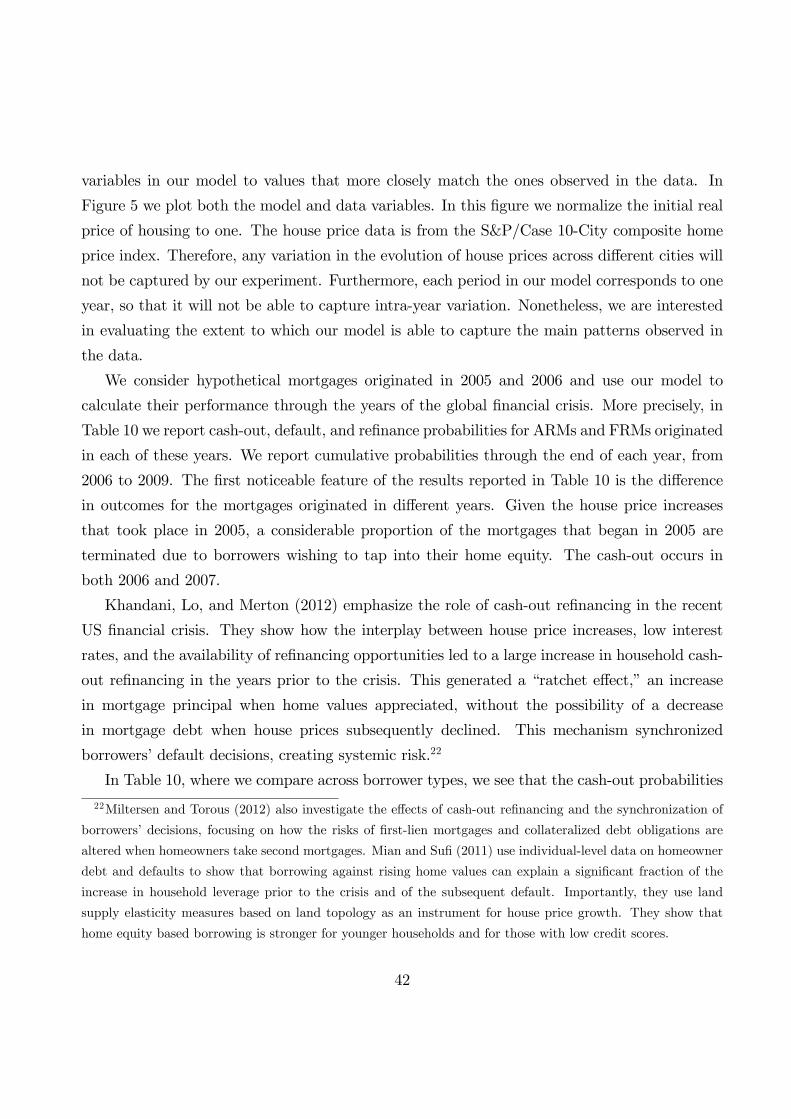
variables in our model to values that more closely match the ones observed in the data. In
Figure 5 we plot both the model and data variables. In this �gure we normalize the initial real
price of housing to one. The house price data is from the S&P/Case 10-City composite home
price index. Therefore, any variation in the evolution of house prices across di¤erent cities will
not be captured by our experiment. Furthermore, each period in our model corresponds to one
year, so that it will not be able to capture intra-year variation. Nonetheless, we are interested
in evaluating the extent to which our model is able to capture the main patterns observed in
the data.
We consider hypothetical mortgages originated in 2005 and 2006 and use our model to
calculate their performance through the years of the global �nancial crisis. More precisely, in
Table 10 we report cash-out, default, and re�nance probabilities for ARMs and FRMs originated
in each of these years. We report cumulative probabilities through the end of each year, from
2006 to 2009. The �rst noticeable feature of the results reported in Table 10 is the di¤erence
in outcomes for the mortgages originated in di¤erent years. Given the house price increases
that took place in 2005, a considerable proportion of the mortgages that began in 2005 are
terminated due to borrowers wishing to tap into their home equity. The cash-out occurs in
both 2006 and 2007.
Khandani, Lo, and Merton (2012) emphasize the role of cash-out re�nancing in the recent
US �nancial crisis. They show how the interplay between house price increases, low interest
rates, and the availability of re�nancing opportunities led to a large increase in household cash-
out re�nancing in the years prior to the crisis. This generated a �ratchet e¤ect,�an increase
in mortgage principal when home values appreciated, without the possibility of a decrease
in mortgage debt when house prices subsequently declined. This mechanism synchronized
borrowers�default decisions, creating systemic risk.22
In Table 10, where we compare across borrower types, we see that the cash-out probabilities
22Miltersen and Torous (2012) also investigate the e¤ects of cash-out re�nancing and the synchronization of
borrowers�decisions, focusing on how the risks of �rst-lien mortgages and collateralized debt obligations are
altered when homeowners take second mortgages. Mian and Su� (2011) use individual-level data on homeowner
debt and defaults to show that borrowing against rising home values can explain a signi�cant fraction of the
increase in household leverage prior to the crisis and of the subsequent default. Importantly, they use land
supply elasticity measures based on land topology as an instrument for house price growth. They show that
home equity based borrowing is stronger for younger households and for those with low credit scores.
42

predicted by our model tend to be larger for borrowers who face large income risk, particularly
so when the level of income is correlated with interest rates. For these borrowers, the fall in
interest rates and incomes in 2007 leads them to tap into their home equity. One way to think
of these borrowers who tap into home equity is that they take out a new mortgage in a later
year with a higher loan-to-value than their existing mortgage. Our model predicts that riskier
borrowers were more likely to do so, and it suggests that in the years leading up to the �nancial
crisis the pool of new borrowers in the market may have had an increasing proportion of riskier
borrowers. Furthermore, recall that our model predicts that borrowers who face large income
risk are more likely to prefer ARMs, so that the pool of ARM borrowers may have become
increasingly risky.
Table 10 also shows that in 2007, as interest rates decline, many FRMs initially taken out in
2005 are re�nanced. After this year, we start seeing some default. Default rates are on average
higher for ARMs than FRMs, with the exception of the case of high income risk correlated
with interest rates. However, recall that the model predicts that borrowers with this type of
income risk are the ones who would bene�t the most from ARMs relative to FRMs (Table 7), so
that the results for the FRM with correlated income risk should be seen as a hypothetical case
whose results are shown for comparison, but that we would not expect to observe in reality.
The �nal column of Table 10 reports results for the mortgages originated in 2006, just before
house prices started to decline. Given the immediate decline in house prices we do not observe
any cash-out for these mortgages. Furthermore, negative home equity prevents FRM borrowers
from re�nancing their mortgages. We observe some default as early as 2006, but it only becomes
more prevalent in later years, as house prices decline further and borrowers �nd themselves with
more negative home equity. Among the di¤erent borrower types considered, default rates tend
to be larger for borrowers with higher income risk, and income that is correlated with interest
rates. Again, the model predicts that these borrowers are the ones who, when taking out a
mortgage in 2006, would bene�t the most from an ARM relative to the FRM.
In the next section we compare these model predictions to data. Before we do so, we note
that in the several experiments we have reported in Table 10, the initial LTI and LTV are
equal to the baseline values of 4.5 and 0.90, respectively. The corresponding real house value is
$231.8 thousand. In 2005, given that we have normalized real house prices to one, this is also
house size. However, in 2006 real house prices are higher than in 2005, and equal to 1.16. For
43

same house value, it has to be case that borrowers in 2006 are buying houses of a smaller size,
equal in size to a house of value 231:8=1:16 = 198:9 thousand in 2005. In this case, since we
have assumed separability between housing and non-durable consumption, and that house size
is �xed throughout, our calculations go through. An alternative approach would have been to
assume that individuals are buying the same size house in 2006 as in 2005, that they use the
same dollar amount for the downpayment, but that they need to take out a loan with a higher
initial loan-to-value and a higher multiple of labor income.
4.3 Empirical evidence
There are at least four di¤erent dimensions along which we can evaluate the extent to which
our model is able to capture the patterns observed in the data: mortgage premia, mortgage
choice, re�nancing patterns, and default rates. We discuss these in turn. For the �rst two we
use data from the Monthly Interest Rate Survey of the Federal Housing Finance Agency. We
use information on the e¤ective rates for ARMs and FRMs, on their LTV, on the loan amount,
and also on the proportion of new mortgages that are of the FRM type (the FRM share). To
calculate mortgage premia we use the yields on zero-coupon bonds from Gurkaynak, Sack, and
Wright (2006). We calculate the premium for ARMs as the di¤erence relative to the yield on
1-year zero coupon bonds and the premium for FRMs as the di¤erence relative to the yield on
a 20-year annuity (consistent with our model analysis in the previous section). We also use CPI
data from the Bureau of Labor Statistics to calculate real loan amounts.
4.3.1 Mortgage premia and choice
Figure 6, Panel A plots the history of mortgage premia on ARMs and of one-year bond yields.
Panel B shows a corresponding plot for FRMs, adding the slope of the term structure of Treasury
yields. Both �gures cover the sample period for which data is available, 1986:01 to 2008:10. It
is immediately apparent from the �gure that the ARM premium is much more volatile than the
FRM premium, and there is a strong tendency for the ARM premium to decline with the level
of interest rates. On the other hand the FRM premium seems to increase modestly with the
level of interest rates. In order to facilitate comparison with the model, in Panel A of Table 11
we report the average mortgage premia that we observe in the data. We do so in two di¤erent
44

ways. In Panel A.1, we match the observations in the data to those in the model based on the
level of 1-year bond yields, which is reported in the �rst line of the panel, and then calculate
the average premia. In Panel A.2, we repeat the same exercise based on the slope of the term
structure of interest rates. The di¤erences between the two are mainly due to the fact that
in our model, for the highest level of interest rates, the slope of the term structure is steeply
negative, which has not happened in the data during the sample period.
For comparison, in panel B we report the mortgage premia predicted by our model. In
Panel B.1 we report results for ARMs and in Panel B.2 for FRMs. Recall that in our model
short rates do not vary independently from the slope of the term structure. Focusing �rst on
FRMs, we see that generally our model predicts mortgage premia that increase more steeply
with the level of interest rates than the increase that we observe in the data. This is due to
the re�nancing option being increasingly valuable as interest rates increase. The model with
re�nancing inertia predicts an increase in FRM mortgage premia that is more in line with that
observed in the data. In addition our model seems to do a reasonable good job at matching
FRM mortgage premia for LTI equal to 4.5 and a lower LTV equal to 0.80, when we match it
to the data using the slope of the term structure. Alternatively, if the pool of FRM borrowers
becomes safer when interest rates increase, or if target pro�tability is lower when interest rates
are high, then this will contribute to relatively lower FRM premia when interest rates are high.
The di¤erences between the model and the data are much more pronounced for ARM
mortgage premia. In the data there is signi�cantly more variation than in the model, and
contrary to the model base case, ARM premia in the data decrease signi�cantly with the
level of short rates and the slope of the term structure. Of all the model cases that we have
considered, the only one that delivers such a decreasing pattern is the case in which borrowers
face a higher income risk that is positively correlated with the short-term interest rate. This
case is particularly interesting because for such borrowers ARMs provide large hedging bene�ts,
which makes it much more likely that they choose to borrow in this form. But the table shows
that even in this case, the decrease in mortgage premia that the model predicts is smaller than
the one observed in the data.
The much higher mortgage premia for ARMs when interest rates are low may potentially
be explained by selection of riskier borrowers into ARMs when interest rates are low. If such
selection occurs, and mortgage lenders are aware of this phenomenon, they may increase ARM
45

premia to compensate during periods of low interest rates. The FHFA data does not have
information on borrower characteristics, but it does tell us LTV ratios, and Table 12 reports
regression results of mortgage premia on bond yields and LTV. As Figure 6 already showed,
the mortgage premium for ARMs is higher when short-term yields are low. It is also higher
when the LTV on ARMs is large relative to the LTV on FRMs, consistent with the notion that
riskier borrower composition increases the mortgage premium.
However, the mortgage premium for ARMs is negatively related to the LTV for ARMs.
Similarly, the mortgage premium for FRMs is negatively related to the LTV for FRMs. One
plausible explanation is that easing credit conditions both reduce credit spreads and increase
LTV. A possible (if fairly crude) way to think about easing credit conditions in the context of
our model is to assume that at such times there is increased competition among lenders which
leads to a lower level of target pro�tability. If that happens when interest rates are high, then
this may at least partially explain the reduction in premia that we observe in the data for high
interest rates.
Although our model is partially successful at generating the qualitative patterns of mortgage
premia that we observe in the data, the quantitative variation in mortgage premia for ARMs is
much larger in the data than in any of our model-based experiments. To achieve larger variation
in mortgage premia we would need to consider more extreme cases than those considered.
Figure 7 plots the evolution over time of the ARM share, illustrating the fact that the
popularity of ARMs is positively correlated with the 1-year yield. The correlation between the
two series is equal to 0:56. As in the data, the model predicts that borrowers are more likely
to prefer an ARM when interest rates are high and a FRM when interest rates are low. But
Figure 7 also shows that in the data there is variation in the ARM share that is independent
of the short rate. This may in part re�ect changes in the composition of borrowers.
4.3.2 Mortgage re�nancing and default
To measure re�nancing activity, we use quarterly data from the Freddie Mac Cash-Out Re�-
nance report. In Panel A of Figure 8 we plot the proportion of re�nances that result in a 5%
or greater increase in loan amount, alongside information on 1-year bond yields. The �gure
shows that the proportion of re�nances that involve signi�cant cash-out is strongly positively
correlated with the level of interest rates. The correlation between the two series is as high
46

as 0.80. Or in other words, and unsurprisingly, interest-rate re�nancing tends to occur when
interest rates are low. In Panel B we plot the total quantity of home equity cashed out and the
annual change in the Case-Shiller 10 City Composite U.S. house price index. In this �gure we
see that the large increases in house prices in the early to mid 2000s were followed by signi�cant
amounts of cashing out, particularly in the period from 2005 through early 2007, even at a time
when house prices were already starting to drop. These patterns are broadly consistent with
what our model predicts in the di¤erent experiments that we have carried out in Table 10.
Figure 9 plots quarterly foreclosures initiated by loan type, using data from the National
Delinquency Survey. An intriguing feature of the data clearly visible in the �gure is that in
spite of the low interest rate environment that followed the onset of the crisis, default rates for
ARMs were considerably higher than for FRMs, both among prime and subprime borrowers.
Figure 9 also shows that some foreclosures were initiated in 2006 and early 2007, but the
number of initiations greatly increased in 2008 and 2009. Our model is consistent with both
these features of the data. Table 10 shows that our model is able to generate default rates
higher for ARMs than for FRMs if those borrowers who took out ARMs have higher labor
income risk. Importantly, we also �nd that these same borrowers tend to bene�t more from
ARMs ex ante, that is, at the time the mortgage was chosen. Table 10 also shows some default
occurring in 2006, but much higher defaults in later years.
5 Conclusion
We have proposed a rational life-cycle model of household behavior, incorporating risks to labor
income, house prices, in�ation, and interest rates, to understand the types of mortgages that
borrowers take out and their subsequent decisions to re�nance, cash out, or default on those
mortgages. In our model, competitive lenders set mortgage rates to achieve a target level
of risk-adjusted pro�tability, and the model takes into account the two-way feedback between
mortgage rates and borrower decisions.
Our model highlights the fact that default depends not only on the extent to which a
borrower has negative home equity, but also on the extent to which borrowers are constrained
by low current resources. These two factors are sometimes described by mortgage practitioners
as �dual triggers�of default. In our model, constraints shift the threshold at which a borrower
47

optimally decides to exercise the irreversible option to default.
We use our model to explore several policy issues concerning mortgages. The relative
merits of adjustable-rate mortgages (ARMs) and �xed-rate mortgages (FRMs) have been much
debated, with some commentators arguing that ARMs are inherently more prone to default, a
position that seems to be supported by high ARM default rates during the recent US housing
downturn. In our model, ARMs and FRMs have similar overall default rates, and similar
sensitivities to the level of house prices, but the other drivers of default are di¤erent. ARM
defaults tend to occur when interest rates and in�ation increase, driving up required payments
on ARMs, while FRM defaults tend to occur when interest rates and in�ation decrease. For this
reason ARM default risk is highest for mortgages originated at low rates, while FRM default
risk is highest for mortgages originated at high rates.
This raises the question why ARM defaults were so high in the US housing downturn,
even while interest rates were declining. We argue that one plausible explanation is selection
of borrowers with riskier income, and income positively correlated with interest rates, into
ARMs. In our model such borrowers favor ARMs, particularly when interest rates are initially
low. Another contributory factor may have been the modi�cation of plain-vanilla ARMs to
incorporate teaser rates and other devices to defer mortgage repayment. Unsurprisingly we
show that such deferral of principal repayment tends to increase default rates.
Our model also has implications for the pattern of mortgage premia as interest rates vary.
The model implies that FRM premia tend to increase with the initial level of interest rates,
because high initial interest rates increase the value of the borrower�s options to re�nance, or
to default if re�nancing is prevented by declines in house prices. This increase in FRM premia
makes FRMs relatively less attractive to borrowers when interest rates are high, consistent with
US experience during the early 1980s. With a constant composition of borrowers, our model
implies that ARM premia are slightly increasing with the initial level of interest rates. However
this pattern can be reversed, thereby improving the �t to historical US data, by selection of
riskier borrowers into ARMs when initial rates are low. Our baseline model with fully rational
households generates excessively strong responses of mortgage premia to interest rates, but
these responses are moderated if households re�nance more slowly than is optimal.
Although our model has a rich stochastic structure that includes many realistic aspects of
mortgage markets, the need to economize on state variables has prevented us from capturing
48

certain phenomena that we leave for future research. In the paper we assume an exogenously
�xed house size, and present only limited results for a model of endogenous housing choice in
the online appendix. In the paper we assume that mortgage lenders have no recourse in the
event of default, an assumption that is accurate for some US states but not for others, and
we present only limited results for recourse mortgages in the online appendix. We allow a
limited form of cash-out re�nancing, modeled as selling a house to tap positive home equity
and moving to rental accommodation, but we do not study second mortgages or home equity
lines of credit. Our model does not include unsecured borrowing or bankruptcy, and it does
not allow households to invest in risky assets such as long-term bonds or equities.
Beyond addressing these limitations of the current model, there are several other interesting
directions for future research. First, we can use microeconomic data on mortgage choice,
mortgage premia, delinquency, and default to structurally estimate our model parameters and
to test the predictions of the model across households and mortgage types. Second, we can
assess the risk, systemic and otherwise, of portfolios of mortgages. Of particular interest is the
di¤erential response of FRM and ARM default to interest-rate movements. This is relevant for
monetary authorities in areas such as the eurozone in which these types of mortgages co-exist.
Third, we can study the e¤ects of structural changes in mortgage markets such as declining
underwriting standards (which could be captured by lower pro�tability targets for mortgage
lenders) or changes in implicit subsidies from government mortgage credit guarantees. We can
also study mortgage features that are standard in other countries but not in the US, such as
the ability of FRM borrowers in Denmark to re�nance (without increasing mortgage principal)
even when they have negative home equity. Finally, we can use our model to analyze mortgage
modi�cation policies that are intended to reduce the incidence of default in the aftermath of
severe declines in house prices.
49

6 References
Amromin, Gene, Jennifer Huang, Clemens Sialm, and Edward Zhong, 2011, �Complex Mort-
gages,�NBER Working Paper No. 17315.
Bajari, Patrick, Chenghuan Sean Chu, and Minjung Park, 2008, �An Empirical Model of
Subprime Mortgage Default From 2000 to 2007,�NBER Working Paper No. 14625.
Bhutta, Neil, Jane Dokko, and Hui Shan, 2010, �The Depth of Negative Equity and Mort-
gage Default Decisions,�Finance and Economics Discussion Series No. 2010-35, Federal
Reserve Board.
Brueckner, Jan K., 1994, �Borrower Mobility, Adverse Selection, andMortgage Points,�Journal
of Financial Intermediation, 3, 416-441.
Campbell, John Y., 2006, �Household Finance,�Journal of Finance, 61, 1553�1604.
Campbell, John Y. and Joao F. Cocco, 2003, �Household Risk Management and Optimal
Mortgage Choice,�Quarterly Journal of Economics, 118, 1449�1494.
Campbell, John Y. and Joao F. Cocco, 2014, �A Model of Mortgage Default: Appendix�,
available online at authors�websites.
Campbell, John Y., Stefano Giglio, and Parag Pathak, 2011, �Forced Sales and House Prices�,
American Economic Review 101, 2108�2131.
Campbell, Sean D., Morris A. Davis, Joshua Gallin, and Robert M. Martin, 2009, �What
Moves Housing Markets: A Variance Decomposition of the Rent-Price Ratio,�Journal of
Urban Economics, 66, 90�102.
Campbell, Tim S., and J. Kimball Dietrich, 1983, �The Determinants of Default on Insured
Conventional Residential Mortgage Loans,�The Journal of Finance, 37, 5.
Carroll, Christopher D., 1997, �Bu¤er-Stock Saving and the Life-Cycle/Permanent Income
Hypothesis,�Quarterly Journal of Economics 114, 433�495.
50

Carroll, Christopher D. and Andrew Samwick, 1997, �The Nature of Precautionary Wealth,�
Journal of Monetary Economics, 40(1).
Chan, Sewin, 2001, �Spatial Lock-in: Do Falling House Prices Constrain Residential Mobility,�
Journal of Urban Economics 49, 567�586.
Chatterjee, Satyajit, and Burcu Eyigungor, 2009, �Foreclosures and House Price Dynamics:
A Quantitative Analysis of the Mortgage Crisis and The Foreclosure Prevention Policy,�
Working Paper, Federal Reserve Bank of Philadelphia.
Chen, Hui, Michael Michaux and Nikolai Roussanov, 2013, �Houses as ATMs? Mortgage
Re�nancing and Macroeconomic Uncertainty,�Working Paper, MIT Sloan, USC and
Wharton.
Cocco, Joao F., 2013, �Evidence on the Bene�ts of Alternative Mortgage Products,�Journal
of Finance, 68, 1663�1690.
Corbae, Dean, and Erwan Quintin, 2013, �Leverage and the Foreclosure Crisis,�Working
Paper, University of Wisconsin.
Corradin, Stefano, 2012, �Household Leverage,�ECB Working Paper 1452, European Central
Bank.
Curcuru, Stephanie, John Heaton, Deborah Lucas, and Damien Moore, 2010, �Heterogeneity
and Portfolio Choice: Theory and Evidence,�The Handbook of Financial Econometrics,
volume 1, 337�382.
Das, Sanjiv R., 2011, �The Principal Principle: Optimal Modi�cation of Distressed Home
Loans,�Working Paper, Santa Clara University.
Deaton, Angus S., 1991, �Savings and Liquidity Constraints,�Econometrica 59, 1221�1248.
Demyanyk, Yuliya, Ralph S.J. Koijen, and Otto Vam Hemert, 2010, �Determinants and Con-
sequences of Mortgage Default,�Working Paper, Fedreal Reserve Bank of Cleveland and
University of Chicago.
51

Deng, Yongheng, John M. Quigley, and Robert Van Order, 2000, �Mortgage Terminations,
Heterogeneity and the Exercise of Mortgage Options,�Econometrica, Vol. 68, No. 2,
275-307.
Diaz, Antonia and Maria-Jose Luengo-Prado, 2008, �On the User Cost and Homeownership,�
Review of Economic Dynamics 11, 584�613.
Doviak, Erik, and SeanMacDonald, 2009, �Who Defaults? Who goes into Foreclosure?,�Working
paper, City University of New York.
Elul, Ronen, Nicholas Souleles, Souphala Chomsisengphet, Dennis Glennon, and Robert Hunt,
2010,�What �Triggers�Mortgage Default?,� American Economic Review Papers and Pro-
ceedings, 100, 490 �494.
Financial Services Authority, 2009, �Mortgage Market Review,�Discussion Paper 09/3.
Foote, Christopher, Kristopher Gerardi, and Paul Willen, 2008, �Negative Equity and Fore-
closure: Theory and Evidence,�Journal of Urban Economics, 6 (2), 234 �245.
Foote, Christopher, Kristopher Gerardi, Lorenz Goette, and Paul Willen, 2010, �Reducing
Foreclosures: No Easy Answers�, in NBER Macroeconomics Annual 2009, University of
Chicago Press, 89�138.
Friedman, Milton, 1957, A Theory of the Consumption Function, Princeton University Press.
Garriga, Carlos, and Don E. Schlagenhauf, 2009, �Home Equity, Foreclosures, and Bail-outs,�
Working paper, Federal Reserve Bank of St. Louis and Florida State University.
Gerardi, Kristopher, Harvey S. Rosen and Paul Willen, 2010, �The Impact of Deregulation
and Financial Innovation on Consumers: The Case of The Mortgage Market,�Journal of
Finance 65, 333�360.
Ghent, A. and M. Kudlyak, 2011, �Recourse and Residential Mortgage Default: Evidence
from U.S. States,�Review of Financial Studies 24, 3139�3186.
Ghent, A., 2011, �Subprime Mortgages, Mortgage Choice, and Hyperbolic Discounting,�
Working Paper, Zicklin School of Business.
52

Glaeser, Edward L. and Jesse M. Shapiro, 2003, �The Bene�ts of the Home Mortgage Interest
Deduction,�Tax Policy and the Economy, 17.
Gourinchas, Pierre-Olivier and Jonathan Parker, 2002, �Consumption Over The Life Cycle,�
Econometrica 70, 47�89.
Guiso, Luigi, Paola Sapienza and Luigi Zingales, 2013, �The Determinants of Attitudes To-
wards Strategic Default on Mortgages,�Journal of Finance 68, 1473�1515.
Guiso, Luigi, and Paolo Sodini, 2013, �Household Finance: An Emerging Field,� in George
Constantinides, Milton Harris, and Rene Stulz eds., Handbook of the Economics of Fi-
nance, Volume 2B, North-Holland, 1397�1531.
Gurkaynak, Refet, Brian Sack, and Jonathan H. Wright, 2006, �The U.S. Treasury Yield
Curve: 1961 to the Present,�Finance and Economics Discussion Series, Federal Reserve
Board.
Haughwout, Andrew, Ebiere Okah and Joseph Tracy, 2010, �Second Chances: Subprime Mort-
gage Modi�cation and Re-Default,�Working Paper, Federal Reserve Bank of New York.
Himmelberg, Charles, Christopher Mayer and Todd Sinai, 2005, �Assessing High House Prices:
Bubbles, Fundamentals and Misperceptions,�Journal of Economic Perspectives, 19, 67-
92.
Khandani, Amir E., Andrew W. Lo, and Robert C. Merton, 2012, �Systemic Risk and the
Re�nancing Ratchet E¤ect,�Working Paper, MIT.
Koijen, Ralph S.J. Otto Van Hemert, and Stijn Van Nieuwerburgh, 2009, �Mortgage Timing,�
Journal of Financial Economics, 93, 292-324.
Krainer, John, Stephen Leroy, and O Munpyung, 2009, �Mortgage Default and Mortgage
Valuation,�Working Paper, Federal Reserve Bank of San Francisco and University of
California Santa Barbara.
Li, Wenli, Michelle J. White, and Ning Zhu, 2010, �Did Bankruptcy Reform Cause Mortgage
Default to Rise?,�NBER Working Paper, 15968.
53

Lusardi, Annamaria and Olivia Mitchell, 2007, �Baby Boomer Retirement Security: The Roles
of Planning, Financial Literacy, and Housing Wealth,�Journal of Monetary Economics,
54, 205-224.
Mayer, Christopher, Karen Pence and Shane Sherlund, 2009, �The Rise in Mortgage Defaults,�
Journal of Economic Perspectives, 23, Number 1, 27-50.
Mian, Atif and Amir Su�, 2009, �The Consequences of Mortgage Credit Expansion: Evidence
from the U.S. Mortgage Default Crisis,�Quarterly Journal of Economics, 124, 4.
Mian, Atif and Amir Su�, 2011, �House Prices, Home Equity-Based Borrowing, and the U.S.
Household Leverage Crisis,�American Economic Review, 101, 5.
Miles, David, 2004, The UK Mortgage Market: Taking a Longer-term View, HM Treasury.
Miltersen, Kristian R. and Walter N. Torous, 2012, �Second Mortgages: Valuation and Impli-
cations for the Performance of Structured Financial Products,�Working Paper, Copen-
hagen Business School and MIT.
Mitman, Kurt, 2012, �The Macroeconomic E¤ects of Bankruptcy and Foreclosure Policies,�
Working Paper, Penn Institute For Economic Research.
Narita, Machiko, 2011, �Understanding the Housing Bust: Disentangling Credit Crunch and
Severe Recession,�Working Paper, University of Minnesota and Federal Reserve Bank of
Minneapolis.
Piazzesi, Monika, Martin Schneider and Selale Tuzel, 2007, �Housing, Consumption, and Asset
Pricing,�Journal of Financial Economics, 83, 531-569.
Piazzesi, Monika, and Martin Schneider, 2010, �In�ation and the Price of Real Assets,�Work-
ing Paper, Stanford University.
Piskorski, Tomasz and Alexei Tchistyi, 2010, �Optimal Mortgage Design,�Review of Financial
Studies 23, 3098�3140.
Piskorski, Tomasz and Alexei Tchistyi, 2011, �Stochastic House Appreciation and Optimal
Subprime Lending,�Review of Financial Studies 24, 1407�1446.
54

Poterba, James M., 1984, �Tax Subsidies to Owner-Occupied Housing: An Asset-Market
Approach,�The Quarterly Journal of Economics, 99, 729�752.
Poterba, James M., and Todd Sinai 2011, �Revenue Costs and Incentive E¤ects of Mortgage
Interest Deduction For Owner-Occupied Housing,�The National Tax Journal, 64, 531�
564.
Schwartz, Eduardo S. and Walter N. Torous, 2003, �Mortgage Prepayment and Default Deci-
sions: A Poisson Regression Approach,�Real Estate Economics, 21, 4, 431-449.
Sinai, Todd and Nicholas Souleles, 2005, �Owner-Occupied Housing as a Hedge Against Rent
Risk,�Quarterly Journal of Economics, 120, 2, 763-789.
Stanton, Richard and Nancy Wallace, 1998, �Mortgage Choice: What�s the Point?,� Real
Estate Economics, 26, 173-205.
Stanton, Richard and Nancy Wallace, 1999, �Anatomy of an ARM: The Interest Rate-Risk
of Adjustable-Rate Mortgages,�Journal of Real Estate and Finance and Economics, 19,
49-67.
Vandell, Kerry D., 1978, �Default Risk Under Alternative Mortgage Instruments,�The Journal
of Finance, 33, 5, 1279-1296.
Zeldes, Stephen, 1989, �Optimal Consumption with Stochastic Income: Deviations from Cer-
tainty Equivalence�, Quarterly Journal of Economics 104, 275�298.
55

Figure 1: Loan-to-value, mortgage payment-to-income and loan-to-income over time for the US.
10
20
30
40
50
60
70
80
90
84 85 86 87 88 89 90 91 92 93 94 95 96 97 98 99 00 01 02 03 04 05 06 07 08
Year
Loan
-to-
valu
e an
d M
ortg
age
Pay
men
t-to
-In
com
e (
per
cent
)
2.5
3
3.5
4
4.5
5
Loan
-to-
Inco
me
Loan-to-value Mortgage payment-to-income Loan-to-income
Note to Figure 1: The LTV data are from the Monthly Interest Rate Survey (MIRS), the LTI data are calculated as the ratio of the average loan amount obtained from the same survey to the median US household income obtained from Census data, the mortgage payment to income are calculated using the same income measure and the loan amount, maturity and mortgage interest rate data from the MIRS.

Figure 2: Difference in mortgage payments to household income between households who default and who do not default and proportion of defaults as a function of home equity for the ARM contract.
Panel A.1: Low initial yield, low income risk Panel A.2: High initial yield, low income risk
Panel B.1: Low initial yield, high income risk Panel B.2: High initial yield, high income risk
Note to Figure 2: The data are generated from simulating the model for the ARM contract. Low (high) income risk refers households with a standard deviation of temporary income shocks equal to 0.225 (0.35). Loan to value is the ratio of current house value to the outstanding loan principal. The vertical bars plot, for each level of negative home equity, Mortgage Payments/Income for those households who choose to default minus Mortgage Payments/Income for those households who choose not to default.

Figure 3: Proportion of aggregate states with a given default frequencies.
Panel A: Low initial yield
Panel B: High initial yield
Note to Figure 3: This figure reports the proportion of aggregate states with a positive mortgage default and with a default rate higher than 80%, by initial yield and mortgage type for different levels of income risk. Low (high) income risk refers households with a standard deviation of temporary income shocks equal to 0.225 (0.35). In addition the figure reports the average default rate across states with positive default. The data are obtained by simulating the model with the parameters shown in Table 1.

Figure 4: Aggregate characteristics of default waves.
Panel A: Low initial yield
Panel B: High initial yield
Note to Figure 4: This figure plots nominal house prices, nominal interest rates, and proportion of defaults for aggregate states with a default rate over 80% by mortgage type. Low (high) initial yield refers to the initial interest rates. The data are obtained by simulating the model with the parameters shown in Table 1. The figure plots the data until age 45 since no default occurs after this age.

Figure 5: Real house prices and nominal interest rates in the model and in the data.
Note to Figure 5: This figure plots real house prices and nominal interest rates over time in the data and in the model. The house price data is the Case-Shiller US 10-cities composite index and the interest rate data is from the Federal Reserve. House prices in 2005 are normalized to one.

Figure 6: Evolution of mortgage premia over time in the data
Panel A: ARMs
Panel B: FRMs
Note to Figure 6: This figure plots the evolution over time of mortgage premia, one-year zero-coupon bond yields, the slope of the term structure, and of mortgage premia. Mortgage premia for ARMs are calculated as the difference between the effective ARM rate and the yield on 1-year zero coupon bonds. Mortgage premia for FRMs are calculated as the difference between the effective FRM rate and the yield on a 20-year annuity. The mortgage data are from the Monthly Interest Rate Survey of the Federal Housing Finance Agency. The data on yields are from the Federal Reserve Board.

Figure 7: Evolution of the ARM share of new mortgages over time in the data
Note to Figure 7: This figure plots the evolution over time of the proportion of new mortgages that are of the ARM type. The figure also plots the one-year zero-coupon bond yields, and the difference between the effective rate on ARMs and on FRMs. The mortgage data are from the Monthly Interest Rate Survey of the Federal Housing Finance Agency. The data on yields are from the Federal Reserve Board.

Figure 8: Refinancing activity
Panel A: Proportion of refinances resulting in a 5% or higher loan amount
Panel B: Cash-out amounts
Note to Figure 8: The refinancing data is from the Freddie Mac Cash-Out Refinance Report.

Figure 9: Foreclosures started by loan type (percent)
Note to Figure 9: The data are from the National Delinquency Survey of the Mortgage Bankers Association.

Table 1: Baseline parameters.
Description Parameter Value
Time and preference parameters
Discount factor 098
Risk aversion 2
Preference for housing 03
Initial age 20
Terminal age 50
Bequest motive 400
Inflation and real interest rate
Mean log inflation 0.029
Stdev of the inflation rate 0.009
Log inflation AR(1) coefficient 0.891
Mean log real rate 0.012
Stdev of the real rate 0.018
Log real rate AR(1) coefficient 0.825
Correl. inflation and real rate 0.597
Labor income and house prices
Mean log real income growth ∆ 0.008
Stdev permanent income shocks 0.063
Stdev temporary income shocks 0.225
Mean log real house price growth 0.003
Stdev house price return 0.162
Correl. perm. inc. and house price shocks 0.191
Correl. real int. rate and house price shocks 0.300
Correl. temp. inc. and inflation shocks 0.000
Tax rates and other parameters
Income tax rate 0.25
Property tax rate 0.015
Property maintenance 0.025
Lower bound on cash-on-hand $1,000
Transaction costs of house sale 0.060
Exogenous moving prob. 0.040
Exogenous mov. prob. if neg. equity 0 0.008
Loan Parameters
Initial loan to income 45
Initial loan to value 090
FRM refinancing cost 001
Note to Table 1: This table reports the parameter values used in the baseline case.

Table 2: Means for different variables for the ARM contract by household action, for different levels
of income risk, and conditional on initial interest rates.
A.1: Low initial rate, low income risk A.2: High initial rate, low income risk
Variable Def No def/Eq<0 Cash-out No act Def No def/Eq<0 Cash-out No act
Current ltv 1.43 1.11 0.42 0.55 1.41 1.15 0.43 0.54
Price level 1.17 1.08 1.29 1.26 1.23 1.17 1.35 1.32
Real house pr. 0.45 0.69 1.34 1.08 0.45 0.59 1.32 1.07
Real inc 46.6 47.7 48.8 52.5 46.3 48.0 48.5 52.6
Real cons t-1 13.9 15.1 13.4 14.9 13.4 14.2 12.9 14.5
Mort/Inc 0.33 0.29 0.31 0.28 0.33 0.33 0.33 0.30
(Mort-Rent)/Inc 0.26 0.22 0.05 0.12 0.26 0.24 0.05 0.11
Nom int rate 0.037 0.022 0.041 0.037 0.039 0.038 0.047 0.044
Age 36.4 33.2 39.3 38.3 36.4 34.6 39.0 38.3
Probability 0.044 0.583 0.037 0.595
B.1: Low initial rate, high income risk B.2: High initial rate high income risk
Variable Def No def/Eq<0 Cash-out No act Def No def/Eq<0 Cash-out No act
Current ltv 1.41 1.11 0.44 0.56 1.33 1.15 0.46 0.55
Price level 1.16 1.08 1.28 1.25 1.20 1.17 1.32 1.31
Real house pr. 0.46 0.69 1.32 1.07 0.51 0.59 1.29 1.07
Real inc 47.3 49.5 48.2 54.4 43.3 50.3 46.8 54.7
Real cons t-1 14.1 15.4 13.5 15.5 12.6 14.4 12.8 15.2
Mort/Inc 0.35 0.30 0.35 0.29 0.40 0.34 0.38 0.31
(Mort-Rent)/Inc 0.28 0.23 0.07 0.12 0.30 0.25 0.08 0.12
Nom int rate 0.037 0.022 0.041 0.036 0.040 0.038 0.047 0.044
Age 36.4 33.2 39.0 38.2 35.5 34.5 38.2 38.2
Probability 0.046 0.602 0.048 0.625
Note to Table 2: This table reports the mean for several variables for the ARM contract by household
action (default, no default given negative home equity, cash-out, no action). The table reports means
across aggregate states and individual shocks, conditional on the initial level of interest rates. Low
(High) initial rate corresponds to the state with the lowest (second highest) level of interest rates in our
model. The top (bottom) panels report results for the case in which the standard deviation of income
shocks is equal to 0.225 (0.35). For each case the first column reports means for observations in which
individuals choose to default, the second column reports means for observations in which individuals
have negative home equity but choose not to default, the third column reports means for observations
in which individuals choose to cash-out, and the last column reports means for observations in which
individuals choose neither to default nor to cash-out (in case they have not done so before). Current
loan-to-value is the loan to value at the time of the action (or the no action). In the means reported,
each observation corresponds to an individual and a time period. The probabilities of default and of
cash-out are the proportion of households who choose to default or to cash-out over the life of the
mortgage.

Table 3: Means for different variables for the FRM contract by household action, for different levels
of income risk, and conditional on initial interest rates.
A.1: Low initial rate, low income risk A.2: High initial rate, low income risk
Variable Def No def/Eq<0 Cash-out No act Def No def/Eq<0 Cash-out Ref No act
Current ltv 1.42 1.11 0.41 0.54 1.41 1.17 0.47 0.61 0.57
Price level 1.16 1.08 1.29 1.26 1.22 1.17 1.31 1.24 1.31
Real house pr. 0.47 0.68 1.34 1.08 0.46 0.59 1.38 0.98 1.15
Real inc 46.8 47.7 49.3 52.4 46.9 47.4 46.9 54.0 51.5
Real cons t-1 13.9 15.0 13.7 14.8 13.0 13.6 12.2 14.3 13.9
Mort/Inc 0.32 0.33 0.28 0.27 0.38 0.39 0.37 0.26 0.34
(Mort-Rent)/Inc 0.26 0.26 0.03 0.10 0.32 0.29 0.06 0.21 0.10
Nom int rate 0.027 0.023 0.040 0.037 0.031 0.042 0.050 0.008 0.053
Age 36.1 33.3 39.5 38.5 36.0 34.3 37.5 36.1 37.3
Probability 0.034 0.572 0.051 0.369 0.471
B.1: Low initial rate, high income risk B.2: High initial rate high income risk
Variable Def No def/Eq<0 Cash-out No act Def No def/Eq<0 Cash-out Ref No act
Current ltv 1.40 1.11 0.43 0.55 1.32 1.17 0.52 0.60 0.61
Price level 1.15 1.08 1.28 1.26 1.19 1.17 1.26 1.24 1.29
Real house pr. 0.48 0.68 1.32 1.07 0.52 0.60 1.31 1.01 1.12
Real inc 47.2 49.5 48.7 54.5 44.0 49.7 44.5 56.9 53.5
Real cons t-1 13.8 15.1 13.7 15.5 11.8 13.8 11.9 14.7 14.7
Mort/Inc 0.34 0.34 0.31 0.28 0.46 0.41 0.44 0.26 0.36
(Mort-Rent)/Inc 0.28 0.27 0.05 0.11 0.37 0.31 0.12 0.21 0.12
Nom int rate 0.027 0.023 0.039 0.037 0.034 0.042 0.050 0.008 0.054
Age 36.0 33.3 39.0 38.4 35.2 34.3 36.4 36.0 36.8
Probability 0.035 0.593 0.068 0.397 0.453
Note to Table 3: This table reports the mean for several variables for the FRM contract by household
action (default, no default given negative home equity, cash-out, interest rate refinance, no action).
The table reports means across aggregate states and individual shocks, conditional on the initial level
of interest rates. Low (High) initial rate corresponds to the state with the lowest (second highest) level
of interest rates in our model. The top (bottom) panels report results for the case in which the standard
deviation of income shocks is equal to 0.225 (0.35). For each case the first column reports means for
observations in which individuals choose to default, the second column reports means for observations
in which individuals have negative home equity but choose not to default, the third column reports
means for observations in which individuals choose to cash-out, the fourth column for observations in
which individuals choose to refinance to take advantage of lower interest rates, and the last column
reports means for observations in which individuals choose not to default, cash-out or refinance (in
case they have not done so before). Current loan-to-value is the loan to value at the time of the action
(or the no action). In the means reported, each observation corresponds to an individual and a time
period. The probabilities of default, of cash-out, and refinance are the proportion of households who
choose to default, cash-out, or refinance over the life of the mortgage.

Table 4: Probabilities of default, cash-out and interest-rate refinancing, lender profitability, and
mortgage premia, conditional on initial interest rates.
Initial 1-Year bond yield Low High
Panel A: ARM
Prem over 1-year yield 1.50% 1.60%
Initial Mort Payment/Inc 0.234 0.410
Prob(Default) 0.044 0.037
Prob(Cash-out) 0.583 0.595
Profitability(Default) -0.175 -0.139
Profitability(Cash-out) 0.079 0.077
Profitability(Other) 0.162 0.160
Panel B: FRM
Prem over 20-year bond yield 0.75% 2.85%
Prem over 20-year annuity yield 1.69% 2.63%
Initial Mort Payment/Inc 0.344 0.433
Prob(Default) 0.034 0.051
Prob(Cash-out) 0.572 0.369
Prob(Refinancing) 0.000 0.471
Profitability(Default) -0.122 -0.094
Profitability(Cash-out) 0.086 0.077
Profitability(Refinancing) 0.000 0.122
Profitability(Other) 0.137 0.166
Panel C: ARM/FRM
Welfare gain of ARM -0.12% 1.12%
Note to Table 4: This table reports results for mortgage contracts with LTV=0.9 and LTI=4.5 and
for a standard deviation of temporary income shocks equal to 0.225, for low and high initial 1-year
bond yields. Low (High) initial yield corresponds to the state with the lowest (second highest) level of
interest rates in our model. For each of these levels, and for the ARM and FRM contracts, the table
reports the mortgage premium required by lender, the initial mortgage payments relative to income,
the probability of default, of cash-out, and for the FRM contract of interest-rate refinancing. This table
reports probabilities calculated across aggregate states and individual shocks. The table also reports
the lenders’ average profitability, as a function of households’ decisions. Profitability is calculated as the
present discounted value of the cash-flows that lenders receive divided by the initial loan amount. The
last row reports welfare gains of ARMs relative to FRMs, under the form of consumption equivalent
variations. The table reports the percentage difference in the constant consumption stream that makes
the individual as well off in the ARM contract as in the FRM contract.

Table 5: Inertia in interest rate FRM refinancing.
Initial 1-Year bond yield Low initial yield High initial yield
Level of inertia Baseline Baseline Inert = 0.5 Inert = 0.7 Inert = 1.0
Prem over 20-y ann yield 1.69% 2.63% 2.18% 1.88% 1.38%
Initial Mort Payment/Inc 0.344 0.433 0.428 0.418 0.401
Prob(Default) 0.034 0.051 0.046 0.043 0.039
Prob(Cash-out) 0.572 0.369 0.424 0.482 0.584
Prob(Refinance) 0.000 0.471 0.367 0.250 0.000
Welfare gain of ARM -0.12% 1.12% 0.72% 0.35% -0.30%
Note to Table 5: This table reports results for different levels of inertial in interest rate FRM refi-
nancing. The first row reports the initial level of 1-year rates. Low (High) initial yield corresponds
to the state with the lowest (second highest) level of interest rates in our model. This table reports
results for the baseline case in which there is no inertia, for the case in which in each period fifty
percent of the individuals who would benefit from refinancing do so, for the case in which in each
period thirty percent of the individuals who would benefit from refinancing do so, and for the case in
which no individual refinances. For each of these cases the table reports the morgage premium, the
ratio of initial mortgage payments to income, the probability of default, the probability of cash-out
and of interest-rate refinancing. This table reports probabilities calculated across aggregate states and
individual shocks. The last row of the table reports welfare gains of ARMs relative to FRMs, under
the form of consumption equivalent variations.

Table 6: Initial LTI and LTV.
Initial 1-Year bond yield Low initial yield High initial yield
Initial LTI, LTV Baseline Lower LTI Lower LTV Baseline Lower LTI Lower LTV
Panel A: ARM
Prem over 1-y yield 1.50% 1.45% 1.45% 1.60% 1.50% 1.55%
Initial Mort Payment/Inc 0.234 0.181 0.232 0.410 0.316 0.408
Prob(Default) 0.044 0.041 0.023 0.037 0.034 0.018
Prob(Equity<0) 0.554 0.548 0.278 0.538 0.538 0.271
Prob(Def|Equity<0) 0.080 0.075 0.082 0.069 0.063 0.067
Prob(Cash-out) 0.583 0.508 0.646 0.595 0.513 0.656
Panel B: FRM
Prem over 20-y ann yield 1.69% 1.69% 1.64% 2.63% 2.73% 2.28%
Initial Mort Payment/Inc 0.344 0.267 0.342 0.433 0.339 0.421
Prob(Default) 0.034 0.033 0.013 0.051 0.049 0.023
Prob(Equity<0) 0.548 0.548 0.275 0.548 0.548 0.268
Prob(Def|Equity<0) 0.061 0.061 0.047 0.094 0.090 0.087
Prob(Cash-out) 0.572 0.508 0.628 0.369 0.281 0.473
Prob(Refinance) 0.000 0.000 0.000 0.471 0.543 0.389
Panel C: ARM/FRM
Welfare gain of ARM -0.12% -0.10% -0.04% 1.12% 1.01% 0.87%
Note to Table 6: This table reports results for different initial levels of LTI and LTV and for different
initial values of the 1-year bond yield. The first row reports the initial level of 1-year rates. Low
(High) initial yield corresponds to the state with the lowest (second highest) level of interest rates
in our model. The table shows results for different values of the initial LTI and LTV. The baseline
value is LTI=4.5, LTV=0.90. Lower LTI corresponds to the case of LTI=3.5, LTV=0.90, and lower
LTV to the case of LTI=4.5, LTV=0.80. This table reports results for households facing a standard
deviation of temporary income shocks equal to the baseline value of 0.225. The table reports the
mortgage premium required by lenders, the ratio of initial mortgage payments to income, and it
decomposes the probability of default into probability of negative equity and the probability of default
conditional on negative home equity. It also reports the probabilities of cash-out and for the FRM
contract of interest-rate refinancing. The table reports probabilities calculated across aggregate states
and individual shocks. Negative home equity corresponds to situations when (1− )× Nominal housevalue < Outstanding debt. The last row of the table reports welfare gains of ARMs relative to FRMs,
under the form of consumption equivalent variations.
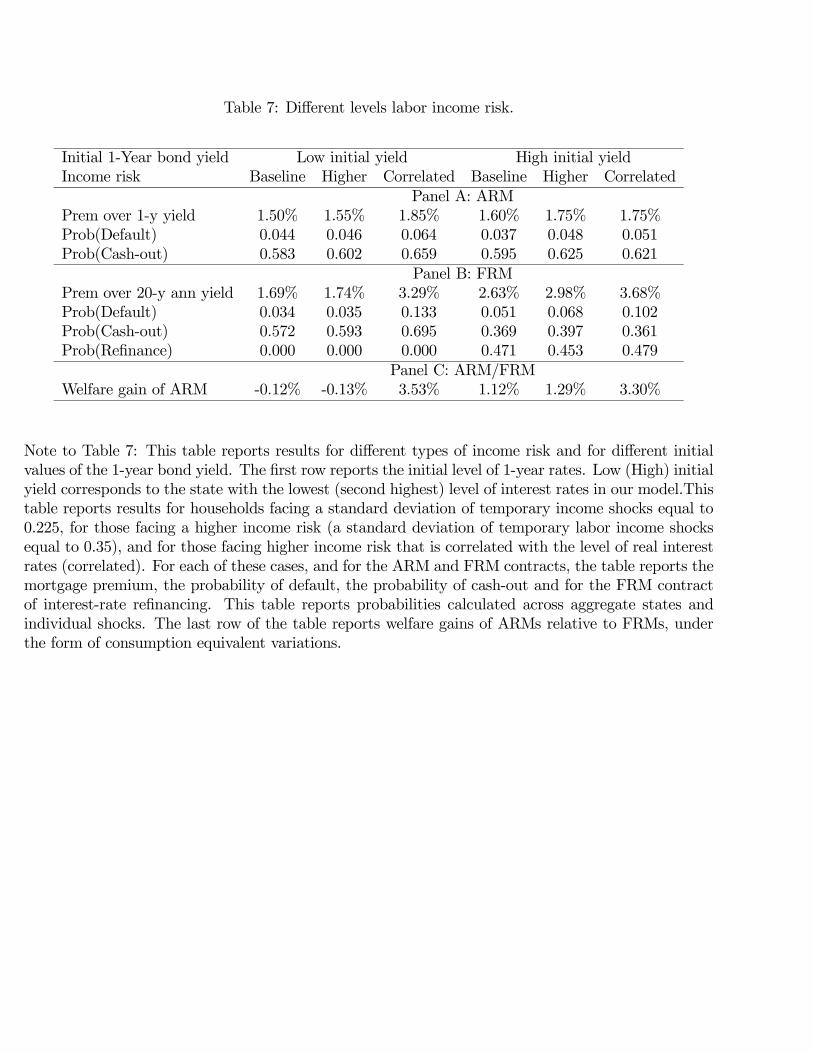
Table 7: Different levels labor income risk.
Initial 1-Year bond yield Low initial yield High initial yield
Income risk Baseline Higher Correlated Baseline Higher Correlated
Panel A: ARM
Prem over 1-y yield 1.50% 1.55% 1.85% 1.60% 1.75% 1.75%
Prob(Default) 0.044 0.046 0.064 0.037 0.048 0.051
Prob(Cash-out) 0.583 0.602 0.659 0.595 0.625 0.621
Panel B: FRM
Prem over 20-y ann yield 1.69% 1.74% 3.29% 2.63% 2.98% 3.68%
Prob(Default) 0.034 0.035 0.133 0.051 0.068 0.102
Prob(Cash-out) 0.572 0.593 0.695 0.369 0.397 0.361
Prob(Refinance) 0.000 0.000 0.000 0.471 0.453 0.479
Panel C: ARM/FRM
Welfare gain of ARM -0.12% -0.13% 3.53% 1.12% 1.29% 3.30%
Note to Table 7: This table reports results for different types of income risk and for different initial
values of the 1-year bond yield. The first row reports the initial level of 1-year rates. Low (High) initial
yield corresponds to the state with the lowest (second highest) level of interest rates in our model.This
table reports results for households facing a standard deviation of temporary income shocks equal to
0.225, for those facing a higher income risk (a standard deviation of temporary labor income shocks
equal to 0.35), and for those facing higher income risk that is correlated with the level of real interest
rates (correlated). For each of these cases, and for the ARM and FRM contracts, the table reports the
mortgage premium, the probability of default, the probability of cash-out and for the FRM contract
of interest-rate refinancing. This table reports probabilities calculated across aggregate states and
individual shocks. The last row of the table reports welfare gains of ARMs relative to FRMs, under
the form of consumption equivalent variations.

Table 8: Other household parameters.
Initial 1-Year bond yield Low initial yield High initial yield
Parameter Baseline Inc growth Disc factor Mov prob Stigma Baseline Inc growth Disc factor Mov prob Stigma
Panel A: ARM
Prob(Default) 0.044 0.044 0.048 0.055 0.034 0.037 0.036 0.041 0.049 0.029
Prob(Cash-out) 0.583 0.569 0.637 0.690 0.586 0.595 0.581 0.654 0.702 0.596
Prem over 1-y yield 1.50% 1.50% 1.60% 1.70% 1.45% 1.60% 1.58% 1.75% 1.80% 1.55%
Panel B: FRM
Prob(Default) 0.034 0.034 0.034 0.042 0.025 0.051 0.051 0.052 0.061 0.040
Prob(Cash-out) 0.572 0.558 0.603 0.685 0.573 0.369 0.356 0.472 0.430 0.371
Prob(Refinance) 0.000 0.000 0.000 0.000 0.000 0.471 0.477 0.362 0.441 0.475
Prem over 20-y ann yield 1.69% 1.69% 1.72% 1.81% 1.64% 2.63% 2.63% 2.48% 2.93% 2.53%
Panel C: ARM/FRM
Welfare gain of ARM -0.12% -0.13% -0.22% -0.07% -0.14% 1.12% 1.08% 0.63% 1.27% 1.07%
Note to Table 8: This table reports results for different household parameters and for different initial
values of the 1-year bond yield. Low (High) initial yield corresponds to the state with the lowest
(second highest) level of interest rates in our model. This table reports results for households facing
the baseline parameters, for those facing a higher growth rate of labor income (equal to 0.012), for
those with a lower discount factor (equal to 0.92), and for those facing a higher probability of an
exogenous house move (equal to 0.06), and a desutility from default. For each of these cases, and for
the ARM and FRM contracts, the table reports the mortgage premium, the probability of default,
the probability of cash-out and for the FRM contract of interest-rate refinancing. This table reports
probabilities calculated across aggregate states and individual shocks. The table reports welfare gains
of ARMs relative to FRMs, under the form of consumption equivalent variations.

Table 9: ARM contract with a teaser rate and lower target profitability.
Initial 1-Year bond yield Low initial yield High initial yield
Profitability Baseline Lower Baseline Lower
Panel A: ARM
Prem over 1-y yield 1.50% 1.25% 1.60% 1.30%
Prob(Default) 0.044 0.041 0.037 0.034
Prob(Cash-out) 0.583 0.582 0.595 0.592
Panel B: FRM
Prem over 20-y ann yield 1.69% 1.44% 2.63% 2.18%
Prob(Default) 0.034 0.031 0.051 0.045
Prob(Cash-out) 0.572 0.570 0.369 0.368
Prob(Refinancing) 0.000 0.000 0.471 0.471
Panel C: ARM Teaser
Prem over 1-y yield 0%/1.75% 0%/1.85%
Prob(Default) 0.046 0.040
Prob(Cash-out) 0.584 0.596
Panel D: ARM/FRM/ARM Teaser
Welfare gain of ARM/FRM -0.12% -0.10% 1.12% 1.04%
Welf gain ARM /ARM Teaser 0.09% -0.04%
Note to Table 9: This table reports results for different levesl of lender profitability (equal to 0.08)
and for an ARM with a teaser rate, for different initial values of the 1-year bond yield. Low (High)
initial yield corresponds to the state with the lowest (second highest) level of interest rates in our
model. The ARM contract with a teaser rate has a interest rate equal to the 1-year bond yield for
the first year of the contract, that is reset to a higher value in subsequent years. This table reports
probabilities calculated across aggregate states and individual shocks. The last row of the table reports
welfare gains of ARMs relative to FRMs, and of ARMs relative to the ARM teaser under the form of
consumption equivalent variations.

Table 10: Cumulative probabilities of default, cash-out and refinance, by mortgage type and income
risk characteristics, for a path of the aggregate variables that matches the U.S. experience.
Prob through end 2006 Year mort 2005 Year mort 2006
ARM Cash-out Default Default
Base case 0.078 0.000 0.008
Higher inc risk 0.106 0.000 0.008
Correl inc risk 0.078 0.000 0.008
FRM Refinance Cash-out Default Default
Base case 0.000 0.078 0.000 0.008
Higher inc risk 0.000 0.164 0.000 0.008
Correl inc risk 0.000 0.078 0.000 0.008
Prob through end 2007 Year mort 2005 Year mort 2006
ARM Cash-out Default Default
Base case 0.115 0.000 0.016
Higher inc risk 0.159 0.000 0.060
Correl inc risk 0.216 0.000 0.016
FRM Refinance Cash-out Default Default
Base case 0.755 0.115 0.000 0.016
Higher inc risk 0.677 0.198 0.000 0.060
Correl inc risk 0.000 0.166 0.000 0.278
Prob through end 2008 Year mort 2005 Year mort 2006
ARM Cash-out Default Default
Base case 0.115 0.008 0.023
Higher inc risk 0.159 0.007 0.067
Correl inc risk 0.216 0.030 0.023
FRM Refinance Cash-out Default Default
Base case 0.755 0.115 0.001 0.023
Higher inc risk 0.677 0.198 0.009 0.067
Correl inc risk 0.000 0.166 0.246 0.937
Prob through end 2009 Year mort 2005 Year mort 2006
ARM Cash-out Default Default
Base case 0.115 0.015 0.032
Higher inc risk 0.159 0.014 0.075
Correl inc risk 0.216 0.044 0.032
FRM Refinance Cash-out Default Default
Base case 0.755 0.115 0.002 0.032
Higher inc risk 0.677 0.198 0.010 0.087
Correl inc risk 0.000 0.166 0.289 1.000
Note to Table 10: This table reports the probabilities of default, cash-out and refinancing for a given
path of the aggregate variables, that match the U.S. historical experience. The table reports results
for LTI=4.5 and LTV = 0.90, for different household income risk characteristics, and for mortgages
that began in 2005 and in 2006.

Table 11: Mortgage premia in the data and in the model.
1-year bond yield <0.021 0.021 to 0.041 0.041 to 0.061 >0.061
Panel A.1: Premium in the data, based on 1-year bond yield
ARM premium 3.80% 2.59% 1.55% 1.27%
FRM premium 1.58% 1.53% 1.55% 1.89%
Term structure slope > 0.016 0.0 to 0.016 -0.016 to 0 <-0.016
Panel A.2: Premium in the data, based on slope of term structure
ARM premium 2.78% 1.45% 0.82% -
FRM premium 1.56% 1.71% 2.09% -
Panel B.1: ARM Premium in the model
Baseline 1.50% 1.60% 1.60% 1.70%
Lower LTV 1.45% 1.55% 1.55% 1.75%
Higher inc risk 1.55% 1.65% 1.75% 1.95%
Correlated inc risk 1.85% 1.70% 1.75% 1.65%
Lower profitability 1.25% 1.30% 1.30% 1.40%
Panel B.2: FRM Premium in the model
Baseline 1.69% 2.26% 2.63% 4.69%
Lower LTV 1.64% 1.72% 2.28% 3.39%
Inertia = 0.5 1.69% 1.66% 2.18% 2.99%
Lower profitability 1.44% 1.71% 2.18% 3.59%
Note to Table 11: Panel A.1 and A.2 report the average ARM and FRM premia in the data for different
levels of the 1-year bond yield and of the slope of the term structure of interest rates. The data are
from the Monthly Interest Rate Survey from 1986.01 to 2008.10. Panels B.1 (B.2) reports some of the
model predicted mortgage premia for ARMs (FRMs).

Table 12: Predicting mortgage premia.
Independent variables (1) ARM (2) ARM (3) FRM (4) FRM
Yield on 1-year zero coupon bonds -0.409 -0.415 0.045 0.189
[0.019] [0.016] [0.012] [0.022]
Yield on 20-year annuity -0.227
[0.029]
LTV for ARM - FRM 0.119 0.130 -0.074 -0.066
[0.038] [0.015] [0.019] [0.017]
LTV for ARM -0.187
[0.020]
LTV for FRM -0.086 -0.108
[0.015] [0.142]
Number of observations 274 274 274 274
Adjusted R-squared 0.671 0.75 0.136 0.292
Note to Table 12: The dependent variable is the mortgage premia for ARMs (specifications (1) and
(2)) and for FRMs (specifications (3) and (4)). Standard errors are reported in parenthesis below the
estimated coefficients. The data are monthly from 1986.01 to 2008.10. The yields data are from the
Federal Reserve Board. The mortgage related data are from the Monthly Interest Rate Survey. The
variable LTV for ARM-FRM is the difference in LTV between ARM and FRM mortgages that are
initiated during the month (in percentage points). All regressions include a constant (not reported).