10

International Journal of Golf Science, 2012, 1, 10-24 © 2012 Human Kinetics, Inc.

The authors are with Lehrstuhl für Traininsgwissenschaft und Sportinformatik, Technische Universität München, Munich, Germany.

A Model for Visualizing Difficulty in Golf and Subsequent Performance

Rankings on the PGA Tour

Michael Stöckl, Peter F. Lamb, and Martin LamesTechnische Universität München

Conventional performance indicators used in golf tend to rely on classifications of shots based on the distance to the hole. Consequently, these indicators ignore the unique factors which make up the difficulty of each shot. The aim of the project was to develop new performance indicators which are independent from the other shots played on a hole as well as a visualization of unique areas on a hole. Using the ISOPAR method a representative performance of the field is calculated at each hole. This allows visualizing difficult areas with respect to the field’s performance and new performance indicators which are independent of preceding shots. We looked at the ShotLink database for all tournaments measured in 2011 and com-pared the rankings of the PGA Tour to rankings generated using the ISOPAR method. We argue that the players who do well in the ISOPAR based rankings tend to be players who are subjectively and popularly known to be good performers for the respective shot types. The theoretical background and anecdotal evidence are used as support for the ISOPAR method’s ability to analyze the performance of individual shots in golf.

Keywords: modeling; golf; performance analysis

Performance analysis characterizes processes in sport by describing how an outcome was attained to measure performance itself (Hughes & Bartlett, 2002). In doing so, indicators for performance are defined. In golf, classical performance analysis has focused on analyzing classes of shots (James, 2007) like driving distance, approach shot accuracy or putting average (James & Rees, 2008). Per-formance indicators like average putts per green, driving distance or greens in regulation are designated for analyzing players’ abilities in performing certain types of shots. However, these measures do not only describe a specific ability of the player but many abilities of the player. For example, the starting position of a player’s first putt on the green is determined by the approach shot. Hence, a player who performs approach shots well, as a consequence, tends to experience easier putts. Furthermore, the starting position of the approach shot is the result of

The ISOPAR Method 11

the previous shot. Therefore, putting average is a composite measure since it not only describes putting ability but also the performance of all previous shots on a hole. For this reason, to identify players’ strengths and weaknesses, independent measures of performance for certain types of shots must be developed (Ketzscher & Ringrose, 2002). Currently, there is only one performance indicator, the newly developed indicator strokes gained (Broadie, 2011; Fearing, Acimovic & Graves, 2011), which accounts for the influence one shot has on the next. As suggested above, each shot on a hole is part of a chain of events which starts at the tee and ends when the ball is holed out. Except for the tee shot, the starting conditions of a shot are the result of the finishing position of the previous shot. Hence, a model which includes environmental conditions and the stroke sequence is more suitable than analyzing frequencies of discrete events.

The lack of this sort of performance indicator was also recognized by other research groups (Broadie, 2008; Broadie, 2011; Fearing et al., 2011; Landsberger, 1994). These groups developed statistical models which provide probabilities of holing out with respect to the distance to the pin. The development of such statisti-cal benchmarks is based on an idea of Cochran and Stobbs (1968) who manually collected data, albeit a small dataset, and calculated probabilities of holing out from certain distances on the green and the respective remaining average number of shots until the ball was holed from these distances. At the time of their study they were prevented from developing this idea by lack of modern computer technology to collect and analyze data. Broadie (2008) developed this idea further and defined a measurement for individual strokes, a shot value system strokes gained, based on different statistical benchmarks on and off the green (Broadie, 2011). Fearing et al. (2011) worked out a similar statistical model to predict the number of remaining shots to hole out based on the distance to the hole on the green, difficulty of the green, and the performance of the participating golfers. Their performance indica-tor, Strokes Gained—Putting, is based on Broadie’s idea (2008) and is used as the first official measurement for individual shots by the PGA Tour.

Whereas these approaches are statistical and developed to predict performance and eventually compare performance to expected benchmarks, our working group took a different approach, which is specifically aimed at characterizing the perfor-mance of the participating golfers, rather than predicting it. We call the model the ISOPAR method (Stöckl, Lamb & Lames, 2011). The approach of the ISOPAR project comes from a systems perspective which has been empirically applied to many levels of analysis of human movement and performance (e.g., Davids et al. (2003); Kelso (1995); Mayer-Kress et al. (2006)). The central concept is that neurobiological systems behave as complex systems and theories from physical sciences, e.g., dynamical systems theory, are appropriate for understanding and mod-eling human performance. We extended this perspective to golf performance on the PGA Tour measured by ShotLink. The underlying assumption is that each shot a player faces, represents a new set of constraints and the player must adapt to the constraints associated with the shot, which can be divided into three main categories: environment, organism, task (Newell, 1986). We have already shown in a previous study that the ISOPAR method is suitable to visualize constraints in putting (Stöckl & Lames, 2011). This idea can be extended to entire holes to illustrate difficulty on a hole represented by the number of remaining shots, since each shot is part of a player’s shot sequence. Hence, a representation of the performance of the participating golfers is calculated,

12 Stöckl, Lamb, and Lames

according to the number of remaining shots, for a hole and a specific pin position by the ISOPAR method. Based on that, the ISOPAR method provides a) a visualization of unique areas on a hole with respect to the participating players and a certain pin position and b) a performance indicator for individual shots, Shot Quality, which describes the quality of a shot with respect to the difficulty of its starting location and its finishing location. Using the ISOPAR method we analyzed the PGA Tour ShotLink data from all measured tournaments in 2011.

MethodsIn this section the concept on which the ISOPAR method is based will be explained. Furthermore, the different steps of the algorithm of the ISOPAR method will be described.

The Concept

The idea of the ISOPAR method is based on and can be explained well by an anal-ogy to isobar maps used in meteorology. In meteorology, isobar maps visualize barometric pressure by plotting lines of equal pressure, the isobar lines (iso—means equal; bar—means pressure), on geographical maps. Minima and maxima, which are areas of low and high air pressure respectively, can be identified by closed lines with usually a small diameter. Closely packed lines represent a large change in pressure and spread out lines represent a small change in pressure. Similarly, the ISOPAR method was developed to calculate and visualize difficulty on golf holes and the changes in difficulty. By plotting the values on a map of a golf hole unique areas can be identified. We call these maps ISOPAR maps.

Data and the ISOPAR Algorithm

The calculation of ISOPAR values and ISOPAR maps is based on information about shots. The ISOPAR method needs as input arguments the ball locations and the number of remaining shots from each ball location. In this study we used information about all shots (n = 1,009,362) measured by ShotLink from 38 PGA Tour tournaments in 2011 to calculate ISOPAR values and ISOPAR maps for 2,754 holes played in 153 rounds.

The ISOPAR values and ISOPAR maps are calculated in three and four steps, respectively. The ISOPAR method was programmed with MATLAB R2011b using common MATLAB procedures for some of the steps. More details of the method are explained in Stöckl et al. (2011). Although the algorithm is described only with respect to the green in Stöckl et al. (2011), the analysis in the current study is based on the same algorithm for calculating ISOPAR values and the corresponding maps for entire holes; therefore, only a summary of the steps is provided.

1. A two dimensional grid is assigned to the hole. This gives us a set of grid nodes represented by pairs (xij, yij), i = 1, ..., m, j = 1, ..., n. In this study a grid size of two inches was used.

2. At the grid nodes ISOPAR values zij are calculated. This calculation is based on the ball locations and the respective number of remaining shots at the ball

The ISOPAR Method 13

locations. The ISOPAR value calculation at any grid node considers all ball locations which are in an area 60 degrees left and 60 degrees right of the straight line between hole and this grid node (vertex being the hole). This angle was decided upon so that ball locations beyond the hole do not influence the calcu-lation. The included ball locations are then sorted in ascending order by their Euclidean distanced dijp, p = 1, ..., q (q = number of included ball locations) to the respective grid node. In the resulting order, (dijr, zr) represents the ball location with the shortest distance to grid node (xij,yij) and (dij1, z1) represents the ball location with the greatest distance to the grid node (xij,yij).

The ISOPAR value zij is a representative performance of the field and is computed using an exponential smoothing algorithm (Hamilton, 1994)

∑α α α= − + −=

−

−−z z z(1 ) (1 ) ,ij

k

rk

r kr

0

21

1

where α is a smoothing parameter. In this study, α = .17 was chosen because it achieved good representativeness of each shot without giving too much influence to infrequent or outlying data.

Furthermore, to reduce computational intensity a nonconvex area was defined which contained all ball locations (for the given hole and round). ISOPAR values were only calculated at grid nodes which were located in this area.

3. Continuous, three-dimensional ISOPAR values are calculated for the entire hole by means of a spline interpolation (Fahrmeir, Kneib & Lang, 2009) based on the ISOPAR values at the grid nodes from the previous step.

To achieve a satisfactorily smooth surface, a slightly smoothing, cubic spline interpolant ƒ(x, y) is calculated by

∑∑ ∫∫β β λ )()( )(− + −= =

z f v D f x y dx dymin  ( ( )) 1 , ,f

i

n

j

m

ij ij1 1

2 2 2

where

=∂

∂+

∂∂ ∂

+∂

∂D

x x y y2 ,2

2

2

2 2

2

νij denotes the vector with entries yij

xij( ) (the coordinates of the grid nodes) λ = 1 in our case and β is the smoothing parameter. In this study we used 0.98 as smoothing parameter.

4. Based on the continuous ISOPAR values so called iso-lines are calculated for certain levels. In this study we calculated iso-lines at intervals of 0.2 ISOPAR value. For example, the iso-line at interval 1.8 is calculated as the intersection line between the ISOPAR surface of step 3 and the plane which is parallel to the x-y-plane with a distance of 1.8 ISOPAR value by

xy

f v( )

⎛

⎝

⎜⎜⎜⎜⎜⎜⎜⎜

⎞

⎠

⎟⎟⎟⎟⎟⎟⎟⎟⎟=

00

1.8

⎛

⎝

⎜⎜⎜⎜⎜⎜⎜

⎞

⎠

⎟⎟⎟⎟⎟⎟⎟⎟+

100

⎛

⎝

⎜⎜⎜⎜⎜⎜⎜

⎞

⎠

⎟⎟⎟⎟⎟⎟⎟⎟+J

010

⎛

⎝

⎜⎜⎜⎜⎜⎜⎜

⎞

⎠

⎟⎟⎟⎟⎟⎟⎟⎟,

where ν denotes the vector with entries yx( ) and μ, ϑ ε . Finally, an ISOPAR map

is created by plotting the iso-lines on a map of a hole.

μ

14 Stöckl, Lamb, and Lames

The ISOPAR value at the tee was defined as the average hole score for the respective round. Since there were ISOPAR values smaller than 1 for a few holes the three-dimensional ISOPAR surface was lifted so that the smallest ISOPAR value became 1.

ResultsGenerally, the ISOPAR method provides two results. First, the difficulty of holes can be calculated and visualized by ISOPAR maps. Second, the ISOPAR method provides performance indicators by which the performance of any shot can be analyzed with respect to its difficulty which is determined by the performance of the field. These two results will be outlined in this section with respect to data from the PGA Tour collected by ShotLink.

ISOPAR Maps

In Stöckl et al. (2011) the concept of ISOPAR maps was originally described for on-green performance of amateur golfers. In this study we extended the idea of calculating and visualizing difficulty to off-green performance and applied it to the performance of PGA Tour golfers. According to Stöckl and Lames (2011) ISOPAR maps are suitable for identifying unique areas on the green. The iso-lines represent different levels of difficulty according to the number of remaining shots required to hole out. For example, if iso-lines were spread out evenly and circularly, we could conclude that all the constraints which influence performance were evenly distrib-uted. Yet, we know that many factors (e.g., distance to the hole, angle of approach, distance of the hole from the front of the green, speed and hardness of greens, etc.) directly influence performance, but they also indirectly influence performance. In other words, having a tree blocking the line to the pin constrains the kind of shot a player can play. This is an example of that factor directly affecting performance.

An example of a factor indirectly affecting performance is a situation in which a player tries to play strategically, by aiming away from a hazardous area. The shot might result in a long remaining putt but has essentially eliminated the possibility of going in the hazard. The strength of the ISOPAR method is its capability of accounting for all the factors which influence performance. To illustrate this idea further, imagine all the players on a hole aim at a certain area of the green rather than the pin because the pin is close to a penalizing hazard. This would affect the distance-based statistical benchmarks and would make it look like everyone per-formed worse than expected. Accordingly, the benchmark could then be adjusted so that it is only representative of shots played on that specific hole. To take this example one step further, imagine a situation in which long hitters give themselves such an advantage off the tee that they can play to the pin whereas the rest of the field still feel wise to play more conservatively. This situation represents a nonlinear relationship between players’ strategies. The same example is easy to think of on risk reward holes such as drivable par-4s and tricky par-5s. The ISOPAR method is capable of modeling these nonlinearities in the data because it is a measure of per-formance rather than a predictor. The ISOPAR maps are capable of identifying how advantageous shots were (e.g., a drive that provides a good angle for the approach shot) as well as how hazardous hazards were (e.g., rough, bunkers, trees, etc.).

The ISOPAR Method 15

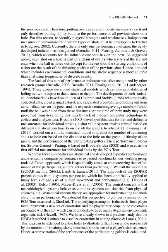
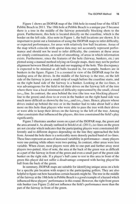
Figure 1 shows an ISOPAR map of the 18th hole in round four of the AT&T Pebble Beach in 2011. The 18th hole at Pebble Beach is a unique par-5 because there is a tree in the middle of the fairway potentially blocking shots to the green. Furthermore, this hole is located directly on the coastline, which is the border on the left side. Also note in Figure 1, the ball locations are shown. It is important to point out a limitation of using the ISOPAR maps to infer difficulty, or expected performance, for areas with relatively few ball locations. Areas of the map which coincide with sparse data may not accurately represent perfor-mance and should not be used to infer difficulty, the contours at these areas are simply continuations, as result of smoothing, of areas in which information exists. Furthermore, since the features of the hole (fairway, bunkers, etc.) are plotted using a manual method relying on Google maps, there may not be perfect alignment between ShotLink data and our mapping of the hole. This discrepancy is expected to be minimal as all balls located in, for example, bunkers are in bunkers in the figure. Figure 2 is a zoomed in view of the ISOPAR map for the landing area of the drives. In the middle of the fairway is the tree, on the left side of the fairway is just a small strip of rough before the coastline starts, and on the right hand side of the fairway is a bunker. Looking at the iso-lines, it was advantageous for the field to hit their drives on the fairway left of the tree where there was a local minimum of difficulty represented by the small, closed iso3.6 line. In contrast, the area behind the tree (the tree was blocking players’ line to the green) and close to or even in the bunker on the right hand side was much more difficult as shown by the iso4.0 and iso4.2 lines. Hence, players whose drives ended up behind the tree or in the bunker had to take about half a shot more on this hole than players who were able to pass the tree with their drives or were able to keep their drives on the fairway to the left of the tree. Among other constraints that influenced the players, this tree constrained the field’s play significantly.

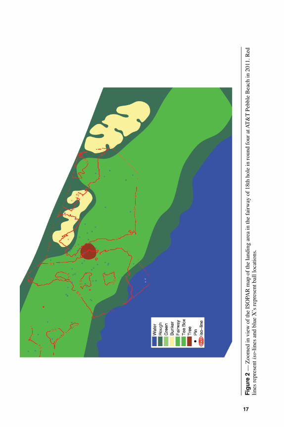
Figure 3 illustrates another zoom on a part of the ISOPAR map, the green and the area around it. As already outlined in Stöckl et al. (2011), iso-lines on the green are not circular which indicates that the participating players were constrained dif-ferently and to different degrees depending on the line they approached the hole from. Around the hole there is a noticeably more densely packed band of iso-lines. These lines represent an area of increased variability in performance—many players were one-putting while others were two-putting. In contrast, other areas were less variable. When closer, most players were able to one-putt and further away most players two-putted. Also of note, the area at the back of the green was as difficult as a part of the fairway in front of the green and even a small part of the green side bunker on the right side. If a player’s ball came to rest in this area in front of the green this player did not suffer a disadvantage compared with having played his ball from the back of the green.

In summary, ISOPAR maps are suitable for identifying unique areas on a hole for a specific pin location with respect to the participating golfers. They are also helpful to figure out how hazardous certain hazards might be. The tree in the middle of the fairway at the 18th hole in Pebble Beach is a good example of a hazard which influenced these players’ performance in this round. However, the right front green side bunker (see Figure 2) did not influence the field’s performance more than the part of the fairway in front of the green.

16

Fig

ure

1 —

ISO

PAR

map

of 1

8th

hole

of r

ound

four

at A

T&

T P

ebbl

e B

each

in 2

011.

Red

line

s re

pres

ent i

so-l

ines

and

blu

e X

’s re

pres

ent b

all l

ocat

ions

.

17

Fig

ure

2 —

Zoo

med

in v

iew

of

the

ISO

PAR

map

of

the

land

ing

area

in th

e fa

irw

ay o

f 18

th h

ole

in r

ound

fou

r at

AT

&T

Peb

ble

Bea

ch in

201

1. R

ed

lines

rep

rese

nt is

o-lin

es a

nd b

lue

X’s

rep

rese

nt b

all l

ocat

ions

.

18

Fig

ure

3 —

Zoo

med

in

view

of

the

ISO

PAR

map

of

the

18th

gre

en a

nd t

he a

rea

arou

nd i

t fr

om r

ound

fou

r at

AT

&T

Peb

ble

Bea

ch i

n 20

11. R

ed

lines

rep

rese

nt is

o-lin

es a

nd b

lue

X’s

rep

rese

nt b

all l

ocat

ions

.

The ISOPAR Method 19

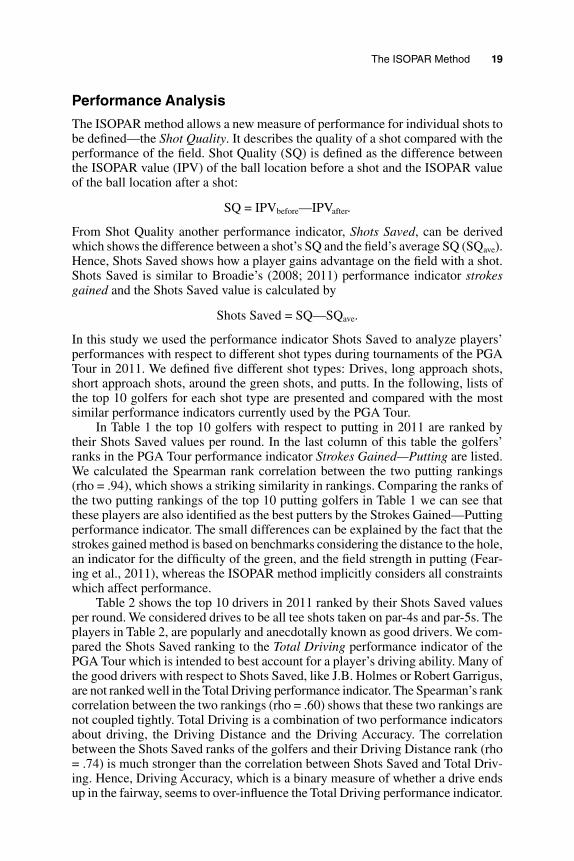
Performance Analysis

The ISOPAR method allows a new measure of performance for individual shots to be defined—the Shot Quality. It describes the quality of a shot compared with the performance of the field. Shot Quality (SQ) is defined as the difference between the ISOPAR value (IPV) of the ball location before a shot and the ISOPAR value of the ball location after a shot:

SQ = IPVbefore—IPVafter.

From Shot Quality another performance indicator, Shots Saved, can be derived which shows the difference between a shot’s SQ and the field’s average SQ (SQave). Hence, Shots Saved shows how a player gains advantage on the field with a shot. Shots Saved is similar to Broadie’s (2008; 2011) performance indicator strokes gained and the Shots Saved value is calculated by

Shots Saved = SQ—SQave.

In this study we used the performance indicator Shots Saved to analyze players’ performances with respect to different shot types during tournaments of the PGA Tour in 2011. We defined five different shot types: Drives, long approach shots, short approach shots, around the green shots, and putts. In the following, lists of the top 10 golfers for each shot type are presented and compared with the most similar performance indicators currently used by the PGA Tour.

In Table 1 the top 10 golfers with respect to putting in 2011 are ranked by their Shots Saved values per round. In the last column of this table the golfers’ ranks in the PGA Tour performance indicator Strokes Gained—Putting are listed. We calculated the Spearman rank correlation between the two putting rankings (rho = .94), which shows a striking similarity in rankings. Comparing the ranks of the two putting rankings of the top 10 putting golfers in Table 1 we can see that these players are also identified as the best putters by the Strokes Gained—Putting performance indicator. The small differences can be explained by the fact that the strokes gained method is based on benchmarks considering the distance to the hole, an indicator for the difficulty of the green, and the field strength in putting (Fear-ing et al., 2011), whereas the ISOPAR method implicitly considers all constraints which affect performance.

Table 2 shows the top 10 drivers in 2011 ranked by their Shots Saved values per round. We considered drives to be all tee shots taken on par-4s and par-5s. The players in Table 2, are popularly and anecdotally known as good drivers. We com-pared the Shots Saved ranking to the Total Driving performance indicator of the PGA Tour which is intended to best account for a player’s driving ability. Many of the good drivers with respect to Shots Saved, like J.B. Holmes or Robert Garrigus, are not ranked well in the Total Driving performance indicator. The Spearman’s rank correlation between the two rankings (rho = .60) shows that these two rankings are not coupled tightly. Total Driving is a combination of two performance indicators about driving, the Driving Distance and the Driving Accuracy. The correlation between the Shots Saved ranks of the golfers and their Driving Distance rank (rho = .74) is much stronger than the correlation between Shots Saved and Total Driv-ing. Hence, Driving Accuracy, which is a binary measure of whether a drive ends up in the fairway, seems to over-influence the Total Driving performance indicator.

20 Stöckl, Lamb, and Lames

Table 1 Top 10 Putters in 2011 Ranked by Shots Saved Values Per Round. Last Column Contains Rank in PGA Performance Indicator Strokes Gained—Putting.

Rank NameRounds Measured

Shots SavedPer Round

Shots SavedTotal

Strokes GainedRank (PGA)

1. Bryce Molder 71 0.773 54.863 3

2. Luke Donald 52 0.751 39.043 1

3. Charlie Wi 77 0.734 56.506 4

4. Steve Stricker 53 0.716 37.972 2

5. Kevin Na 68 0.591 40.159 8

6. Fredrik Jacobson 70 0.573 40.090 6

7. Brandt Snedeker 67 0.555 37.174 10

8. Greg Chalmers 79 0.553 43.668 5

9. Hunter Mahan 76 0.551 41.869 13

10. Jason Day 59 0.534 31.497 7

N = 202

Table 2 Top 10 Drivers in 2011 Ranked by Shots Saved Values Per Round. Last Two Columns Contain Ranks in PGA Performance Indicator Total Driving and Driving Distance.

Rank NameRounds Measured

Shots SavedPer Round

Shots SavedTotal

Total DrivingRank (PGA)

Driving Distance Rank (PGA)

1. J. B. Holmes 47 0.991 46.588 90 1

2. Dustin Johnson 54 0.904 48.827 30 3

3. Gary Woodland 70 0.834 58.382 23 5

4. Robert Garrigus 69 0.787 54.317 94 4

5. Bubba Watson 59 0.780 46.003 35 2

6. Adam Scott 45 0.710 31.972 5 24

7. Jhonattan Vegas 70 0.595 41.644 84 8

8. Martin Laird 62 0.572 35.435 26 13

9. Bill Haas 72 0.566 40.745 76 48

10. Kyle Stanley 80 0.558 44.653 18 9

N = 202

The ISOPAR Method 21

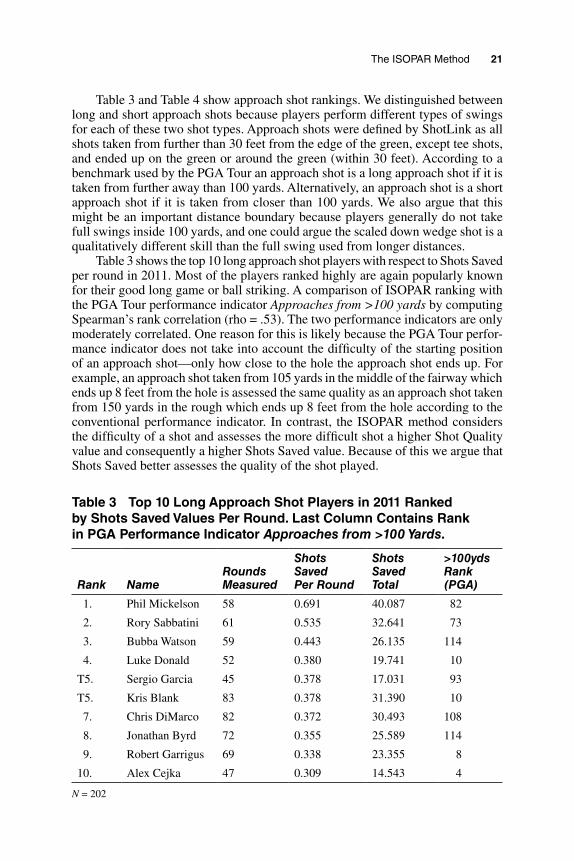
Table 3 and Table 4 show approach shot rankings. We distinguished between long and short approach shots because players perform different types of swings for each of these two shot types. Approach shots were defined by ShotLink as all shots taken from further than 30 feet from the edge of the green, except tee shots, and ended up on the green or around the green (within 30 feet). According to a benchmark used by the PGA Tour an approach shot is a long approach shot if it is taken from further away than 100 yards. Alternatively, an approach shot is a short approach shot if it is taken from closer than 100 yards. We also argue that this might be an important distance boundary because players generally do not take full swings inside 100 yards, and one could argue the scaled down wedge shot is a qualitatively different skill than the full swing used from longer distances.

Table 3 shows the top 10 long approach shot players with respect to Shots Saved per round in 2011. Most of the players ranked highly are again popularly known for their good long game or ball striking. A comparison of ISOPAR ranking with the PGA Tour performance indicator Approaches from >100 yards by computing Spearman’s rank correlation (rho = .53). The two performance indicators are only moderately correlated. One reason for this is likely because the PGA Tour perfor-mance indicator does not take into account the difficulty of the starting position of an approach shot—only how close to the hole the approach shot ends up. For example, an approach shot taken from 105 yards in the middle of the fairway which ends up 8 feet from the hole is assessed the same quality as an approach shot taken from 150 yards in the rough which ends up 8 feet from the hole according to the conventional performance indicator. In contrast, the ISOPAR method considers the difficulty of a shot and assesses the more difficult shot a higher Shot Quality value and consequently a higher Shots Saved value. Because of this we argue that Shots Saved better assesses the quality of the shot played.

Table 3 Top 10 Long Approach Shot Players in 2011 Ranked by Shots Saved Values Per Round. Last Column Contains Rank in PGA Performance Indicator Approaches from >100 Yards.

Rank NameRounds Measured

Shots SavedPer Round

Shots SavedTotal

>100ydsRank (PGA)

1. Phil Mickelson 58 0.691 40.087 82

2. Rory Sabbatini 61 0.535 32.641 73

3. Bubba Watson 59 0.443 26.135 114

4. Luke Donald 52 0.380 19.741 10

T5. Sergio Garcia 45 0.378 17.031 93

T5. Kris Blank 83 0.378 31.390 10

7. Chris DiMarco 82 0.372 30.493 108

8. Jonathan Byrd 72 0.355 25.589 114

9. Robert Garrigus 69 0.338 23.355 8

10. Alex Cejka 47 0.309 14.543 4

N = 202

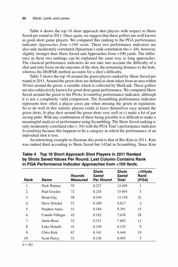
22 Stöckl, Lamb, and Lames

Table 4 shows the top 10 short approach shot players with respect to Shots Saved per round in 2011. Once again, we suggest that these golfers are well known as good short game players. We compared this ranking to the PGA performance indicator Approaches from <100 yards. These two performance indicators are also only moderately correlated (Spearman’s rank correlation rho = .68), however, slightly stronger than Shots Saved and Approaches from >100 yards. The differ-ence in these two rankings can be explained the same way as long approaches. The classical performance indicators do not take into account the difficulty of a shot and only focus on the outcome of the shot, the remaining distance to the hole, whereas the ISOPAR method accounts for a shot’s difficulty.

Table 5 shows the top 10 around the green players ranked by Shots Saved per round in 2011. Around the green shots are defined as shots taken from an area within 30 feet around the green, a variable which is collected by ShotLink. These golfers are also subjectively known for good short game performance. We compared Shots Saved around the green to the PGAs Scrambling performance indicator, although it is not a completely valid comparison. The Scrambling performance indicator represents how often a player saves par when missing the green in regulation. So to do well in this statistic players could a) leave themselves easy around the green shots, b) play their around the green shots very well or c) make a lot of par saving putts. With any combination of these being possible it is difficult to make a meaningful analysis of performance using Scrambling. The Shots Saved ranking is only moderately correlated (rho = .54) with the PGA Tour’s performance indicator Scrambling because this happens to be a category in which the performance of an individual shot is lost.

An interesting example to illustrate this point is that of Bio Kim in 2011. Kim was ranked third according to Shots Saved but 142nd in Scrambling. Since Kim

Table 4 Top 10 Short Approach Shot Players in 2011 Ranked by Shots Saved Values Per Round. Last Column Contains Rank in PGA Performance Indicator Approaches from <100 Yards.

Rank NameRounds Measured

Shots SavedPer Round

Shots SavedTotal

<100ydsRank (PGA)

1. Nick Watney 55 0.227 12.495 1

2. Paul Goydos 72 0.218 15.693 5

3. Brian Gay 58 0.194 13.159 22

4. Steve Stricker 51 0.189 9.617 2

5. Stephen Ames 51 0.184 9.391 15

6. Camilo Villegas 42 0.182 7.638 28

7. Justin Rose 51 0.151 7.693 11

8. Luke Donald 41 0.149 6.125 9

9. Chris Kirk 67 0.141 9.444 19

10. Scott Piercy 51 0.136 6.955 3

N = 202

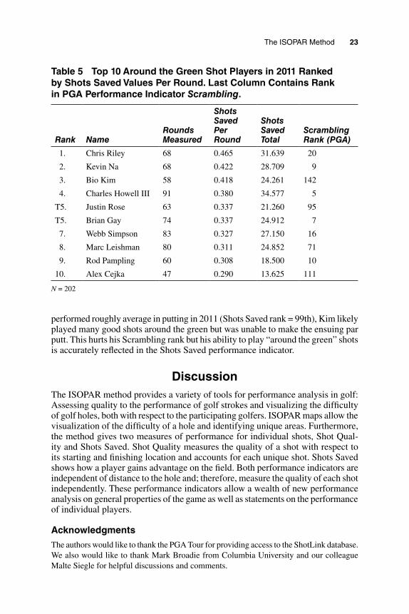
The ISOPAR Method 23

Table 5 Top 10 Around the Green Shot Players in 2011 Ranked by Shots Saved Values Per Round. Last Column Contains Rank in PGA Performance Indicator Scrambling.

Rank NameRounds Measured

Shots SavedPer Round

Shots SavedTotal

ScramblingRank (PGA)

1. Chris Riley 68 0.465 31.639 20

2. Kevin Na 68 0.422 28.709 9

3. Bio Kim 58 0.418 24.261 142

4. Charles Howell III 91 0.380 34.577 5

T5. Justin Rose 63 0.337 21.260 95

T5. Brian Gay 74 0.337 24.912 7

7. Webb Simpson 83 0.327 27.150 16

8. Marc Leishman 80 0.311 24.852 71

9. Rod Pampling 60 0.308 18.500 10

10. Alex Cejka 47 0.290 13.625 111

N = 202

performed roughly average in putting in 2011 (Shots Saved rank = 99th), Kim likely played many good shots around the green but was unable to make the ensuing par putt. This hurts his Scrambling rank but his ability to play “around the green” shots is accurately reflected in the Shots Saved performance indicator.

DiscussionThe ISOPAR method provides a variety of tools for performance analysis in golf: Assessing quality to the performance of golf strokes and visualizing the difficulty of golf holes, both with respect to the participating golfers. ISOPAR maps allow the visualization of the difficulty of a hole and identifying unique areas. Furthermore, the method gives two measures of performance for individual shots, Shot Qual-ity and Shots Saved. Shot Quality measures the quality of a shot with respect to its starting and finishing location and accounts for each unique shot. Shots Saved shows how a player gains advantage on the field. Both performance indicators are independent of distance to the hole and; therefore, measure the quality of each shot independently. These performance indicators allow a wealth of new performance analysis on general properties of the game as well as statements on the performance of individual players.

Acknowledgments

The authors would like to thank the PGA Tour for providing access to the ShotLink database. We also would like to thank Mark Broadie from Columbia University and our colleague Malte Siegle for helpful discussions and comments.

24 Stöckl, Lamb, and Lames

ReferencesBroadie, M. (2008). Assessing golfer performance using golfmetrics. In D. Crews & R. Lutz

(Eds.), Science and Golf V: Proceedings of the 2008 World Scientific Congress of Golf (253–262). Mesa, AZ: Energy and Motion Inc.

Broadie, M. (2011, April 8). A shot value approach to assessing golfer performance on the PGA Tour [Working Paper]. Columbia University, New York. Available from http://www.columbia.edu/~mnb2/broadie/Assets/strokes_gained_pga_broadie_20110408.pdf

Cochran, A., & Stobbs, J. (1968). The search for the perfect swing. Grass Valley, CA: The Booklegger.

Davids, K., Glazier, P., Araujo, D., & Bartlett, R. (2003). Movement systems as dynamical systems. Sports Medicine (Auckland, N.Z.), 33(4), 245–260. PubMed doi:10.2165/00007256-200333040-00001

Fahrmeir, L., Kneib, T., & Lang, S. (2009). Regression. Berlin: Springer.Fearing, D., Acimovic, J., & Graves, S. (2011). How to catch a Tiger: Understanding putting

performance on the PGA Tour. Journal of Quantitative Analysis in Sport, 7(1), article 5.Hamilton, J.D. (1994). Time series analysis. Princeton: Princeton University Press.Hughes, M.D., & Bartlett, R.M. (2002). The use of performance indicators in

performance analysis. Journal of Sports Sciences, 20, 739–754. PubMed doi:10.1080/026404102320675602

James, N. (2007). The statistical analysis of golf performance. International Journal of Sports Science & Coaching, 2(suppl. 1), 231–248. doi:10.1260/174795407789705424

James, N., & Rees, G.D. (2008). Approach shot accuracy as a performance indicator for US PGA Tour golf professionals. International Journal of Sports Science & Coaching, 3(suppl. 1), 145–160. doi:10.1260/174795408785024225

Kelso, J.A.S. (1995). Dynamic patterns: The self-organization of brain and behavior. Camebridge, MA: MIT Press.

Ketzscher, R., & Ringrose, T.J. (2002). Exploratory analysis of European Professional Golf Association statistics. Journal of the Royal Statistical Society: Series D, 51, 215–228. doi:10.1111/1467-9884.00313

Landsberger, L. (1994). A unified golf stroke value scale for quantitative stroke-by-stroke assessment. In A. J. Cochran & M. R. Farrally (Eds.), Science and Golf II: Proceedings of the World Scientific Congress of Golf (216–221). London: E & FN Spon.

Mayer-Kress, G., Liu, Y., & Newell, K.M. (2006). Complex Systems and Human Movement. Complexity, 12(2), 40–51. doi:10.1002/cplx.20151

Newell, K.M. (1986). Constraints on the development of coordination. In M.G. Wade & H.T.A. Whiting (Eds.), Motor development in children: Aspects of coordination and control (341–361). Amsterdam: Nijhoff.

Stöckl, M., Lamb, P., & Lames, M. (2011). The ISOPAR method—a new approach to per-formance analysis in golf. Journal of Quantitative Analysis in Sport, 7(1), article 10.

Stöckl, M., & Lames, M. (2011). Modeling Constraints in Putting: The ISOPAR Method. International Journal of Computer Science in Sport, 10(1), 74–81.