Embed Size (px)
Citation preview

1
015-0007
A Model for Optimizing Repairshop Capacity and Spare Parts Inventory
Pedram Sahba and Barış Balcıoğlu
Department of Mechanical and Industrial Engineering The University of Toronto
5 King’s College Road Toronto ON M5S 3G8 Canada
POMS 21st Annual Conference Vancouver, Canada
May 7 to May 10, 2010
Abstract
We develop a new repair shop/spare parts inventory model where transportation times and
costs are significant. We consider a system consisting of m manufacturing plants with identical
machines at different locations. When a machine fails, the defective component should be
repaired in a designated repair shop. This unit can be replaced immediately if a spare part is
available. Otherwise, the machine is down until a component is repaired and put back into
service. We find the optimal level of spare parts inventory at each location. We study the effect
of repair capacity pooling on the total cost of the system. We show that in some cases, repair
shop pooling is not cost efficient even if transportation costs are relatively low. We also show at
which location the centralized repair shop should be hosted to minimize overall system costs.

2
I. Introduction
Capacity pooling has been an important theme in the operations management literature. In
production/inventory systems, production capacity pooling has been shown to decrease the total
system costs (Yu, Benjaafar, and Gerchak, 2009 and the references therein). Likewise, it has
long been known that inventory pooling is beneficial (Eppen, 1979, Gerchak and He, 2003,
Benjaafar, Cooper, and Kim, 2005). However, in such models transportation times and costs are
often ignored whereas in real world, if production capacity or inventory is centralized this
usually implies transportation times and costs for different markets.
In this paper, we are exploring the effect of transportation times and costs on the benefits of
capacity pooling around a repair/maintenance shop. We study a problem where machines in
multiple fleets are subject to failure due to a single critical component. When a component fails,
it is sent to a repair shop, which is modeled as an FCFS single server queue. If there is a stock of
critical components kept as spare parts, one can install a spare component instantaneously on the
failed machine to prevent production loss. Otherwise, the failed machine is down until a repaired
component can be dispatched from the repair shop. If all machines are functional, the repaired
component is placed in the spare part inventory.
We consider two alternative systems for this problem. In the first system, each fleet has its
own repair shop and inventory, thereby; they do not incur any transportation costs or suffer from
transportation delays. In the second system, each location keeps its own inventory, yet the repair
shop with a higher capacity is centralized at one of the locations. Thus, some locations
experience transportation delays. Comparing these two systems, we try to address if repair shop
pooling is beneficial when transportation times and costs are not negligible.
3
The repair system with a centralized repair shop resembles production/inventory systems.
While the repair shop has different fleets of machines as its customer groups,
production/inventory systems have different classes of customers. However, unlike the
production/inventory systems in the repair system, the demand stream comes from a finite
number of machines and the failure rates (arrival rates of components to the repair shop) are state
dependent. Hence, production/inventory models differ from our model due to their assumption of
a constant arrival rate for each class, i.e., the arrival rate does not change due to the number of
orders in the production queue or the inventory levels.
The results of this research are important to maintenance contractors and large companies
that operate manufacturing plants at different locations and have their own repair facilities.
Currently, maintenance activities are contracted out more than they were a decade ago (Hui and
Tsang, 2004, Markeset and Kumar, 2008). These activities include repair services, spare parts
supply and logistics, etc. Consequently, a contractor needs to service customers’ equipment at
different locations. These contractors must decide whether a repair shop should be available at
each location (i.e., distributed repair systems) or a single repair shop with much higher capacity
should fix all repair jobs at a centralized location (i.e., a pooled repair system). For such a system
with a centralized repair shop, Sahba, Balcıoğlu, and Banjevic (2010) use a queueing-based
approach to explicitly model the limited repair capacity and associated randomness in the repair
time. They consider different policies and obtain the optimal base-stock levels for spare part
inventories under each policy to minimize the long-run average system cost as a time-average.
Through an extensive numerical analysis, they show that when transportation times and costs are
negligible, repair shop pooling is beneficial.

4
Our problem is an example of a queueing system with finite calling populations (see Sztrik,
2001, for a comprehensive bibliography on systems with finite populations). A simple system of
one repair shop and one spare parts inventory can be analyzed by a birth-and-death model.
However, a multi-class system with a centralized repair shop with local spare parts inventories at
each location is difficult to analyze even under first-come-first-served (FCFS) dispatching
policy. Incorporating transportation delays in this model is even more challenging. We model
this system as a closed queueing network and instead of using balance equations, we use Mean-
Value Analysis (MVA) developed by Reiser and Lavenberg, 1980, to obtain the stationary
system size distribution. MVA, similar to convolution algorithm (Buzen, 1973), is a numerical
algorithm that takes advantage of the product form property of queueing networks with certain
conditions (Jackson, 1963, Gordon and Newell, 1967, Baskett, Chandy, Muntz, and Palacios,
1975).
In this paper, we incorporate the transportation time and cost into a system with a central
repair shop operating under the FCFS dispatching policy and decentralized spare parts
inventories. We show that in some cases, repair shop pooling is not cost efficient even if
transportation costs are relatively low. If the repair shop is not hosted at the correct location, the
repair shop pooling can increase costs as well. Thus, our method can also be used in choosing the
optimal location of the central repair shop.
The rest of the paper is organized as follows. In Section 2, we define the problem. In Section
3, we define a repair system network and explain the common techniques such as convolution
algorithm and MVA to analyze a closed queueing network. In Section 4, we present our
algorithm for the system with a central repair shop in which transportation delays are not
5
negligible. The results of a numerical study to assess the performance of the system with a
pooled repair shop are presented in Section 5. We show that repair shop pooling is not always
beneficial, and the location of the repair shop plays a critical role in the overall performance of
the system. Finally, in Section 6, we conclude our study and discuss our future research
questions.
II. Repair Systems with Significant Transportation Times and Costs
We consider a system consisting of m manufacturing plants at different locations. Each
location has a fleet of machines run for production. At location , 1,2, … , , it is aimed to
have machines be functional at all times to continue production at targeted levels. These
machines use the same type of a repairable component and when this component fails the
machine also fails. When a machine fails, the defective component should be repaired in a
designated repair shop. This component can be replaced immediately if a spare part is available.
Otherwise, the machine is down until a component is repaired and installed on that machine
again. We assume that times to failure for each machine/component follow an independent
exponential distribution with possibly different rates, . The repair shop is modeled as a single
server queueing system with exponential service/repair times.
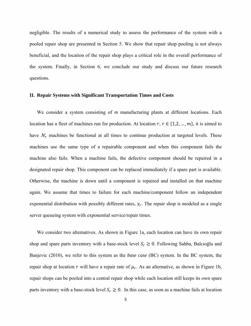
We consider two alternatives. As shown in Figure 1a, each location can have its own repair
shop and spare parts inventory with a base-stock level 0. Following Sahba, Balcıoğlu and
Banjevic (2010), we refer to this system as the base case (BC) system. In the BC system, the
repair shop at location will have a repair rate of . As an alternative, as shown in Figure 1b,
repair shops can be pooled into a central repair shop while each location still keeps its own spare
parts inventory with a base-stock level 0. In this case, as soon as a machine fails at location
6
(in fleet ), the failed component is sent to the repair shop as a type order. The repair shop
has as the repair rate and follows the FCFS policy in dispatching repaired components to
locations. This ensures that a failed component from fleet is sent back to the same fleet once its
repair is completed. In line with Sahba, Balcıoğlu and Banjevic, we refer to this system as the
decentralized FCFS (DF) system. In both systems, we exclude the possibility of transhipment of
a spare part from the positive inventory of another location.
Figure 1- The two alternative systems
Furthermore, we assume that transportation times and costs are significant in the DF system
while these do not apply to the BC system. In other words, in the DF system when a component
fails it must be transported to the repair shop, and after its repair is over it has to be brought back
to its fleet. We assume that the mean transportation time to and from the repair shop for fleet
are equal and is 1/ . In addition to the time a broken component spends in the repair shop, the
time spent in these two stages of transportation can lengthen the times machines stay down and
shorten the times inventory level is high. In other words, transportation times have an indirect
impact on the overall system cost even if only holding and down time costs are taken into
account while transportation costs are ignored. When transportation costs are ignored, letting
Spare parts inventories
Pooled repair shop
Repair orders waiting
Spare parts demand 1
Spare parts demand 2
Spare parts inventories
Repair shops Repair orders waiting
Spare parts demand 1
Spare parts demand 2
Figure 1a: Base Case (BC) system Figure 1b: Decentralized FCFS (DF) system

7
( ) denote the holding (down time) cost per spare component (per down machine) per unit time,
we have the following system cost for fleet ,
,
,
(1)
where is the steady-state probability of having components in location , and
, , … , with , which is the total number of components including spare
parts in the system at location .
Eq. (1) can be used both for the BC and DF systems; the difference is due to different
values. In the BC system, these probabilities can be found considering a simple birth-and-death
process (e.g., Gross and Harris, 1998, p. 82-83). For the DF system, to find the optimal level of
spares, an analytical method or a detailed simulation model can be employed. We have used
queueing networks concepts to obtain a fast and accurate result, which we will present in the
next section.
III. Repair Systems Network
To model the transportation delays in the DF system, we will use two infinite server queues
( / /∞) with Poisson arrivals and -stage Coxian ( ) distributions; one capturing
the time spent to take a failed component from fleet to the repair shop and the other for the
time to send a repaired component back to its fleet. An -stage Coxian random variable (r.v.)

8
(see Altiok, 1997, page 42 for more details) is a mixture of Exponential stages, i.e., a Markov
chain (MC), where each stage is indexed with j=1,…, . Starting from stage 1, with a stage
dependent probability, the MC enters the next stage or with 1 minus that probability it enters the
absorbing stage. Therefore, a Coxian distribution models the length of time spent in this MC
until one enters the absorbing stage. At the end of our analysis, only the mean value of the
Coxian distribution will be relevant. Therefore, models the one-way transportation time
between the repair shop and location and its mean will equal the mean transportation time,
1/ .
Figure 2: A single chain queueing network
The functional machines and the spare parts available at location can be modeled as an
/ / queue. Let denote the number of busy servers. When machines are operational,
any customers waiting in the queue represent the number of spare parts available. When ,
this implies that there are no spare parts and machines are down. This / / queue
for location is preceded and succeeded by the two infinite server queues modeling
transportation times. In other words, a broken component must go through the first transportation
delay to arrive at the repair shop. The repair shop is modeled as a single server queue with
exponential service times with rate . Once the component gets repaired, it returns to the original
location after passing through another transportation delay (Figure 2). The two infinite server
1
2Infinite ServerInfinite Server
Transportation Plant Transportation Repair Shop
9
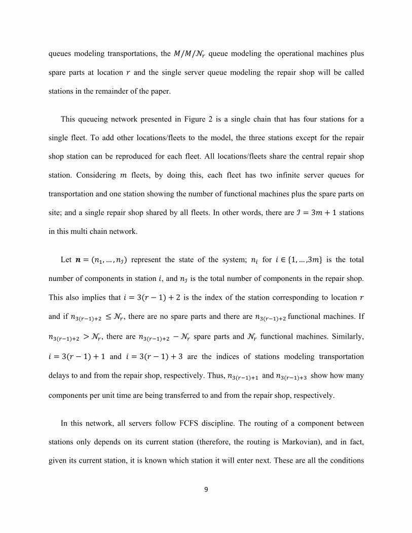
queues modeling transportations, the / / queue modeling the operational machines plus
spare parts at location and the single server queue modeling the repair shop will be called
stations in the remainder of the paper.
This queueing network presented in Figure 2 is a single chain that has four stations for a
single fleet. To add other locations/fleets to the model, the three stations except for the repair
shop station can be reproduced for each fleet. All locations/fleets share the central repair shop
station. Considering fleets, by doing this, each fleet has two infinite server queues for
transportation and one station showing the number of functional machines plus the spare parts on
site; and a single repair shop shared by all fleets. In other words, there are 3 1 stations
in this multi chain network.
Let , … , represent the state of the system; for 1, … ,3 is the total
number of components in station , and is the total number of components in the repair shop.
This also implies that 3 1 2 is the index of the station corresponding to location
and if , there are no spare parts and there are functional machines. If
, there are spare parts and functional machines. Similarly,
3 1 1 and 3 1 3 are the indices of stations modeling transportation
delays to and from the repair shop, respectively. Thus, and show how many
components per unit time are being transferred to and from the repair shop, respectively.
In this network, all servers follow FCFS discipline. The routing of a component between
stations only depends on its current station (therefore, the routing is Markovian), and in fact,
given its current station, it is known which station it will enter next. These are all the conditions

10
of a Gordon-Newell (GN) network, which is a product form (PF) network. GN networks assume
the following steady-state system size distribution (Gordon and Newell, 1967):
1
, . (2)
In Eq. (2), , , which depends on , is the steady-state probability of having
components in station and is a normalization factor. Since this network is closed, the total
number of components ∑ ∑ in the system is constant. Note that in an open
network where there is no limit for ’s, and the normalization factor is equal to one. That is,
according to Eq. (2), all stations behave as if being independent given that there are a fixed
number of components circulating in the system.
In steady-state, the mean arrival and departure rates of each station are equal. Since each
chain has a deterministic routing rule, and after the departure from an arbitrary station all
components go through the next station of their own chain, the throughput of each chain is equal
to the mean arrival and departure rate of any arbitrary station in the chain. Given , let
denote the throughput of chain related to location/fleet , 1, … , . Throughputs in a closed
network cannot be obtained simply by solving the system of traffic equations. However, by
making use of the product form property of the network, a number of algorithms have been
developed to obtain throughputs and system size distributions. The convolution algorithm
(Buzen, 1973) exploits a special property of the normalization factor ( ). This algorithm updates
the normalization factor by convolution after adding a queue to the system.

11
On the other hand, Mean-Value Analysis (MVA) (Reiser and Lavenberg, 1980) starts with a
complete system containing all queues/stations but no customers. Through the algorithm,
customers are added to the system one by one until the desired number of customers is reached.
This process is similar to adding one spare part to the system; however, we need to develop a
way to obtain the total cost of the system each time a spare part is added to the system, which we
will present in the next section.
IV. Solution Algorithm
In this section, we employ MVA to obtain the steady-state system size distribution. In a
system with m different chains, the first three stations belong to the first chain; the second three
stations belong to the second and so on. The station with highest index 3 1 is the central
repair shop and shared by all the chains. Recalling , , … , and from
Eq. (1), the system cost is the long run time average of the holding and down time costs
, , ,
,
(3)
where 3 1 2 and , is the steady-state probability of having components
(including the ones being used by machines) at the plant station of chain . In Eq. (3),
transportation costs are not considered, yet, transportation delays have an indirect impact on the
shortage and holding costs. We can add a direct expression for the transportation cost as well.
Recall that is also the expected number of components for fleet transported per unit time
in either way to or from the repair shop. If denotes the unit time cost incurred for transporting

12
a component from repair shop to a plant and also in opposite direction, the total transportation
cost per unit time is 2 in a symmetric system, which can be added to the cost function
given in Eq. (3).
We will now explain how , can be obtained. Let , and , be the expected
number of components and the expected system time in station 1, … ,3 1 and chain
1, … , , respectively. ∑ , is the mean number of components in station
1, … ,3 1 , and is the set of accessible stations for fleet . The expected system
time in the infinite server queues is simply the transportation time.
First, we will assume that all plant stations have only one single functional machine possibly
with some spare components. For the plant (which is now a single server queue due to our
assumption) and repair shop stations, the expected system time is composed of the service time
of the component itself and the sum of the service times of the components present in the system
at the arrival epoch, which can be found by the arrival theorem or the random observer property.
This theorem states that in a system with components, a component arriving at station
observes the system with 1 components in steady-state (see Breuer and Baum 2005, page 93
for proof). Using this theorem, , can be written as
,
1,
3 1 1, 3 1 3
1,
1,
3 1 2, 3 1, (4)
in which is an -dimensional vector with all components equal to zero except element ,
which is equal to 1. In Eq. (4), 1/ , is the expected one way transportation delay ( 1/ )
13
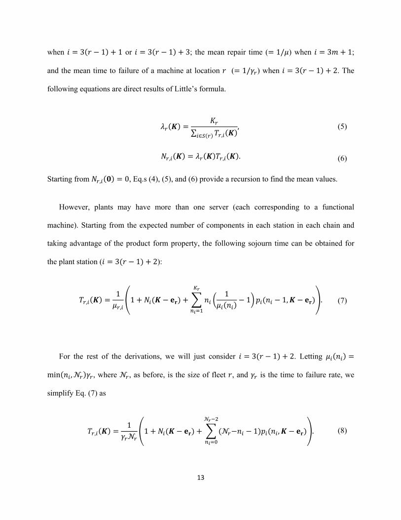
when 3 1 1 or 3 1 3; the mean repair time ( 1/ ) when 3 1;
and the mean time to failure of a machine at location ( 1/ ) when 3 1 2. The
following equations are direct results of Little’s formula.
∑ ,
, (5)
, , .
(6)
Starting from , 0, Eq.s (4), (5), and (6) provide a recursion to find the mean values.
However, plants may have more than one server (each corresponding to a functional
machine). Starting from the expected number of components in each station in each chain and
taking advantage of the product form property, the following sojourn time can be obtained for
the plant station ( 3 1 2):
,1
,1
11 1, . (7)
For the rest of the derivations, we will just consider 3 1 2. Letting
min , , where , as before, is the size of fleet , and is the time to failure rate, we
simplify Eq. (7) as
,1
1 1 , . (8)
14
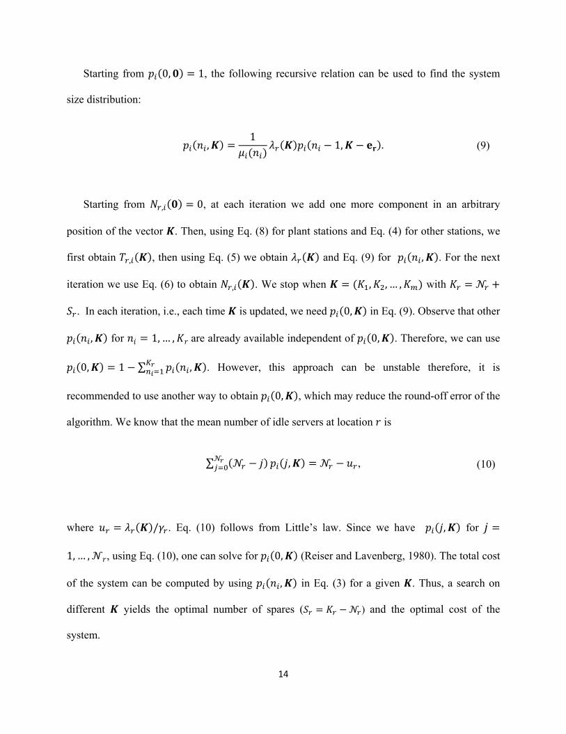
Starting from 0, 1, the following recursive relation can be used to find the system
size distribution:
,1
1, . (9)
Starting from , 0, at each iteration we add one more component in an arbitrary
position of the vector . Then, using Eq. (8) for plant stations and Eq. (4) for other stations, we
first obtain , , then using Eq. (5) we obtain and Eq. (9) for , . For the next
iteration we use Eq. (6) to obtain , . We stop when , , … , with
. In each iteration, i.e., each time is updated, we need 0, in Eq. (9). Observe that other
, for 1, … , are already available independent of 0, . Therefore, we can use
0, 1 ∑ , . However, this approach can be unstable therefore, it is
recommended to use another way to obtain 0, , which may reduce the round-off error of the
algorithm. We know that the mean number of idle servers at location is
∑ , , (10)
where / . Eq. (10) follows from Little’s law. Since we have , for
1, … , , using Eq. (10), one can solve for 0, (Reiser and Lavenberg, 1980). The total cost
of the system can be computed by using , in Eq. (3) for a given . Thus, a search on
different yields the optimal number of spares ( ) and the optimal cost of the
system.

15
V. Numerical Examples
Our goal in this section is to use the algorithm we have developed in Section 4 to compare
the performance of the DF and BC systems when transportation costs and times are significant.
Our second goal is to show via an example how this algorithm can be used to find the optimal
location for the centralized repair shop facility.
We start with a BC system having three locations. Each location has its own local repair
shop; therefore, they do not incur any transportation costs and the transportation time is
negligible (Figure 3). In addition to the parameters shown in Figure 3 where is the failure rate
of a component, we assume that each repair shop has the service rate of 10. Considering
1 and 10 for each location, the optimal number of spares ( ) is found to be
6 for each fleet as shown in Table 1 with the corresponding optimal costs. So the total system
cost is 3 6.14 18.42.
Figure 3: Three separate locations
Next, we assume that these three repair shops are merged into one making it a DF system.
Such a situation can arise if these fleets outsource their repair services to a third company or if
100.8
10 0.8
100.8

16
they would like to exploit the higher capacity of a centralized repair shop. As discussed by Yu,
Benjaafar, and Gerchak (2009), we set the repair rate of the central repair shop to 30, which
is the sum of individual repair rates of the BC system presented in Figure 3. In this case, we set
the location of the centralized repair shop at location 1, therefore, fleet 1 still has no
transportation delays or cost whereas fleets 2 and 3 need to send their broken components to the
central repair shop resulting in transportation costs and delay. We set the unit time transportation
costs to 0, 0.01, and mean transportation times to and from the repair shop for
fleet 2 and fleet 3 to 1/ 1/ 0.01. Table 2 shows the optimal number of spares and
corresponding costs in the DF system.
Table 1: Optimal solution for the BC system in Figure 3
Optimal Cost Total Holding Shortage Transportation
6 6.140 3.384 2.756 0
Table 2: Optimal solution for the DF system
Fleet Optimal Cost Total Holding Shortage Transportation
1 3 3.252 2.003 1.248 0 2 3 3.485 1.871 1.456 0.157 3 3 3.485 1.871 1.456 0.157
Total 9 10.223 5.747 4.160 0.315

17
Comparing the results in Tables 1 and 2, we see that the DF system has a total of 9 spare
parts for all fleets whereas the BC system allocates 18 in total. Not only the number of optimal
number of spares but also the optimal system cost decreases from 3 6.14 18.42 (for the BC
system) to 10.22 (for the DF system). Therefore, in this example we conclude that pooling the
repair shop capacity is beneficial.
However, this is not always the case. In Figure 4, we vary the unit time transportation costs
and (with ) on the x-axis while keeping all other parameters the same and observe
how the optimal system cost and the sum of optimal number of spares change. Figure 4 shows
that the sum of the optimal number of spares is not sensitive to transportation costs and remains
at 9. However, for 0.3, having a centralized repair shop at location 1 is no longer
beneficial since the optimal system cost of the DF system exceeds 18.42. This observation raises
the question of choosing the location of the repair shop correctly.
Figure 4: Optimal solution for
0
1
2
3
4
5
6
7
8
9
10
0
5
10
15
20
25
30
35
40
45
0 0.1 0.2 0.3 0.4 0.5 0.6 0.7 0.8 0.9 1
Num
ber of sparesTo
tal System Cost ($)
Transportation cost rates for locations 2 and 3
Total Cost Spare Parts

18
We now take advantage of our model to find the best location for the central repair shop. In
the above mentioned example, assume that locations 2 and 3 are close to each other so that it
costs 0.1 per unit time to transport one component between locations 3 to 2, whereas
transportation cost rates from either location 2 or 3 to location 1 is 0.3. Figure 4 shows that if the
centralized repair shop is kept at location 1, the optimal cost of the DF system is 19.36 when
0, 0.3, which exceeds 18.42. This makes repair shop pooling unbeneficial.
However, if we move the central repair shop to location 2, then transportation cost rates change
to 0.3, 0, and 0.1. The optimal cost of this system is 16.22, which means the
pooling of repair shop is beneficial provided that the central repair shop resides at location 2.
Figure 5: Effect of transportation rate 100 .
Next, we revisit the case where repair shop is hosted at location 1. With fixed transportation
cost rates for fleets 2 and 3 as c c 0.2 and 100, we reduce the transportation rate of
fleet 2 (reciprocal of the mean transportation time) from 100 to 0.5 (Figure 5). Observe that
from 100 to 30, the optimal number of spares remains the same and the total cost is almost fixed
0
5
10
15
20
25
30
35
40
45
50
0
5
10
15
20
25
100 90 80 70 60 50 40 30 20 10 9 8 7 6 5 4 3 2 1 0.9 0.8 0.7 0.6 0.5
Num
ber of SparesTo
tal System Cost ($)
Transportation rates of location 2
Total Cost Spare parts at location 2
19
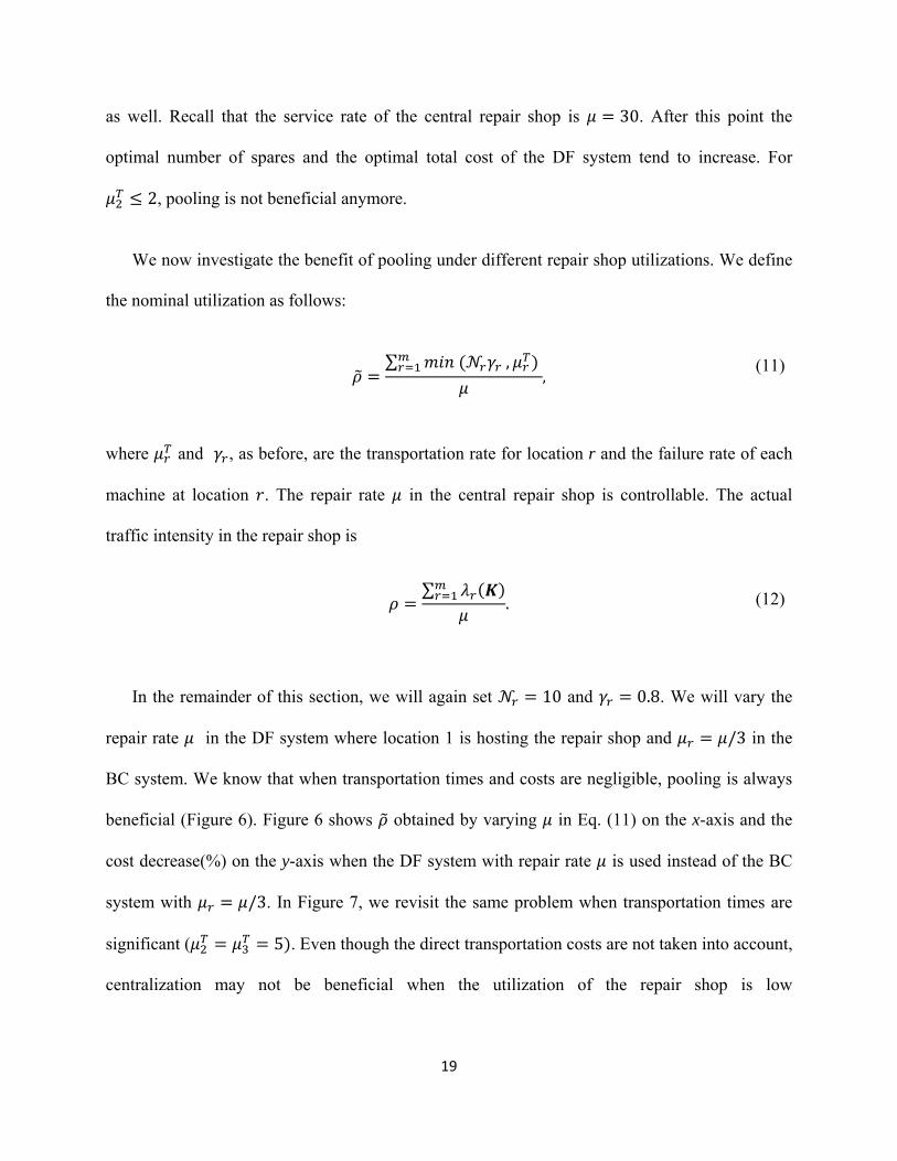
as well. Recall that the service rate of the central repair shop is 30. After this point the
optimal number of spares and the optimal total cost of the DF system tend to increase. For
2, pooling is not beneficial anymore.
We now investigate the benefit of pooling under different repair shop utilizations. We define
the nominal utilization as follows:
∑ ,
, (11)
where and , as before, are the transportation rate for location r and the failure rate of each
machine at location . The repair rate in the central repair shop is controllable. The actual
traffic intensity in the repair shop is
∑
. (12)
In the remainder of this section, we will again set 10 and 0.8. We will vary the
repair rate in the DF system where location 1 is hosting the repair shop and /3 in the
BC system. We know that when transportation times and costs are negligible, pooling is always
beneficial (Figure 6). Figure 6 shows obtained by varying in Eq. (11) on the x-axis and the
cost decrease(%) on the y-axis when the DF system with repair rate is used instead of the BC
system with /3. In Figure 7, we revisit the same problem when transportation times are
significant ( 5 . Even though the direct transportation costs are not taken into account,
centralization may not be beneficial when the utilization of the repair shop is low

20
Figure 6: Cost saving by pooling the repair shops ( 0, 0
Figure 7: Cost saving by pooling the repair shops ( 0, 5
Figure 8: Cost saving by pooling the repair shops ( 0.1, 5
Figure 9: Cost saving by pooling the repair shops ( 0.1, 20
Figure 10: Cost saving by pooling the repair shops ( 0.01, 100
(negative y-values indicate a cost increase in the DF system). Furthermore, considering
transportation costs decreases the benefit of pooling even more (Figure 8). In this case, the
threshold utilization after which pooling is beneficial is higher. However, transportation rates of
5 in comparison to the failure rates 0.8 might appear to be low. Keeping the
0%
10%
20%
30%
40%
50%
60%
0.40
0.42
0.44
0.47
0.50
0.53
0.57
0.62
0.67
0.73
0.80
0.89
1.00
cost decrease (%
)
‐30%
‐20%
‐10%
0%
10%
20%
30%
40%
0.40
0.42
0.44
0.47
0.50
0.53
0.57
0.62
0.67
0.73
0.80
0.89
1.00
cost decrease (%
)
‐70%‐60%‐50%‐40%‐30%‐20%‐10%0%10%20%30%
0.40
0.42
0.44
0.47
0.50
0.53
0.57
0.62
0.67
0.73
0.80
0.89
1.00
cost decrease (%
)
‐30%
‐20%
‐10%
0%
10%
20%
30%
40%
0.40
0.42
0.44
0.47
0.50
0.53
0.57
0.62
0.67
0.73
0.80
0.89
1.00
cost decrease (%
)
0%
10%
20%
30%
40%
50%
0.40
0.42
0.44
0.47
0.50
0.53
0.57
0.62
0.67
0.73
0.80
0.89
1.00
cost decrease (%
)

21
transportation costs fixed ( 0.1 , Figure 9 shows the cost reduction when transportation
rates are 20. The last Figure 10 shows that when transportation times and costs are
small and negligible, we have a similar situation as presented in Figure 6 and centralization of
the repair shops is beneficial.
VI. Conclusion and Future Work
In this paper, we consider a system of fleets of machines subject to failure due to a critical
repairable component. To minimize the down time costs, the system carries spare parts
inventories. When the transportation times and costs are negligible, repair shop pooling is
beneficial. For the problems in which the transportation times and costs are not negligible, we
have developed a model for a system with a centralized repair shop operating under the FCFS
dispatching policy and local spare parts inventories at each location. Using this model, we show
that repair shop pooling is not beneficial is some cases. We also use our model to find the best
location for the central repair shop to minimize overall system costs. In the future, a hybrid of
local and central repair shops can be analyzed. In this hybrid system, a fraction of broken
components with minor problems may be repaired locally and go back to service shortly. The
other more severe failed components with major problem are sent to the central repair shop.
Moreover, variable repair rates depending on the number of components waiting for service in
the repair shop can be incorporated in the model.
References
Altiok, T. 1997. Performance analysis of manufacturing systems. Springer Verlag.
Benjaafar, S., W. L. Cooper, and J. S. Kim. 2005. On the benefits of pooling in production-inventory systems. Management Science 51, (4): 548-65.

22
Breuer, L., Baum, D. (2005). An introduction to queueing theory and matrix-analytic methods. Kluwer Academic Publishers.
Buzen, J. P. 1973. Computational algorithms for closed queueing networks with exponential servers. ACM 16. (9): 527-31.
Eppen, G. D. 1979. Effects of centralization on expected costs in a multi-location newsboy problem. Management Science 25, (5): 498-501.
Gerchak, Y., and Q. M. He. 2003. On the relation between the benefits of risk pooling and the variability of demand. IIE Transactions (Institute of Industrial Engineers) 35, (11): 1027-31.
Gordon, W. J., and G. F. Newell. 1967. Closed queuing systems with exponential servers. Operations Research 15, (2): 254-65.
Gross, D. and C. M. Harris. 1998. Fundamentals of Queueing Theory, John Wiley & Sons, New York.
Hui, E. Y. Y., and A. H. C. Tsang. 2004. Sourcing strategies of facilities management. Journal of Quality in Maintenance Engineering 10, (2): 85-92.
Kumar, R., and T. Markeset. 2007. Development of performance-based service strategies for the oil and gas industry: A case study. Journal of Business and Industrial Marketing 22, (4): 272-80.
Reiser, M., and S. S. Lavenberg. 1980. Mean-value analysis of closed multichain queuing networks. Journal of the ACM 27, (2): 313-22.
Sahba, P., B. Balcıoğlu, and D. Banjevic. 2010. Dispatching policies for a spare parts provisioning problem. Under Review.
Yu, Y., S. Benjaafar, and Y. Gerchak. 2008. Capacity pooling and cost sharing among independent firms in the presence of congestion. Under Review.