A Model-Based Residual Approach

for Human-Robot Collaboration

during Manual Polishing Operations I

Claudio Gaza, Emanuele Magrinia, Alessandro De Luca∗,a

aDipartimento di Ingegneria Informatica, Automatica e Gestionale,Sapienza Universita di Roma, Via Ariosto 25, 00185 Roma, Italy

Abstract

A fully robotized polishing of metallic surfaces may be insufficient in case of parts

with complex geometric shapes, where a manual intervention is still preferable.

Within the EU SYMPLEXITY project, we are considering tasks where manual

polishing operations are performed in strict physical Human-Robot Collabora-

tion (HRC) between a robot holding the part and a human operator equipped

with an abrasive tool. During the polishing task, the robot should firmly keep

the workpiece in a prescribed sequence of poses, by monitoring and resisting to

the external forces applied by the operator. However, the user may also wish to

change the orientation of the part mounted on the robot, simply by pushing or

pulling the robot body and changing thus its configuration. We propose a con-

trol algorithm that is able to distinguish the external torques acting at the robot

joints in two components, one due to the polishing forces being applied at the

end-effector level, the other due to the intentional physical interaction engaged

by the human. The latter component is used to reconfigure the manipulator

arm and, accordingly, its end-effector orientation. The workpiece position is

kept instead fixed, by exploiting the intrinsic redundancy of this subtask. The

controller uses a F/T sensor mounted at the robot wrist, together with our re-

IThis work is partly supported by the European Commission, within the H2020-FoF-2014637080 SYMPLEXITY project (www.symplexity.eu).

∗Corresponding authorEmail addresses: gaz@diag.uniroma1.it (Claudio Gaz), magrini@diag.uniroma1.it

(Emanuele Magrini), deluca@diag.uniroma1.it (Alessandro De Luca)

Preprint submitted to Mechatronics February 8, 2018

cently developed model-based technique (the residual method) that is able to

estimate online the joint torques due to contact forces/torques applied at any

place along the robot structure. In order to obtain a reliable residual, which

is necessary to implement the control algorithm, an accurate robot dynamic

model (including also friction effects at the joints and drive gains) needs to be

identified first. The complete dynamic identification and the proposed control

method for the human-robot collaborative polishing task are illustrated on a 6R

UR10 lightweight manipulator mounting an ATI 6D sensor.

Key words: physical HRI, human-robot collaboration, robot control, robot

dynamic modeling, friction identification, contact force estimation, abrasive

polishing

1. Introduction

One challenging objective in the next generation of smart factory floors is to

bring humans and robots close together, working efficiently and collaborating

safely in the same shared manufacturing environment. This is being pursued

in several national and international industry-oriented programs under different5

names, such as Industry 4.0, Cyber-Physical Systems, or Internet of Things [1].

In this context, recent research progresses dealing with physical Human-

Robot Interaction (pHRI) have covered mechanical, actuation, sensing, plan-

ning, and control issues in an integrated way, with the goal of increasing safety

and dependability of robotic systems [2]. In [3], we have originally proposed a10

control architecture devoted to pHRI, which is organized in three nested func-

tional layers addressing, respectively, human-robot safety, coexistence, and col-

laboration.

Safety is the inherent and most important feature of a robot that has to

work close to or collaborate with human beings. Due to the limits of sensors15

and robot motion capabilities, e.g., when the human moves faster than the

robot can sense or counteract, undesired contacts or collisions with humans may

occur. This is handled in the lowest (direct) layer of the control architecture,

2

which implements sensorless collision detection, isolation, and reflex reaction

based on our residual method [4, 5, 6], a model-based scheme that monitors the20

generalized momentum of the robot.

By coexistence, we mean the robot capability of sharing a dynamic environ-

ment with humans, without requiring mutual contact or coordination of actions.

The intermediate layer in our architecture realizes coexistence by featuring on-

line collision avoidance capabilities, based on workspace monitoring by external25

sensors such as cameras or RGB-Depth devices (see, e.g., [7, 8]), while human

safety requirements are still being imposed.

Finally, the top control layer addresses collaboration, in which the robot

performs a complex task with direct human interaction and coordination. We

refer to safe collaboration when this activity does not rule out a safe robot30

behavior, namely when both safety and coexistence features are guaranteed

during the collaboration phase.

As a result, upper layers in this architecture will prescribe only robot reactive

behaviors that are consistent with the objectives and constraints of lower layers.

Interestingly enough, the three layers of the proposed control architecture can35

be easily mapped to the most recent requirements of safety standards and rec-

ommendations for collaborative robots, such as the ISO technical specification

TS-15066 [9, 10].

The top control layer handles both contact-less human-robot coordination

and, most importantly here, physical collaboration tasks, in which a continuous40

and intentional contact takes place with a controlled exchange of forces/torques,

as activated by multimodal communication such as voice, gestures, or touch [11,

12].

In common industrial applications, the robot interacts with the environment

mainly with a tool mounted on the end-effector. A force/torque (F/T) sensor45

placed on the final robot flange provides then the exchanged forces/torques.

When the contact point is known in advance, the problem of sensor-less contact

force estimation without the use of a F/T sensor has been addressed in [13],

based on motor torque/current measurements. A dithering feedforward torque

3

is used to decrease uncertainties due to friction, so as to improve force esti-50

mation when the robot is not in motion. Under similar operative conditions,

learning-based approaches have also been applied for estimating exchanged ex-

ternal forces [14, 15]. The estimated external force and the saturation of motor

control torques can be used to keep the actual exchanged forces under a safety

threshold [16].55

In order to execute a wider range of activities involving Human-Robot Col-

laboration (HRC), physical contacts should not be limited in advance to a des-

ignated tool at the end-effector level, but rather whole-arm manipulation condi-

tions should be considered. This raises the additional issue of reconstructing the

exchanged forces at generic contact points along the robot structure, either by60

measuring them (e.g., using tactile sensitive skin in different locations [17]) or by

estimating them in an indirect way, possibly combining model-based methods

with other less invasive external sensors.

In [18], a first example of a method that estimates contact forces occurring

at generic points (a priori unknown) on the robot arm was given. This was65

obtained by a so-called virtual force sensing approach, combining proprioceptive

information of the residual method with localization of the contact location

provided by a Kinect camera. The framework has been enriched in successive

works [19, 20], where other generalized control laws have been developed thanks

to the improved knowledge of the dynamic model obtained on the KUKA LWR70

4+ robot [21, 22], which is exploited for the computation of the residual.

The H2020 European research project SYMPLEXITY [23] aims at devel-

oping solutions for complex surface finishing operations to be accomplished by

collaborative work of humans and robots. Within this project, we are currently

transferring our know-how on physical human-robot interaction to industrial75

set-ups proposed by end users.

In this paper, we present the core control algorithm that allows a human op-

erator to kinesthetically reorient a workpiece held by the robot. In this context,

the user should be able to change the orientation of the part while performing

a surface polishing operation on it. It is desirable to achieve this in a natural80

4

way, by manually pushing or pulling the robot structure, rather than by com-

manding the robot via a separated interface (such as a teach-pendant, a pedal,

or a keyboard). To this purpose, we need to decouple the effects of the two

types of contact forces exerted by the operator against the robot: one due to

the execution of the manual polishing task on the workpiece mounted on the85

robot end effector, the other due to the intentional reconfiguration force applied

to the robot body. While the polishing force can be directly measured thanks

to a F/T sensor mounted on the end-effector, the residual signals can estimate

the torques at robot joint level resulting from both types of contact forces. By a

suitable but simple elaboration, the intentional component can be isolated and90

will be used by the controller to command the robot motion. In particular, the

control law exploits the redundancy of the robot by specifying joint velocities

in the null-space of an appropriate kinematic task, keeping the position of the

end-effector fixed, while allowing relaxation of its orientation.

The paper is organized as follows. Section 2 briefly introduces the SYM-95

PLEXITY laser polishing cell in which a HRC task has to be accomplished in

a manual station. Section 3 presents the proposed control algorithm to achieve

the HRC task. For the robot used in the experiments, a Universal Robots UR10,

Section 4 presents the complete identification of the dynamic model, which is

needed for the computation of residuals —the core signals in our model-based100

solution approach. This dynamic model is improved in accuracy with respect

to the one supplied by the manufacturer, and includes also the novel estima-

tion of friction terms and current-to-torque motor gains. Section 5 reports on

the obtained experimental results, illustrated also in a video accompanying the

paper. Finally, conclusions and on-going work are summarized in Sec. 6.105

2. Human-robot collaboration in a manual polishing station

Three main technologies are used for the robotized smoothing of metallic sur-

faces down to micrometer levels of roughness: Abrasive Finishing (AF), Laser

Polishing (LP), and Fluid-jet Polishing (FP). All three technologies have been

5

Kinect 1

Kinect 2

LP Machine

Airlock

Ultrasonic Bath Measurement Tool

Operator

UR10 Robot HRC Desk

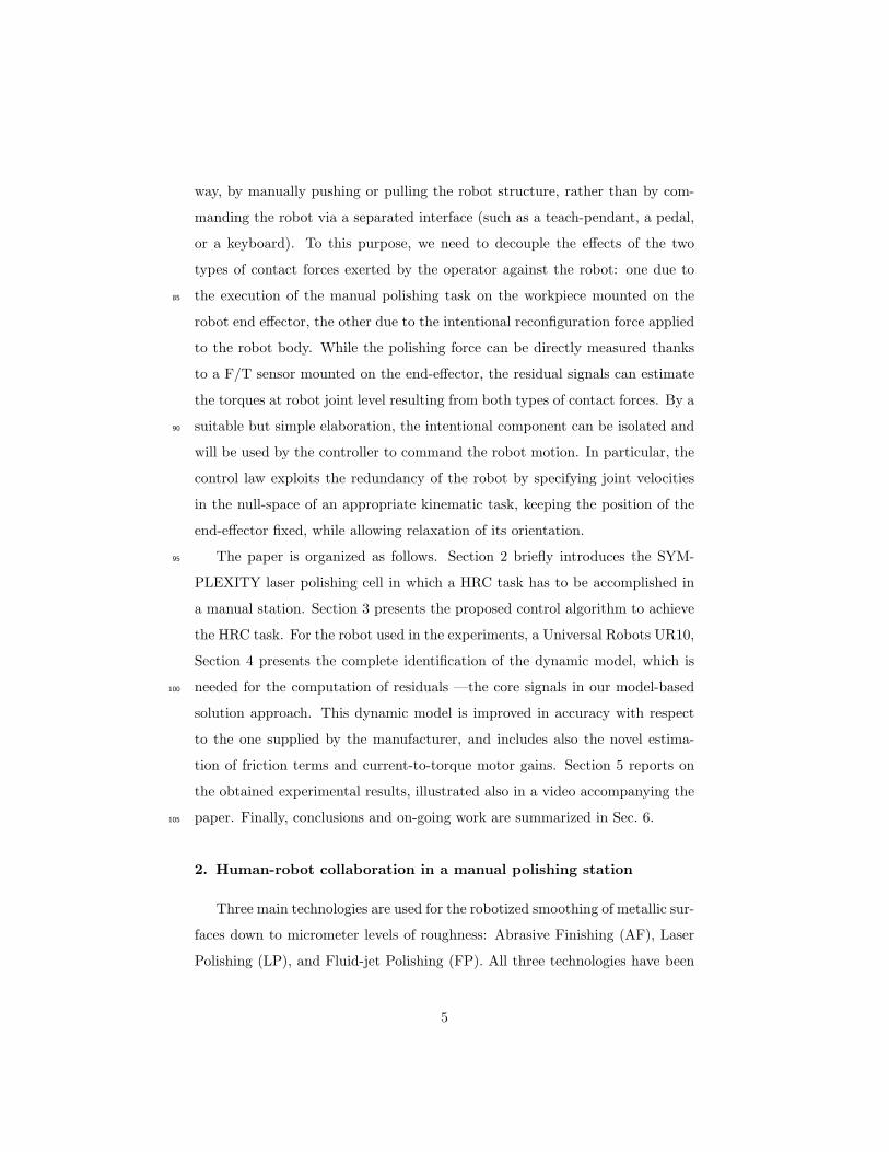
Figure 1: Layout of the manual polishing station in the SYMPLEXITY LP cell (in V-

REP [24]).

considered in industrial case studies within the SYMPLEXITY project, espe-110

cially from the point of view of robot collaboration with a human operator both

in execution and learning. We focus here on the LP cell. The safety require-

ments in this case do not allow a human to interfere at any time with the laser

source, which is used with a robot moving inside a closed machine. However,

this fast and precise technology for surface finishing can be used only if the115

roughness state of the workpiece at the start is already acceptable. In order

to check this, metrology should be used to assess the initial quality of the part

and, in case, manual abrasive polishing should be performed on selected parts.

In this situation, HRC represents a handy solution.

A virtual rendering of the various components of the LP cell is shown in120

Fig. 1. Access to the LP machine occurs through an automatic airlock. A robot

is used to move around the workpiece, from the operator desk to the ultrasonic

cleaning bath, or from the measurement tool to the airlock, and so on. When

the part is in need of a manual polishing before being ready to be processed by

the LP machine, it will be carried by the robot in front of the human operator.125

6

HRC will occur then, with the human using a tool to polish selected surfaces

of the part (those indicated graphically on a Human-Machine Interface) and

the robot holding the workpiece in a specified sequence of poses. The correct

and safe operation of the manual polishing station will be monitored by two

RGB-D (Kinect) sensors, measuring in real time minimum distances between130

selected control points on the robot and the whole environment (including the

dynamically moving human operator) [8]. This will prevent accidental collisions

and avoid unintended contacts when the robot is moving around (safe coexis-

tence). On the other hand, an obvious exchange of forces should occur at the

end-effector level during execution of the manual polishing, with forces in the135

order of 20 N and peaks up to 35 N. In addition, extra intentional forces will be

applied by the human operator to the robot body to reorient the end-effector

and complete the task in a ergonomic and natural way. Operation and control

of these physical HRC events is presented in the next section.

The cell will be used for polishing small bio-compatible metallic parts of140

complex shape for physiological uses in medicine. The weight of the parts is in

the order of 10 grams —negligible with respect to the part holder and gripper

mounted on the robot end-effector.

3. Decoupling the external forces when a robot holds a workpiece

Consider a rigid robot manipulator with n joints and generalized coordinates

q ∈ Rn, modeled by Euler-Lagrange equations in the usual form

M(q)q +C(q, q)q + g(q) + τf (q) = τ + τ ext, (1)

where M(q) is the positive definite, symmetric robot inertia matrix, Coriolis145

and centrifugal forces (quadratic in q) are factorized using a square matrix

C(q, q) such that M−2C is skew-symmetric, g(q) are the gravity terms, τf (q)

contains frictional forces, τ are the motor torques at the joints, and τ ext ∈ Rn

is the vector of joint torques resulting from possible external Cartesian forces.

When the robot is holding a workpiece to be manually polished, the forces150

and moments that the human operator exerts on the surface of the part are

7

reflected along the robot structure from the end-effector to the robot joints. In

some cases, these generalized forces could even move the joints, if brakes were

not activated or high-gain positional feedback was not used on the motors1.

This situation has to be avoided in order not to compromise the quality of the155

operation carried out on the part. Nevertheless, it may be desirable, or even

necessary, during such an operation to reorient the workpiece in order to achieve

better results. When the robot is firmly holding an object, though, exerting a

force on the workpiece would produce no motion. Conversely, intentional forces

exerted by the operator on the manipulator structure could usefully affect the160

reorientation of the part. Thus, such a contact situation should be detected, the

original control task should be relaxed accordingly, and a new suitable command

generated, by exploiting the degrees of kinematic redundancy that the robot

gains from the relaxation of the original task. On the other hand, contacts

occurring occasionally on the manipulator body when the robot is in motion165

should always be considered as accidental collisions and handled differently for

safety (see, e.g., [6]).

The forces exerted on the workpiece at the end-effector and on the manip-

ulator structure are both reflected at the joint level as τ ext in eq. (1). In view

of the above discussion, it is however necessary to separate these two contribu-

tions, in such a way that only the intentional force acting on the robot links is

fed into the robot motion control law. Let

τ ext = τ e + τ c = JTe (q)F e + JTc (q)F c, (2)

with vectors τ e ∈ Rn and τ c ∈ Rn being, respectively, the joint torque due to the

generalized force F e =(fTe m

Te

)T∈ R6 exerted on the end-effector, and the

joint torque due to the generalized force at the contact F c =(fTc m

Tc

)T∈ R6.170

Moreover, Je ∈ R6×n and Jc ∈ R6×n are, respectively, the (geometric) Jacobian

1High-gain positional feedback is preferred over braking, in order not to interrupt the

operation flow for too long, as well as to transit between successive phases in a smoother way

(i.e., by control).

8

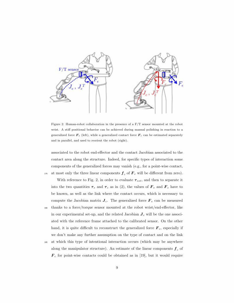
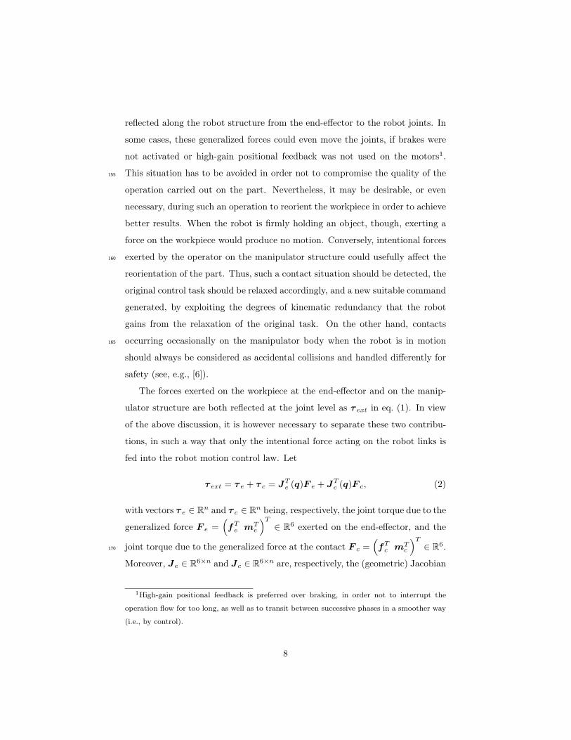
Fe

Je , JeT

F/T sensor

Fc Fe

Jc , JcT

Figure 2: Human-robot collaboration in the presence of a F/T sensor mounted at the robot

wrist. A stiff positional behavior can be achieved during manual polishing in reaction to a

generalized force F e (left), while a generalized contact force F c can be estimated separately

and in parallel, and used to reorient the robot (right).

associated to the robot end-effector and the contact Jacobian associated to the

contact area along the structure. Indeed, for specific types of interaction some

components of the generalized forces may vanish (e.g., for a point-wise contact,

at most only the three linear components f c of F c will be different from zero).175

With reference to Fig. 2, in order to evaluate τ ext, and then to separate it

into the two quantities τ e and τ c as in (2), the values of F e and F c have to

be known, as well as the link where the contact occurs, which is necessary to

compute the Jacobian matrix Jc. The generalized force F e can be measured

thanks to a force/torque sensor mounted at the robot wrist/end-effector, like180

in our experimental set-up, and the related Jacobian Je will be the one associ-

ated with the reference frame attached to the calibrated sensor. On the other

hand, it is quite difficult to reconstruct the generalized force F c, especially if

we don’t make any further assumption on the type of contact and on the link

at which this type of intentional interaction occurs (which may be anywhere185

along the manipulator structure). An estimate of the linear components f c of

F c for point-wise contacts could be obtained as in [19], but it would require

9

the identification of the actual contact position on the link (and thus of Jc), by

means of an external sensor, like a depth camera.

However, the solution is relatively easy when a F/T wrist sensor is avail-

able. In fact, for our purposes we only need to obtain an estimate of the τ c

component, and not of its original source F c and location. Since τ e can be

obtained from the F/T sensor measurement, it is sufficient to resort to a slight

modification of the model-based approach originally proposed in [5] for sensor-

less collision detection, which generates a residual vector r ∈ Rn by monitoring

the generalized momentum p = M(q)q of the robot. Thus, we can define a

modified (and computable) residual as

r(t) = G

(M(q)q −

∫ t

0

(CT (q, q)q − g(q)− τf (q) + τ + τ e + r

)ds

), (3)

where G ∈ Rn×n is a positive, diagonal gain matrix, and we set r(0) = 0 when190

the robot initially at rest. All terms in (3) can be evaluated efficiently, once a

reliable robot dynamic model (1) is available. Note in particular that:

• no joint acceleration measurements nor inversion of the inertia matrix are

needed in the residual formula;

• the joint torque contribution τ e of the generalized force acting on the195

robot end-effector (due to the manual polishing) is subtracted from the

residual —a component which was absent in [5];

• the applied command torques τ , which are not restricted to any specific

control law, are obtained from the measured motor currents i, as τ = Ki,

with K = diag{K1, . . . ,Kn} and where Kj > 0 is the current-to-torque200

gain of the jth motor;

• the friction term τf (q) is indeed critical, being usually the most difficult

to be modeled and correctly identified;

• at very low robot speed (and at rest), the residual can be simplified by

eliminating all terms that vanish together with the joint velocity q, leaving205

essentially the gravity torque g(q), the joint torques τ and τ e, and the

static friction part of the torque τf , if any;

10

• residuals have the same dimensional units [Nm] of motor torques at the

joints; they can also be evaluated at the level of motor currents (in [A]

units), scaling each term by the relative gain Kj .210

Using the properties of the Christoffel symbols [28] for the conservative ve-

locity terms in the dynamic model (1), it is easy to check that the residual vector

r will automatically satisfy the following relation, which is useful for analysis:

r = G (τ c − r) , or, equivalently, ri = Gi(τc,i − ri), i = 1, . . . , n. (4)

Therefore, the residual r will stay at zero (up to noise and model uncertain-

ties) as long as there is no external joint torque applied along the manipulator

structure. Once τ c is present, the residual will react to it as a first-order stable

linear filter. As a result, r will converge exponentially to the true value of τ c, if

this is constant at least for a short period of time. The residuals will also return215

exponentially to zero when the contact is removed —an interesting feature for

our application. In general, we will use sufficiently large gains Gi’s and, based

on (4), consider in our application the residual r and the joint torque τ c as

superposed, i.e., r ' τ c. An example of behavior of residuals in practice is

reported in Sec. 4.5, for a UR10 robot having n = 6 (see Fig. 10).220

The control concept at the basis of this work is to produce self-motions of

the robot in response to the human operator pushing by hand the manipulator

structure, generating thus a τ c that is estimated by r. The target is to keep

the position of the end-effector fixed while relaxing its orientation. This will

allow the operator to easily reorient the part to be manually polished, without

pushing a button, touching a screen, or using other separate HMI devices, and

eventually not even needing to suspend the manual polishing task as we shall

see. To this purpose, we rewrite the Jacobian Je(q) into its linear and angular

components as

Je(q) =

Jp(q)

Jo(q)

, Jp ∈ R3×n, Jo ∈ R3×n.

Assuming that the robot joints are controlled by velocity references (kinematic

control), in order to provide the proper self-motion, the following control law is

11

adopted

q = J#p (q)Kp

(pd − p(q)

)+(I − J#

p (q)Jp(q))Krr, (5)

where the n × 3 matrix J#p is the unique pseudoinverse of the linear Jacobian

Jp, pd ∈ R3 is the desired (constant) position of the end-effector, p ∈ R3 is

its actual position, as computed through the robot direct kinematics, and Kp

and Kr are (diagonal) gain matrices of dimension 3× 3 and n×n, respectively.

In (5), the residual r will drive the null-space joint velocities through the n× n225

projection matrix I − J#p Jp of the positional task. Since an equivalent joint

torque generates a joint velocity command, the controller (5) belongs to the

class of admittance laws at the joint level. The Cartesian gains Kp will be

chosen as large as possible in order to realize a very stiff position control. Note

finally that the choice of a kinematic control law, as opposed to a torque control230

law for τ , is mandatory when the robot has a closed control architecture and no

direct access to motor currents/torques is allowed (as in the case of the UR10

manipulator).

4. Dynamic modeling and identification of the UR10 manipulator

4.1. Motivation235

As target robot for our HRC control task, we have considered the 6-dof

lightweight manipulator UR10 by Universal Robots. Figure 3 shows the kine-

matic frames and the associated table of Denavit-Hartenberg (DH) parameters.

Summarizing the result of Sec. 3, a good knowledge of the dynamic model of

the robot is mandatory in order to have a reliable residual signal (3), necessary240

to implement the control action (5). The manufacturer distributes a software

simulator on its website [25], which includes data files with the numerical values

of all dynamic parameters of the UR10 manipulator. We exploited those data

in order to reconstruct all dynamic terms in the model (1) of this robot.

Unfortunately, we found that the dynamic model reconstructed in this way245

is not sufficiently reliable, both in static and dynamic conditions. Extensive

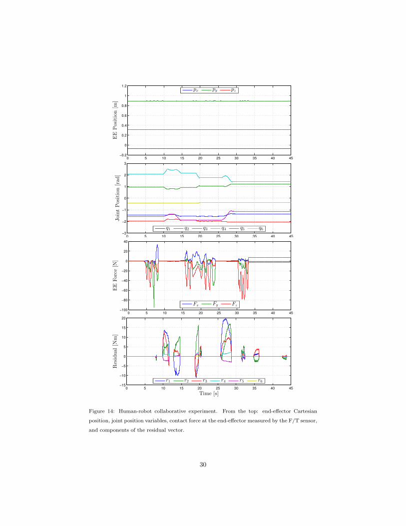
12

y0

z0

z1

z2

y1

x2

z3

x3 z4

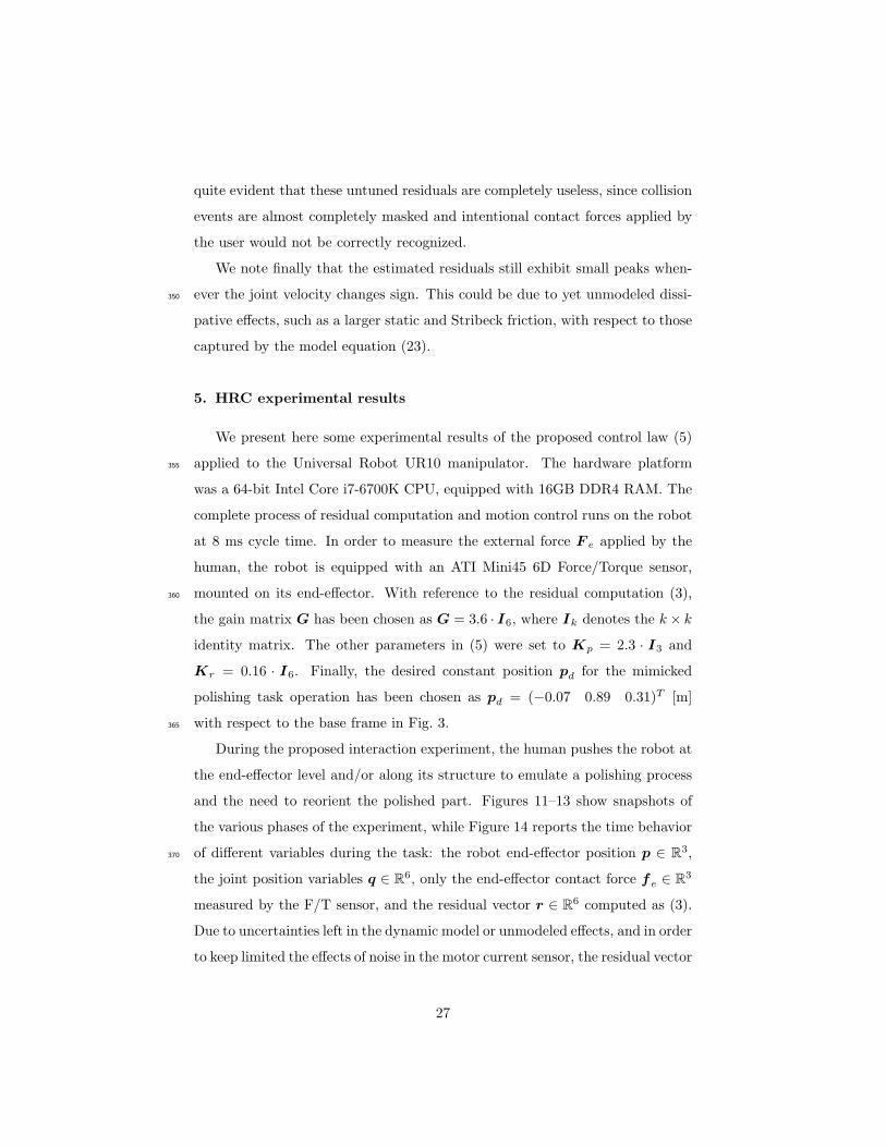
y4

z5

y5

z6

y6

x1

x0

x6 x5

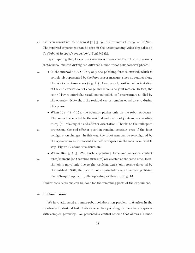
x4

92.2 163.9

115.

7 57

1.6

612.

7 12

8

i ai αi di θi

1 0 −π/2 d1 = 128 q1

2 a2 = 612.7 0 0 q2

3 a3 = 571.6 0 0 q3

4 0 −π/2 d4 = 163.9 q4

5 0 π/2 d5 = 115.7 q5

6 0 0 d6 = 92.2 q6

Figure 3: The UR10 manipulator with the chosen (classical) DH frames and the associated

table of kinematic parameters. Lengths are expressed in [mm].

comparisons between measured motor currents2 and currents computed via the

nominal data provided by the manufacturer on a (relatively slow) sinusoidal

motion trajectory showed quite different behaviors on all joints, with deviations

as large as 9 [A] for the second joint. These differences are due in part also to the250

friction term τf , whose parameters are in fact not provided by the manufacturer.

Even in static conditions, we found differences in the evaluation of the currents

associated with the gravity term g(q).

As a result, when used within the residual (3), the dynamic data of the robot

manufacturer would lead to a poor discrimination of contacts, e.g., with multiple255

false positives or false negatives (depending on the thresholds of detection). This

motivated us to perform a new identification procedure in order to improve the

accuracy of the terms in the dynamic model.

2In all experiments, measurements of joint positions q and motor currents i were collected

using the URScript Programming Language [26].

13

4.2. Identification in the presence of unknown motor gains

We present here the basic identification procedure that is needed for the260

UR10 manipulator. The specific features of this robot are the unknown current-

to-torque motor gains (aka, drive gains), the presence of a relatively large friction

component, and the availability of joint position and motor current measure-

ments only (no joint torque sensor). This combination calls for some adapta-

tion of otherwise standard robot dynamic identification methods (see, e.g., [27]).265

From now on, we set specifically n = 6 in (1).

Given the linear dependence of the dynamic model on the dynamic param-

eters of the robot links [28], it is possible to rearrange the left-hand side of (1)

in terms of a full rank regressor matrix Y ∈ R6×p that multiplies a vector

π ∈ Rp of dynamic coefficients, i.e., a number p of linear combinations of the

link dynamic parameters [29], as

Y (q, q, q)π = τ = Ki. (6)

The vector τ ∈ R6 of motor torques is expressed as the product of the drive

gains matrix K = diag{K1, . . . ,K6} times the vector of motor currents i ∈ R6.

Since the drive gains are also unknown, we can formally divide each of the

six equations in (6) by the corresponding Kj , thus obtaining the new linear

equations

Y j(q, q, q)π(j) = ij , j = 1, . . . , 6, (7)

where Y j ∈ Rp is the jth row of the regressor Y , ij is the current of motor j,

and we have extended the vector π of dynamic coefficients, by replicating it in

a scaled form relative to each joint as

π(j) =(π1

Kj. . .

πpKj

)T∈ Rp, j = 1, . . . , 6. (8)

In matrix form, equations (7) and (8) are rewritten as

Y [e](q, q, q) π[e] = i, (9)

where the extended vector of dynamic coefficients π[e] ∈ R6p is

π[e] =(π(1)T

π(2)T

. . . π(6)T)T

14

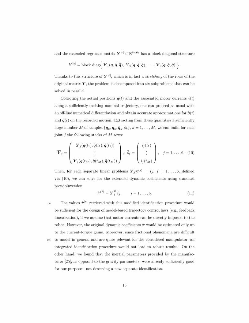
and the extended regressor matrix Y [e] ∈ R6×6p has a block diagonal structure

Y [e] = block diag{Y 1(q, q, q), Y 2(q, q, q), . . . ,Y 6(q, q, q)

}.

Thanks to this structure of Y [e], which is in fact a stretching of the rows of the

original matrix Y , the problem is decomposed into six subproblems that can be

solved in parallel.

Collecting the actual positions q(t) and the associated motor currents i(t)

along a sufficiently exciting nominal trajectory, one can proceed as usual with

an off-line numerical differentiation and obtain accurate approximations for q(t)

and q(t) on the recorded motion. Extracting from these quantities a sufficiently

large number M of samples {qk, qk, qk, ik}, k = 1, . . . ,M , we can build for each

joint j the following stacks of M rows:

Y j =

Y j(q(t1), q(t1), q(t1))

...

Y j(q(tM ), q(tM ), q(tM ))

, ij =

ij(t1)

...

ij(tM )

, j = 1, . . . , 6. (10)

Then, for each separate linear problems Y jπ(j) = ij , j = 1, . . . , 6, defined

via (10), we can solve for the extended dynamic coefficients using standard

pseudoinversion:

π(j) = Y#

j ij , j = 1, . . . , 6. (11)

The values π[e] retrieved with this modified identification procedure would270

be sufficient for the design of model-based trajectory control laws (e.g., feedback

linearization), if we assume that motor currents can be directly imposed to the

robot. However, the original dynamic coefficients π would be estimated only up

to the current-torque gains. Moreover, since frictional phenomena are difficult

to model in general and are quite relevant for the considered manipulator, an275

integrated identification procedure would not lead to robust results. On the

other hand, we found that the inertial parameters provided by the manufac-

turer [25], as opposed to the gravity parameters, were already sufficiently good

for our purposes, not deserving a new separate identification.

15

Therefore, we will pursue here a different, more structured two-step iden-280

tification approach. First, we estimate in static conditions both the dynamic

coefficients in the gravity vector g(q) and the drive gains K, by using two sets

of experiments with and without a known payload [22, 30]. Next, we use this

information to estimate the friction term τf (q) in dynamic conditions.

4.3. Estimating gravity coefficients and motor gains285

With reference to Fig. 3, we consider the UR10 manipulator mounted on

a horizontal table. The gravity acceleration is then γ =(

0 0 −g0)T

, with

g0 = 9.81 m/s2. In static conditions, q = q = 0, equations (6–9) specialize to

g(q) = col{gj(q)

}= Y g(q)πg = Ki

⇒ g[e](q) = col{gj(q)Kj

}= Y [e]

g (q)π[e]g = i.

(12)

The gravity vector g(q) ∈ R6 (in [Nm] units) is computed symbolically using

a Lagrangian approach, then linearly parametrized in terms of the dynamic

coefficients πg, and finally scaled in the form g[e](q) ∈ R6 (in [A] units) of

eq. (12). In this way, we found pg = dim πg = 10 independent coefficients.

However, because of the many structural zeros present in the different rows

Y g,j of Y g, the expanded vector π[e]g has only 30 non-vanishing components

(rather than 6 · pg = 60). Moreover, the drive gain K1 is not appearing in any

of these expressions, because the first component of the gravity vector g(q) is

16

g1 = 0 (the first joint axis is vertical). As a result, we have:

π[e]g =

ξ1/K2

...

ξ10/K2

ξ1/K3

...

ξ8/K3

ξ1/K4

...

ξ6/K4

ξ1/K5

...

ξ4/K5

ξ1/K6

ξ2/K6

∈R30, with

ξ1 = c6ym6

ξ2 = c6xm6

ξ3 = c5zm5 + c6zm6 + d6m6

ξ4 = c5xm5

ξ5 = c5ym5 + c4zm4 + d5m5

ξ6 = c4xm4

ξ7 = c3ym3

ξ8 = a3(m3 +m4 +m5 +m6) + c3xm3

ξ9 = c2ym2

ξ10 = a2(m2 +m3 +m4 +m5 +m6) + c2xm2.

(13)

The robot was moved to M = 500 different configurations spanning the

entire workspace, and motor currents were retrieved statically when each desired

position in the list was reached. Stacking these data, the extended gravity

coefficients in (13) were estimated, and the associated motor currents computed

as

π[e]g = Y

[e]

g

#

i ⇒ g[e](q) = Y [e]g (q) π[e]. (14)

In (14), i ∈ R6·500 is the stacked vector of measured motor currents, while

the numerical regressor Y[e]

g ∈ R6·500×30 is again block diagonal and has full

column rank. The obtained results are listed in Tab. 1, together with the values

computed using the manufacturer’s data for a comparison.

The estimation has been validated by placing the robot in 50 new joint290

configurations. The results are shown in Fig. 4. In all these static conditions,

the measured motor currents match now quite well with the estimated currents

g[e](q), whereas they are quite different from the currents computed from the

17

Dynamic coefficients Using UR10 nominal parameters Our estimation

ξ1/K2 0 6.73× 10−4

ξ2/K2 0 −2.88× 10−3

ξ3/K2 0.0094 0.0038ξ4/K2 0 0.0068ξ5/K2 0.0395 0.0201ξ6/K2 0 −0.002ξ7/K2 0 0.0036ξ8/K2 0.611 0.2661ξ9/K2 0 7.52× 10−4

ξ10/K2 1.284 0.5557ξ1/K3 0 0.0014ξ2/K3 0 −8.64× 10−4

ξ3/K3 0.0075 0.0022ξ4/K3 0 −7.4× 10−4

ξ5/K3 0.0317 0.0238ξ6/K3 0 0.0011ξ7/K3 0 2.61× 10−4

ξ8/K3 0.4896 0.3264ξ1/K4 0 2.7× 10−5

ξ2/K4 0 −3.9× 10−4

ξ3/K4 0.0078 0.005ξ4/K4 0 0.0012ξ5/K4 0.0329 0.0275ξ6/K4 0 −0.0011ξ1/K5 0 8.06× 10−4

ξ2/K5 0 0.0031ξ3/K5 0.0078 0.0032ξ4/K5 0 −0.0029ξ1/K6 0 3.58× 10−5

ξ2/K6 0 −4.07× 10−4

Table 1: Extended dynamic coefficients of the gravity term. Comparison between the coeffi-

cients computed using the parameters supplied by the manufacturer [25] and the coefficients

estimated with our method. Units are [A].

18

0 10 20 30 40 50−1

−0.5

0

0.5

1

i 1 [

A]

0 10 20 30 40 50−20

−10

0

10

20

i 2 [

A]

0 10 20 30 40 50−6

−4

−2

0

2

4

6

i 3 [

A]

Samples [#]

0 10 20 30 40 50−0.4

−0.2

0

0.2

0.4

i 4 [

A]

0 10 20 30 40 50−0.2

−0.1

0

0.1

0.2

0.3

0.4

0.5

i 5 [

A]

0 10 20 30 40 50−0.2

−0.15

−0.1

−0.05

0

0.05

0.1

0.15

i 6 [

A]

Samples [#]

measured currents

estimated currents

currents using parameters supplied by UR

Figure 4: Comparison between the sets of 50 measured and computed motor currents for the

six joints of the UR10 robot in static conditions: measured currents (blue); currents computed

using the dynamic parameters supplied by the manufacturer (red); currents estimated with

our identification process (green). For the main joints 2 and 3, the green curves are practically

superposed to the blue ones.

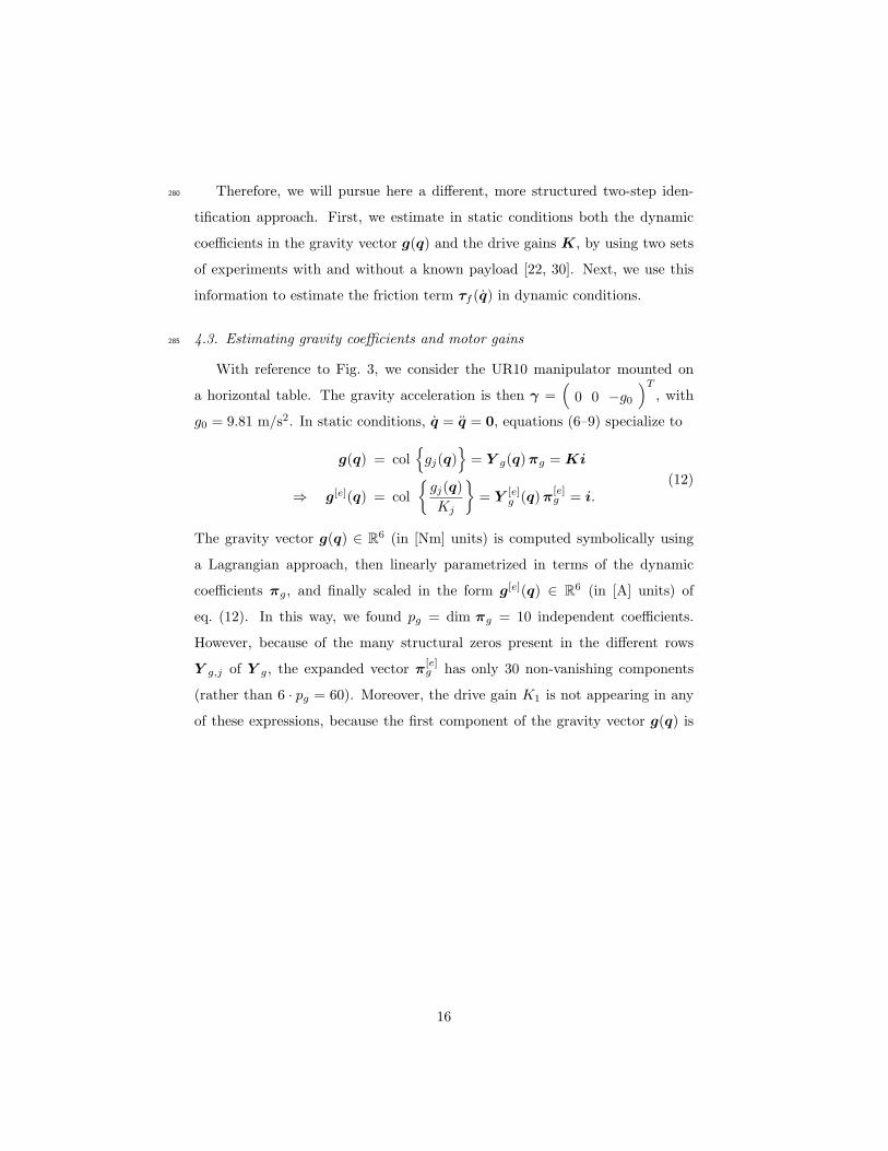
manufacturer data (the peaks of these differences are in the order of 5–6 [A]

on the main joints). Note also that for joint 1 we always get a zero estimate295

for the gravity term, while the current measures are slightly different from zero.

This may be caused by an unmodelled static friction effect at q = 0. A similar

mismatch is present for joint 6 as well.

The same identification procedure has been performed in order to estimate

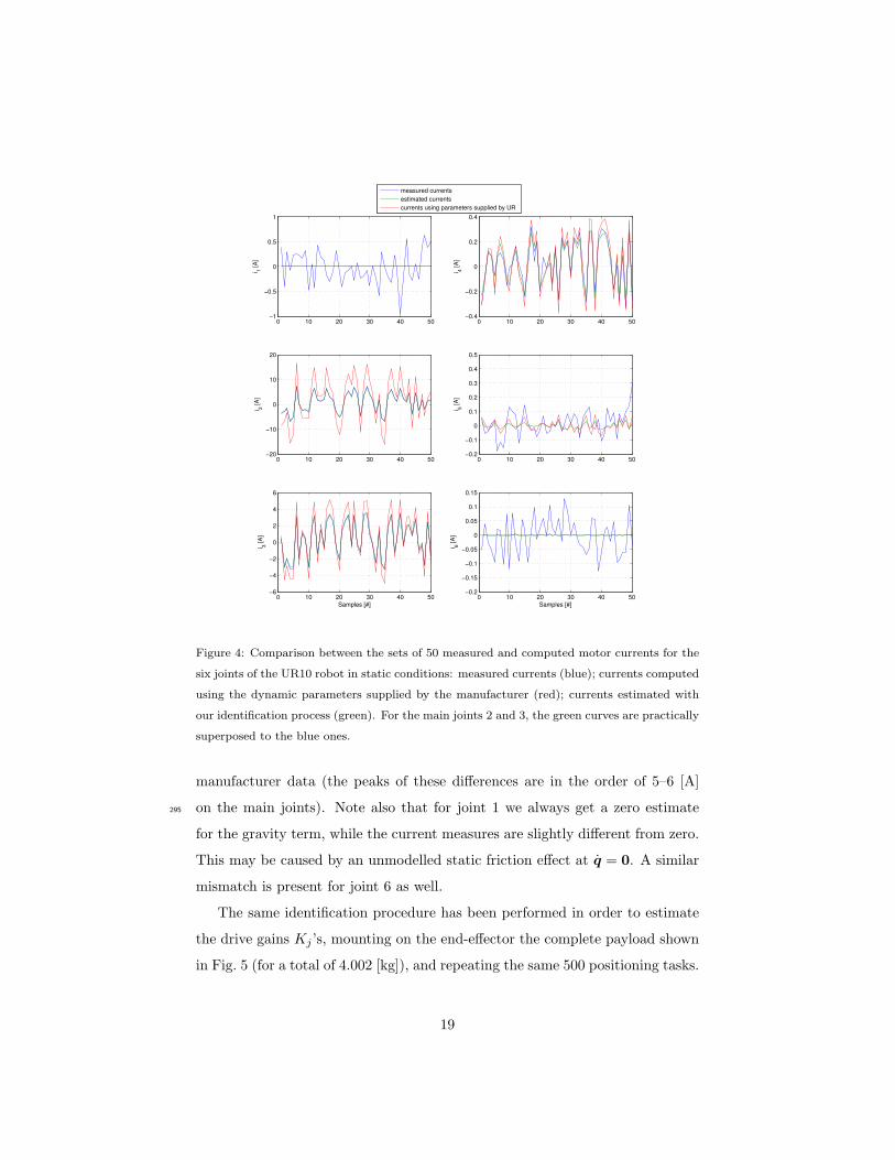
the drive gains Kj ’s, mounting on the end-effector the complete payload shown

in Fig. 5 (for a total of 4.002 [kg]), and repeating the same 500 positioning tasks.

19

2 kg

1 kg

12 cm

15 cm

900 g

4.5 cm

102 g

x6= x

L

z6= z

L y6 = y

L

UR10 5th link

tip

UR10 6th link

Figure 5: The payload parts used for identifying the motor gains (left). A scheme with the

payload reference frame, which is coincident with the frame of the sixth link (right).

In the presence of a payload, the extended vector π[e]g is modified to the loaded

one π[e]g,L, using the following substitutions in the dynamic coefficients

c6vm6 → c6vm6 + cLvmL, v = x, y, z, (15)

where the mass and the position of the center of mass of the sixth (last) link of

the UR10 and of the payload are denoted as mk and ck =(ckx cky ckz

)T,300

respectively for k = 6 and k = L. At the end of the procedure, a new estimation

π[e]g,L is obtained, and the numerical difference ε[e]

g,L = π[e]g,L − π

[e]g is computed.

Since the symbolic difference vector ε[e]g,L = π

[e]g,L − π

[e]g contains the five

scalars Kj , j = 2, . . . , 6, as the only unknowns3, their estimation is set up as

follows. Define

K† =(

1K2

. . .1K6

)T. (16)

By linearity, we can introduce a Jacobian matrix Jεg, evaluated with the known

payload data, and write

JεgK† = ε

[e]g,L, with Jεg

=∂ε

[e]g,L

∂K†. (17)

3Based on the structure of the coefficients ξj in (13) and on their modifications (15), the

symbolic difference vector ε[e]g,L will have only 17 non-vanishing components. Numerical values

for estimation are assigned only to these.

20

0 2 4 6 8 10−5

−4

−3

−2

−1

0

1

2

3

4

5

time [s]

i 1 [

A]

without payload

with payload

0 2 4 6 8 10−2

−1.5

−1

−0.5

0

0.5

1

1.5

2

2.5

time [s]

i 1 d

iffe

ren

ce

[A

]

measured current

filtered current

Figure 6: Motor currents at joint 1 during an exciting trajectory, without (blue) and with

(red) a payload [left]. Difference of the measured currents and its filtered version [right].

The (inverse of the) drive gains are estimated by pseudoinversion as

K†

= J#ε ε

[e]g,L ⇒ K =

( 1

K†2. . .

1

K†6

)T. (18)

The following estimates were obtained for the drive gains of the joints that are

subject to gravity in the UR10 manipulator4:

K2 = 13.26, K3 = 11.13, K4 = 10.62, K5 = 11.03, K6 = 11.47 [Nm/A].

(19)

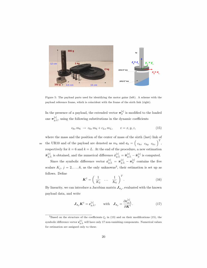
In order to estimate the missing drive gain K1 of joint 1, where no gravity is

felt, a dynamic rather than static procedure was needed, including again pairs

of experiments with and without payload. To maximize the inertial effects of

the payload on joint 1, trajectories were designed that move only the first joint

and keep all the others at rest, with the arm straight and almost parallel to

the ground. Figure 6 shows the measured motor currents during one of these

trajectories, with and without the known payload, and their filtered difference.

The motor gain of joint 1 was finally estimated as:

K1 = 14.87 [Nm/A]. (20)

4 Note that an asymmetric payload has been used additionally for estimating the gain K6

of the last motor, in order to produce a gravitational torque around the last joint axis.

21

4.4. Estimating motor friction

After estimating the gravity vector and the diagonal matrix of drive gains, we

have used the inertial parameters of the six links of the UR10 robot reported by

the manufacturer in [25], suitably modified in order to be expressed consistently

with the DH frames of Fig. 3, to obtain an estimate M(q) of the inertia matrix.

From this, by means of the Christoffel symbols [28], we derive also an estimate

of the Coriolis and centrifugal matrix C(q, q). Since we have an estimate of the

drive gains, we can now determine the contribution of these dynamic terms to

the motor currents associated to a desired trajectory. In fact, the jth equation

in (7) can be rewritten more explicitly as

M j(q)Kj

q +Cj(q, q)Kj

q +gj(q)Kj

= ij , (21)

where M j and Cj are 6-dimensional row vectors, while gj , Kj and ij are scalar

quantities. Combining the assumed inertial data with the previously estimated

gravity vector g[e](q) in (14) and estimated drive gains K in (19) and (20), we

get the following estimation of the motor currents along a twice differentiable

motion q(t):

ij =M j(q)Kj

q +Cj(q, q)Kj

q +gj(q)Kj

, j = 1, . . . , 6. (22)

As a first validation experiment, we imposed the sinusoidal joint trajectories

qj(t) = −(π/2)+(π/4) sin ((π/20)t), for j = 2, 4, and qj(t) = (π/4) sin ((π/20)t),305

for j = 1, 3, 5, 6, and performed a comparison between the motor currents es-

timated by (22) and the measured currents, filtered through a 4th-order zero-

phase digital Butterworth filter with a cutoff frequency of 1 Hz. Figure 7 shows

that the remaining differences are still non-negligible, namely of the order of

0.4–1.4 [A] depending on the joint. We also noticed that the motor currents310

typically change sign together with the relative joint velocities, a fact that is

especially evident for the first and last two joints, while they display in general

a small but sharp discontinuity close to the zero-velocity regime. These behav-

iors can be attributed to friction effects at the motors/transmissions that are

velocity dependent.315

22

0 10 20 30 40 50 60−2

−1

0

1

2

time [s]

i 1 [

A]

0 10 20 30 40 50 60−10

−5

0

5

10

time [s]

i 2 [

A]

0 10 20 30 40 50 60−5

0

5

time [s]

i 3 [A

]

0 10 20 30 40 50 60−1

−0.5

0

0.5

1

time [s]

i 4 [A

]

0 10 20 30 40 50 60−0.4

−0.2

0

0.2

0.4

time [s]

i 5 [

A]

0 10 20 30 40 50 60−0.4

−0.2

0

0.2

0.4

time [s]

i 6 [

A]

Estimated currents

Measured currents

Figure 7: Comparison between measured (green, dashed) and estimated (blue, continuous)

motor currents, neglecting friction.

Therefore, we proceeded with an estimation of the motor currents (in [A])

associated to the friction torque τf (q) (in [Nm]) in eq. (1), assuming this last

missing term as a function of the joint velocity. In order to derive a functional

model for the motor friction, we executed several rest-to-rest cubic trajectories

having different maximum speed, moving one joint at the time and keeping the

others at rest. For every joint j ∈ {1, . . . , 6}, we collected on the average 10k

samples of the motor current. Eventually, we found that the best model that

fits the data was given by a sigmoidal function added to an affine function as

τf,j(qj)Kj

= (aj qj + bj) +Sj

1 + e−αj(qj+νj). (23)

This function is characterized by five parameters aj , bj , Sj , αj , and νj . These

were estimated solving a nonlinear least squares problem by means of a Nelder-

Mead routine, using as fitting data the differences between the measured motor

23

−1.5 −1 −0.5 0 0.5 1 1.5−10

−5

0

5

10

J1 velocity [rad/s]

i me

as −

i est

[A

]

−1.5 −1 −0.5 0 0.5 1 1.5−10

−5

0

5

10

J2 velocity [rad/s]

i me

as −

i est

[A

]

−1.5 −1 −0.5 0 0.5 1 1.5−5

0

5

J3 velocity [rad/s]

i me

as −

i est

[A

]

−1.5 −1 −0.5 0 0.5 1 1.5−1

−0.5

0

0.5

1

J4 velocity [rad/s]

i me

as −

i est

[A

]

−1.5 −1 −0.5 0 0.5 1 1.5−1

−0.5

0

0.5

1

J5 velocity [rad/s]

i me

as −

i est

[A

]

−1.5 −1 −0.5 0 0.5 1 1.5−1

−0.5

0

0.5

1

J6 velocity [rad/s]

i me

as −

i est

[A

]

friction estimationcurrent difference

Figure 8: The estimated friction functions (23) for the six UR10 robot joints. The data to fit

(green dots) are the differences between measured and estimated currents.

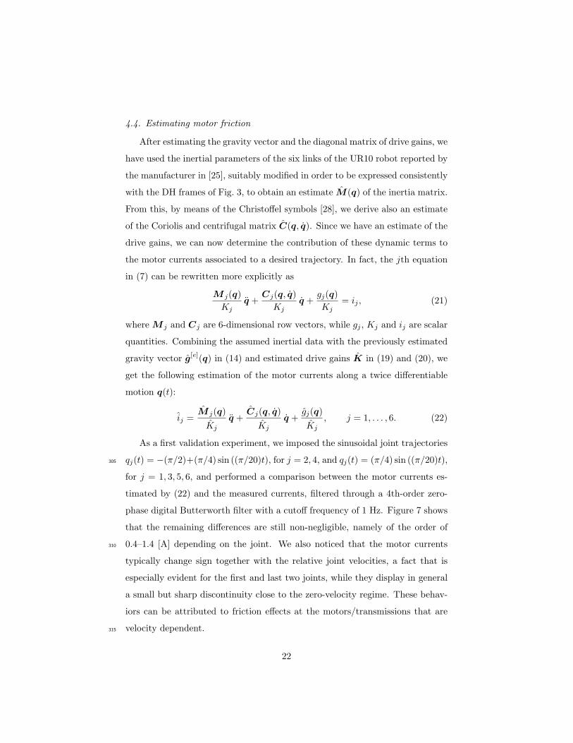
currents and the estimated currents ij given by (22). For the six joints of the

UR10 robot, we have identified a total of 30 structural parameters for friction.320

The plots of the obtained friction functions are shown in Fig. 8.

Adding the estimated current components due to friction, we finally obtained

the following estimation of the total motor current for each joint j:

ij =M j(q)Kj

q +Cj(q, q)Kj

q +gj(q)Kj

+τf,j(q)Kj

, j = 1, . . . , 6. (24)

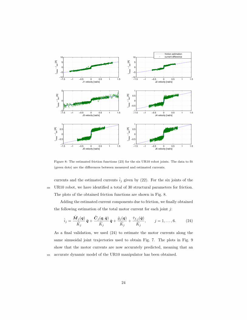
As a final validation, we used (24) to estimate the motor currents along the

same sinusoidal joint trajectories used to obtain Fig. 7. The plots in Fig. 9

show that the motor currents are now accurately predicted, meaning that an

accurate dynamic model of the UR10 manipulator has been obtained.325

24

0 10 20 30 40 50 60−1.5

−1

−0.5

0

0.5

1

1.5

time [s]

i 1 [A]

0 10 20 30 40 50 60−20

−10

0

10

20

time [s]

i 2 [A]

0 10 20 30 40 50 60−6

−4

−2

0

2

4

6

time [s]

i 3 [A]

0 10 20 30 40 50 60−1

−0.5

0

0.5

1

time [s]i 4 [A

]

0 10 20 30 40 50 60−0.4

−0.2

0

0.2

0.4

0.6

time [s]

i 5 [A]

0 10 20 30 40 50 60−0.4

−0.2

0

0.2

0.4

time [s]

i 6 [A]

Estimated currentsMeasured currentsCurrents using parameters supplied by UR

Figure 9: Measured (green, dashed) and estimated (blue, continuous) motor currents, includ-

ing friction. For comparison, we report also the motor currents (red, continuous) computed

using the dynamic parameters supplied by the manufacturer [25]; these currents are clearly

different from the measured and our estimated ones.

4.5. Collision detection test

The quality of the outcome of the identification process described in Sec. 4.3–

4.4 has been further tested by verifying if and how one is able to detect possible

collisions between a human operator and the UR10 manipulator while the robot

is in motion, when using our estimated dynamic model.330

Figure 10 shows the evolution of the six components of the residual r in

eq. (3), when two almost instantaneous and mild contact forces are exerted

along opposite Cartesian directions on link 3, respectively at the time instants

t = 45 s and t = 65 s. The nominal sinusoidal motion of the joints was the

same used to obtain the currents in Fig. 7. The two peaks at joints 2 and 3 are335

25

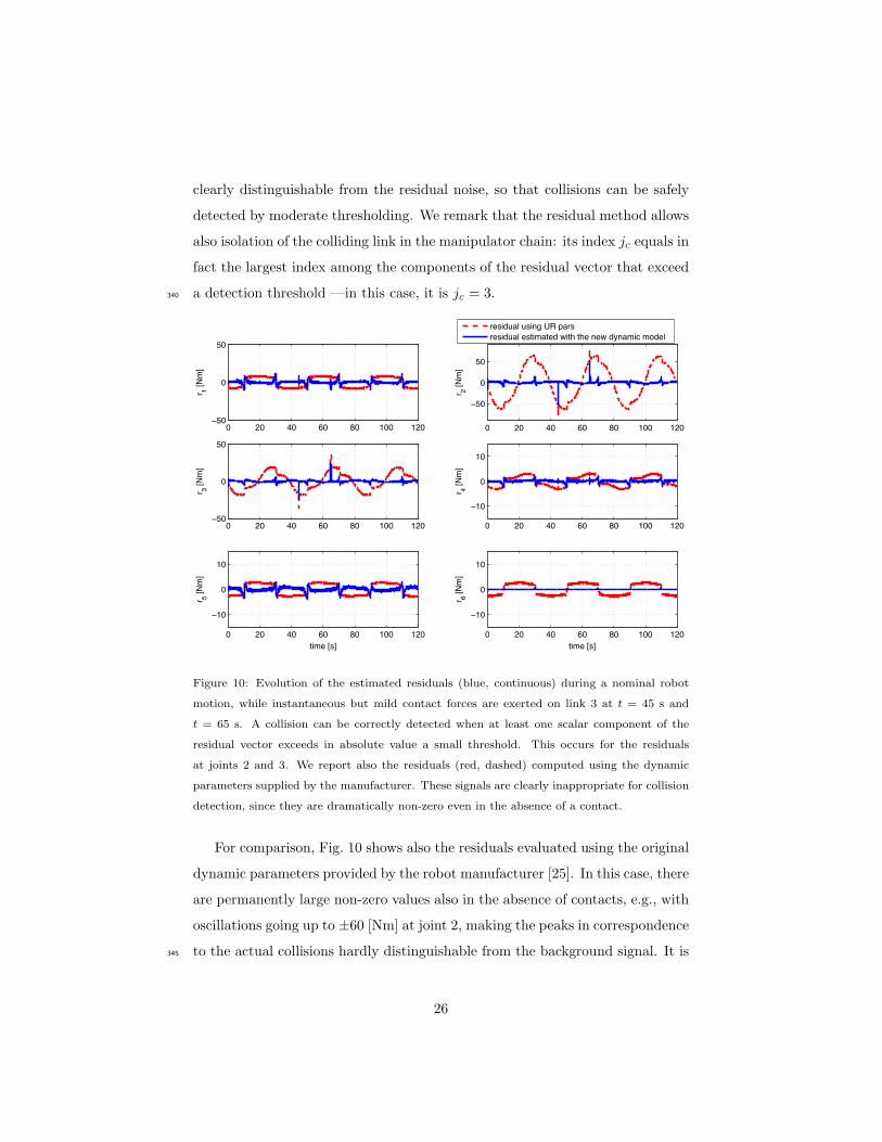
clearly distinguishable from the residual noise, so that collisions can be safely

detected by moderate thresholding. We remark that the residual method allows

also isolation of the colliding link in the manipulator chain: its index jc equals in

fact the largest index among the components of the residual vector that exceed

a detection threshold —in this case, it is jc = 3.340

0 20 40 60 80 100 12050

0

50

r 1 [Nm

]

0 20 40 60 80 100 120

50

0

50

r 2 [Nm

]

0 20 40 60 80 100 12050

0

50

r 3 [Nm

]

0 20 40 60 80 100 120

10

0

10r 4 [N

m]

0 20 40 60 80 100 120

10

0

10

time [s]

r 5 [Nm

]

0 20 40 60 80 100 120

10

0

10

time [s]

r 6 [Nm

]

residual using UR parsresidual estimated with the new dynamic model

Figure 10: Evolution of the estimated residuals (blue, continuous) during a nominal robot

motion, while instantaneous but mild contact forces are exerted on link 3 at t = 45 s and

t = 65 s. A collision can be correctly detected when at least one scalar component of the

residual vector exceeds in absolute value a small threshold. This occurs for the residuals

at joints 2 and 3. We report also the residuals (red, dashed) computed using the dynamic

parameters supplied by the manufacturer. These signals are clearly inappropriate for collision

detection, since they are dramatically non-zero even in the absence of a contact.

For comparison, Fig. 10 shows also the residuals evaluated using the original

dynamic parameters provided by the robot manufacturer [25]. In this case, there

are permanently large non-zero values also in the absence of contacts, e.g., with

oscillations going up to ±60 [Nm] at joint 2, making the peaks in correspondence

to the actual collisions hardly distinguishable from the background signal. It is345

26

quite evident that these untuned residuals are completely useless, since collision

events are almost completely masked and intentional contact forces applied by

the user would not be correctly recognized.

We note finally that the estimated residuals still exhibit small peaks when-

ever the joint velocity changes sign. This could be due to yet unmodeled dissi-350

pative effects, such as a larger static and Stribeck friction, with respect to those

captured by the model equation (23).

5. HRC experimental results

We present here some experimental results of the proposed control law (5)

applied to the Universal Robot UR10 manipulator. The hardware platform355

was a 64-bit Intel Core i7-6700K CPU, equipped with 16GB DDR4 RAM. The

complete process of residual computation and motion control runs on the robot

at 8 ms cycle time. In order to measure the external force F e applied by the

human, the robot is equipped with an ATI Mini45 6D Force/Torque sensor,

mounted on its end-effector. With reference to the residual computation (3),360

the gain matrix G has been chosen as G = 3.6 · I6, where Ik denotes the k× k

identity matrix. The other parameters in (5) were set to Kp = 2.3 · I3 and

Kr = 0.16 · I6. Finally, the desired constant position pd for the mimicked

polishing task operation has been chosen as pd = (−0.07 0.89 0.31)T [m]

with respect to the base frame in Fig. 3.365

During the proposed interaction experiment, the human pushes the robot at

the end-effector level and/or along its structure to emulate a polishing process

and the need to reorient the polished part. Figures 11–13 show snapshots of

the various phases of the experiment, while Figure 14 reports the time behavior

of different variables during the task: the robot end-effector position p ∈ R3,370

the joint position variables q ∈ R6, only the end-effector contact force fe ∈ R3

measured by the F/T sensor, and the residual vector r ∈ R6 computed as (3).

Due to uncertainties left in the dynamic model or unmodeled effects, and in order

to keep limited the effects of noise in the motor current sensor, the residual vector

27

has been considered to be zero if ‖r‖ ≤ rth, a threshold set to rth = 10 [Nm].375

The reported experiment can be seen in the accompanying video clip (also on

YouTube at https://youtu.be/bjZbmlAclYk).

By comparing the plots of the variables of interest in Fig. 14 with the snap-

shots/video, one can distinguish different human-robot collaboration phases.

• In the interval 4 s ≤ t ≤ 8 s, only the polishing force is exerted, which is380

completely represented by the force sensor measure, since no contact along

the robot structure occurs (Fig. 11). As expected, position and orientation

of the end-effector do not change and there is no joint motion. In fact, the

control law counterbalances all manual polishing forces/torques applied by

the operator. Note that, the residual vector remains equal to zero during385

this phase.

• When 10 s ≤ t ≤ 15 s, the operator pushes only on the robot structure.

The contact is detected by the residual and the robot joints move according

to eq. (5), relaxing the end-effector orientation. Thanks to the null-space

projection, the end-effector position remains constant even if the joint390

configuration changes. In this way, the robot arm can be reconfigured by

the operator so as to reorient the held workpiece in the most comfortable

way. Figure 12 shows this situation.

• When 16 s ≤ t ≤ 22 s, both a polishing force and an extra contact

force/moment (on the robot structure) are exerted at the same time. Here,395

the joints move only due to the resulting extra joint torque detected by

the residual. Still, the control law counterbalances all manual polishing

forces/torques applied by the operator, as shown in Fig. 13.

Similar considerations can be done for the remaining parts of the experiment.

6. Conclusions400

We have addressed a human-robot collaboration problem that arises in the

robot-aided industrial task of abrasive surface polishing for metallic workpieces

with complex geometry. We presented a control scheme that allows a human

28

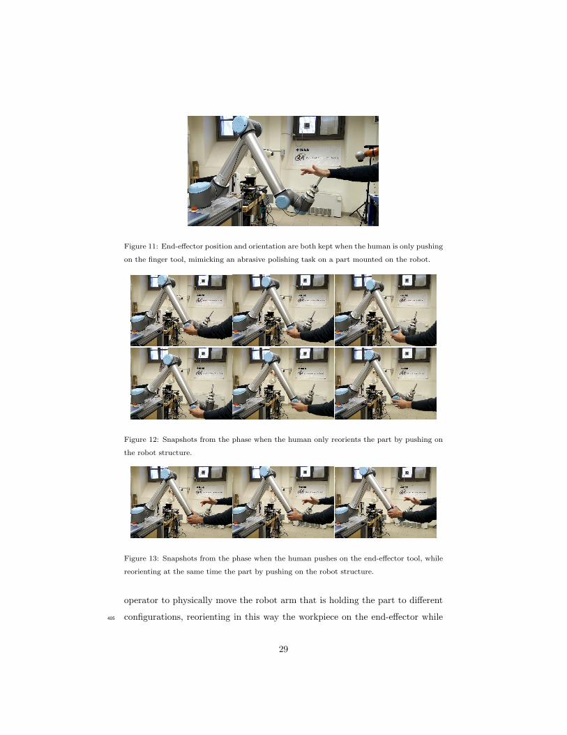
Figure 11: End-effector position and orientation are both kept when the human is only pushing

on the finger tool, mimicking an abrasive polishing task on a part mounted on the robot.

Figure 12: Snapshots from the phase when the human only reorients the part by pushing on

the robot structure.

Figure 13: Snapshots from the phase when the human pushes on the end-effector tool, while

reorienting at the same time the part by pushing on the robot structure.

operator to physically move the robot arm that is holding the part to different

configurations, reorienting in this way the workpiece on the end-effector while405

29

0 5 10 15 20 25 30 35 40 45−0.2

0

0.2

0.4

0.6

0.8

1

1.2

EE

Position[m

]

px py pz

0 5 10 15 20 25 30 35 40 45−3

−2

−1

0

1

2

3

JointPosition

[rad]

q1 q2 q3 q4 q5 q6

0 5 10 15 20 25 30 35 40 45−100

−80

−60

−40

−20

0

20

40

EE

Force

[N]

Fx Fy Fz

0 5 10 15 20 25 30 35 40 45−15

−10

−5

0

5

10

15

20

Residual

[Nm]

Time [s]

r1 r2 r3 r4 r5 r6

Figure 14: Human-robot collaborative experiment. From the top: end-effector Cartesian

position, joint position variables, contact force at the end-effector measured by the F/T sensor,

and components of the residual vector.

30

keeping instead fixed its position so as to better accomplish manual polishing.

This robot behavior can be realized without extra interfaces (e.g., a touch screen

or teach-pendant), by simply pushing the arm structure in a very natural way

and implementing an admittance control law with a null-space algorithm to

exploit kinematic redundancy of the task. The robot reconfiguration is obtained410

in the same way both if the operator has paused the activity or if is still exerting

at the same time a polishing force on the workpiece. This decoupling is made

possible by the simultaneous use of a standard force/torque sensor mounted on

the robot wrist and of our model-based dynamic method of residuals, which

estimates the joint torques associated to contact forces/moments applied at415

any location of the manipulator arm. We proved our algorithm with good

results on a UR10 lightweight robot, mounting a small-size 6D F/T sensor and

using otherwise the original low-level motion controller that accepts user-defined

kinematic commands. A major subtask was to estimate an accurate dynamic

model of the manipulator, including the significant friction effects and the motor420

current-to-torque gains, in order to compute a reliable residual signal.

Our current work within the SYMPLEXITY project is devoted to integra-

tion activities of this human-robot collaborative scheme into the actual manual

abrasive polishing station of the industrial cell for robotized laser polishing, in-

corporating it in the overall process control flow and the available HMI and425

protocols, and using the two Kinects that monitors the safe human-robot coex-

istence also for improving the physical collaboration phase.

References

[1] Y. Lu, Industry 4.0: A survey on technologies, applications and open re-

search issues, J. of Industrial Information Integration 6 (2017) 1–10.430

[2] A. De Santis, B. Siciliano, A. De Luca, A. Bicchi, An atlas of physical

human-robot interaction, Mechanism and Machine Theory 43 (3) (2008)

253–270.

[3] A. De Luca, F. Flacco, Integrated control for pHRI: Collision avoidance,

31

detection, reaction and collaboration, in: Proc. IEEE Int. Conf. on Biomed-435

ical Robotics and Biomechatronics, 2012, pp. 288–295.

[4] A. De Luca, R. Mattone, Sensorless robot collision detection and hybrid

force/motion control, in: Proc. IEEE Int. Conf. on Robotics and Automa-

tion, 2005, pp. 1011–1016.

[5] A. De Luca, A. Albu-Schaffer, S. Haddadin, G. Hirzinger, Collision detec-440

tion and safe reaction with the DLR-III lightweight robot arm, in: Proc.

IEEE/RSJ Int. Conf. on Intelligent Robots and Systems, 2006, pp. 1623–

1630.

[6] S. Haddadin, A. De Luca, A. Albu-Schaffer, Robot collisions: A survey

on detection, isolation, and identification, IEEE Trans. on Robotics 33 (6)445

(2017) 1292–1312.

[7] F. Flacco, T. Kroger, A. De Luca, O. Khatib, A depth space approach for

evaluating distance to objects – with application to human-robot collision

avoidance, J. of Intelligent & Robotic Systems 80, Suppl. 1 (2015) 7–22.

[8] F. Flacco, A. De Luca, Real-time computation of distance to dynamic ob-450

stacles with multiple depth sensors, IEEE Robotics and Automation Lett.

2 (1) (2017) 56–63.

[9] ISO 10218-1-2011, Robots and robotic devices – Safety requirements for

industrial robots. Part 1: Robots; Part 2: Robot systems and integration

(since July 1, 2011).455

URL http://www.iso.org

[10] ISO TS 15066:2016, Robots and robotic devices – Collaborative robots

(since February 15, 2016).

URL http://www.iso.org

[11] L. Lucignano, F. Cutugno, S. Rossi, A. Finzi, A dialogue system for mul-460

timodal human-robot interaction, in: Proc. 15th ACM Int. Conf. on Mul-

timodal Interaction, 2013, pp. 197–204.

32

[12] S. Iengo, S. Rossi, M. Staffa, A. Finzi, Continuous gesture recognition for

flexible human-robot interaction, in: Proc. IEEE Int. Conf. on Robotics

and Automation, 2014, pp. 4863–4868.465

[13] A. Stolt, A. Robertsson, R. Johansson, Robotic force estimation using

dithering to decrease the low velocity friction uncertainties, in: Proc. IEEE

Int. Conf. on Robotics and Automation, 2015, pp. 3896–3902.

[14] A. Colome, D. Pardo, G. Alenya, C. Torras, External force estimation dur-

ing compliant robot manipulation, in: Proc. IEEE Int. Conf. on Robotics470

and Automation, 2013, pp. 3535–3540.

[15] E. Berger, S. Grehl, D. Vogt, B. Jung, H. Amor, Experience-based torque

estimation for an industrial robot, in: Proc. IEEE Int. Conf. on Robotics

and Automation, 2016, pp. 144–149.

[16] A. Vick, D. Surdilovic, J. Kruger, Safe physical human-robot interaction475

with industrial dual-arm robots, in: Proc. 9th IEEE Int. Work. on Robot

Motion and Control, 2013, pp. 264–269.

[17] A. Cirillo, F. Ficuciello, C. Natale, S. Pirozzi, A conformable force/tactile

skin for physical human-robot interaction, IEEE Robotics and Automation

Lett. 1 (1) (2016) 41–48.480

[18] E. Magrini, F. Flacco, A. De Luca, Estimation of contact forces using a

virtual force sensor, in: Proc. IEEE/RSJ Int. Conf. on Intelligent Robots

and Systems, 2014, pp. 2126–2133.

[19] E. Magrini, F. Flacco, A. De Luca, Control of generalized contact motion

and force in physical human-robot interaction, in: Proc. IEEE Int. Conf.485

on Robotics and Automation, 2015, pp. 2298–2304.

[20] E. Magrini, A. De Luca, Hybrid force/velocity control for physical human-

robot collaboration tasks, in: Proc. IEEE/RSJ Int. Conf. on Intelligent

Robots and Systems, 2016, pp. 857–863.

33

[21] C. Gaz, F. Flacco, A. De Luca, Identifying the dynamic model used by the490

KUKA LWR: A reverse engineering approach, in: Proc. IEEE Int. Conf.

on Robotics and Automation, 2014, pp. 1386–1392.

[22] C. Gaz, A. De Luca, Payload estimation based on identified coefficients

of robot dynamics –with an application to collision detection, in: Proc.

IEEE/RSJ Int. Conf. on Intelligent Robots and Systems, 2017, pp. 3033–495

3040.

[23] SYMPLEXITY, Symbiotic Human-Robot Solutions for Complex Surface

Finishing Operations.

URL www.symplexity.eu

[24] Coppelia Robotics, v-rep virtual robot experimentation platform (2015).500

URL http://www.coppeliarobotics.com

[25] Universal Robots, Universal Robots Offline Simulator.

URL https://www.universal-robots.com/download/?option=28545#

section16632

[26] Universal Robots, The URScript Programming Language, version 3.1505

(2015).

[27] J. Swevers, W. Verdonck, J. De Schutter, Dynamic model identification for

industrial robots, IEEE Control Systems Mag. 27 (5) (2007) 58–71.

[28] B. Siciliano, L. Sciavicco, L. Villani, G. Oriolo, Robotics: Modeling, Plan-

ning and Control, 3rd Edition, Springer, London, 2008.510

[29] W. Khalil, E. Dombre, Modeling, Identification and Control of Robots,

Hermes Penton London, 2002.

[30] M. Gautier, S. Briot, Global identification of drive gains parameters of

robots using a known payload, in: Proc. IEEE Int. Conf. on Robotics and

Automation, 2012, pp. 2812–2817.515

34