1

A Model-Based Indicator of Musculoskeletal Disorders

via Hidden Markov Models

as an EMG Pattern Recognition Method

(First Draft)

A FINAL PAPER SUBMITTED IN PARTIAL FULFILLMENT OF THE REQUIREMENTS FOR THE

INDEPENDENT RESEARCH PROJECT

STA4000Y

PROFESSOR JEFFREY ROSENTHAL DEPARTMENT OF STATISTICS

Anjali Mazumder 950116380

December 2003

2

Acknowledgements

Dr. Donald Cole, Dr. Sheilah Hogg-Johnson, and Dwayne VanEerd for the opportunity to work on this interesting project and allowing me to explore areas of interest.

Professor J. Rosenthal for the opportunity to explore this field and most importantly for being patient for taking my time to learn, understand and make

use of it.

3

Table of Contents List of Figures: .................................................................................................................. 4 List of Abbreviations........................................................................................................ 5 Section 1: Introduction .............................................................................................. 6

1.1 Use of HMMs........................................................................................................... 6 1.2 Motivation ......................................................................................................... 7 1.3 Overview ............................................................................................................ 7 1.4 Data and Software ............................................................................................ 8

Section 2: Hidden Markov Models for a Single Process ....................................... 9 2.1 Elements of a HMM ......................................................................................... 9 2.2 Model Generation and Definition of an HMM .......................................... 10 2.3 Assumptions in the Theory of HMMs ......................................................... 11 2.4 Some Theoretical Aspects and Consequences of ....................................... 13 Assumptions in HMM Theory .................................................................................. 13 2.5 Summary Remarks......................................................................................... 14

Section 3: Types of Hidden Markov Models ......................................................... 15 3.1 Left-Right Model ............................................................................................ 15 3.2 Continuous and Semi-continuous HMMs .................................................. 17 3.3 Autoregressive (AR) HMMs ......................................................................... 18 3.4 Representation of HMMs.............................................................................. 20 3.5 Other Remarks................................................................................................ 22

Section 4: Computational Methods for HMMs .................................................... 23 4.1 The Three Fundamental Problems for HMMs........................................... 23 4.2 The Evaluation Problem................................................................................ 24 4.3 The Decoding Problem and Pattern Recognition ...................................... 26 4.4 The Learning Problem ................................................................................... 27 4.5 Other Remarks................................................................................................ 30

Section 5: HMMs for EMG Pattern Recognition ................................................. 31 5.1 Rationale/Background .................................................................................. 31 5.2 EMG Signal Processing ................................................................................. 32 5.3 Methods and Analysis.................................................................................... 33 5.4 Preliminary Results and Discussion............................................................ 35 5.5 Proposed Framework for an EMG Pattern Recognition Method............ 37

Section 6: Concluding Remarks.............................................................................. 39 References ....................................................................................................................... 40

4

List of Figures Figure 1: A typical graphical representation of an HMM 13 Figure 2: An HMM with parameters explicitly represented 21 Figure 3: HMMs with mixture of Gaussian outputs 21 Figure 4: HMMs with semi-tied mixtures 21 Figure 5: Autoregressive HMMs 22 Figure 6: Graphical Depiction of EMG chunking method 35 Figure 7: Static level of EMG for keying versus not keying 36 Figure 8: EMG levels for optimal versus non-optimal mouse 37

5

List of Abbreviations AR autoregressive models CPD conditional probability distribution DBNs dynamic Bayesian networks ECRB extensor carpi radialis brevis EMG electromyographical signals HMMs hidden Markov models MDS multidimensional scaling ML maximum likelihood MMI maximum mutual information MVC maximum voluntary contraction PMF probability mass function PDF probability density function WMSDs work-related musculoskeletal disorders iid independent identically distributed rv random variables wrt with respect to

6

Section 1: Introduction Sequential data is a common attribute or form of “real-world” processes found in all areas of science and engineering. Hidden Markov models (HMMs) provide a flexible means of modeling the behavior of such natural processes. Its mathematically tractable form allows for these processes to be discrete or continuous in nature and can be characterized as signals. Such signals possess different traits – pure or distorted, stationary or non-stationary, for example. These properties of the signal can be used to model the specific form of a signal (random) process. This paper focuses on the class of models referred to as hidden Markov models which tries to characterize the statistical properties of a stochastic process and demonstrate their applicability to “real-world” processes.

1.1 Use of HMMs Hidden Markov models hold a fundamental interest in a wide range of applications. Though there are several reasons why such models are of interest, in general, these models are used for two purposes. Prediction systems are commonly employed HMMs in the field of speech recognition, medical prognosis and financial arenas. HMMs are widely used as a pattern recognition method for gene recognition, word recognition in speech processing, visual and gesture recognition, and in various other capacities. HMMs also provide a means of describing the dynamical structure of real-world process. In this capacity, HMMs capture over-dispersion in the observed data which is attributed to the assumption that the observations from one of several marginal distribution, each associated with a hidden state. HMMs provide a natural modeling of the process, especially when a physical meaning can be attributed to the states. Another important use of HMMs is their potential in describing the structure such that the source would not have to be available. Thus, given a good model, the source could be simulated and still maintain the ability to learn as much about the source and the process it outputs via simulations. This attribute is particularly important and of interest to researchers using signal processes (especially) since the cost of a signal process from an actual source is quite high.

7

1.2 Motivation

Electromyographical (EMG) signals are another source of data which may be appropriately modeled by HMMs. EMG signals or simply EMG are often used as an interface device, since they are electrical simulations which indicate the activity level of motor units associated with muscle contractions. Different motions resulting from different muscle activities generate different EMG patterns. Many researchers have used EMG signals in a variety of applications in the medical field including prosthetic control and musculoskeletal disorders (MSDs). Exposures associated with work-related musculoskeletal disorders (WMSDs) have not been clearly defined as there are many factors which are considered “risks”. All jobs involve certain tasks which take a certain amount of time. Some jobs may have tasks which are considered to be more detrimental than others with respect to (w.r.t) developing a WMSD, such as repeated tasks. Some tasks may also be impeded by other physical attributes of the office environment which may be quantified via dimension and posture measures. Many researchers have tried to use EMG signals to determine the differences in muscle load for different tasks. EMG signals provide a valuable understanding in the effects of different risks on muscle activity. However, studies tend to use more conventional modeling approaches to determine differences in performance. In most instances, studies with EMG data are small in number as they are an extremely costly process to output. Hence, hidden Markov models provide a valuable resource in modeling EMG signals and in uncovering the dynamical structure of correlated multivariate time series model. Some studies have used autoregressive (AR) models to represent the EMG signal when measured from a single electrode site while others have used a multi-dimensional AR models to discriminate between various forearm motions (Bu et. al., 2003). Moore et. al. (2003) used simple generalized linear models. The study of HMMs is obviously not new and there is much theory available in the area of obtaining maximum likelihood estimates and various other algorithmic approaches for HMMs. However, there is much gap in both the use of HMMs in modeling EMG and in handling multiple processes (time series) with time-variant observations. This research paper attempts to demonstrate the use of HMMs for EMG signals as a pattern recognition method in understanding the dynamical structure induced by WMSDs. This paper does not attempt to solve the problem but introduces the concept of HMMs to show their applicability to EMG data.

1.3 Overview This paper is partitioned into four core sections. Section 2 introduces hidden Markov models for a single observed process. It also concentrates on presenting some of the theoretical aspects and underpinnings of HMM theory. Section 3 is an extension of the standard HMM introduced in section 2 as it considers continuous and autoregressive

8

models. HMMs and their variants are also formulated as left-right models (as opposed to ergodic or other forms) which is essential in representing HMMs as probabilistic graphical models. Section 4 forms the crux of HMM methodology as it exposes the fundamental problems of interest for HMMs and provides mathematical formulations for the solutions to these problems. Section 5 introduces the concept of using EMG signals as another source of data which can be modeled by HMMs within the context of understanding the dynamical structure imposed by WMSDs. The concluding section proposes further work in the application of HMMs to EMG as a pattern recognition method.

1.4 Data and Software The data used in the application setting of this paper were provided by the Institute for Work & Health which focuses on research in the prevention of injury in the workplace. The data in this study was obtained from a large newspaper office in Southern Ontario. The EMG data used in this study was collected in the summer of 2000. Permission for use of the data was obtained from the principal investigator Dr. Donald Cole (Professor in Public Health Sciences, University of Toronto) and from the author’s supervisor and senior statistician at the Institute for Work & Health, Dr. Sheilah Hogg-Johnson (Professor of Biostatistics, University of Toronto). The software used to clean and prepare the data was SAS. S-plus was used for much of the analysis steps. Brian Ripley’s function for cluster analysis, pattern recognition and neural networks were implemented. For experimental purposes, MATLAB and toolboxes developed by Kevin Murphy were used in implementing HMM algorithms.

9

Section 2: Hidden Markov Models for a Single Process This section provides a formal definition of a HMM for a single process. Some of the underlying assumptions relevant to the theoretical presentation are also given. This provides the background and lays the foundation for the structural framework of the model. The purpose of this section is to introduce the basic concepts and elements of HMMs and shed insight into possible applications and extensions of such models.

2.1 Elements of a HMM In brief, an HMM is a double stochastic process, denoted λ. That is, HMMs describe the relationship between an observed process and an unobserved (hidden) process. Define tY to be the observed response at time t and tZ be the hidden state at time t. The characterization of an HMM is based on five elements, forming a 5-tuple.

1. N denotes the number of states (which are hidden) in the model. Of interest are the possible interconnections of individual states denoted },...,{ 1 NSSS = such that any state can be reached from any other state. Let tq denote the state at time t.

2. M denotes the number of distinct observation symbols per state or more explicitly

correspond to the observed response process which is being modeled. Let },...,{ 1 mvvV = denote the set of observation symbols.

3. A state transition probability distribution (set of state transition probabilities), also

called transition matrix }{ ijaA = , representing the probability of going from state

iS to jS .

,,1 ]|[ 1 NjiSqSqPa itjtij ≤≤=== +

where tq denotes the current state. The transition probabilities should also satisfy the normal stochastic constraints,

Njiaij ≤≤> ,1 ,0

10

and

.1 ,11

NiaN

jij ≤≤=∑

=

4. An observation symbol probability distribution, also called emission matrix

)}({ kbB j= , indicating the probability of emission of symbol kv when system state is jS .

MkNSqvoPkb jtktj ≤≤≤≤=== 1 ,j1 },|{)(

where kv denotes the kth observation symbol, and to the current parameter vector. The following stochastic constraints must be satisfied

MkNjkb j ≤≤≤≤≥ 1 ,1 ,0)(

and

.1 ,1)(1

NjkbM

kj ≤≤=∑

=

5. An initial state probability distribution }{ iππ = , representing probabilities of

initial states.

.1 ,0 ,1 ][1

1 ∑=

=≥≤≤==N

iiiii NiSqP πππ

Thus, using conventional notation, there are five key elements of an HMM. However, assuming a fixed N and M, we can define an HMM as a triplet composed of the distributional parameters ),,( πλ BA= .

2.2 Model Generation and Definition of an HMM Before describing the Hidden Markov model, it is necessary to describe the foundation, the Markov process. For brevity purposes, a theoretical discussion on Markov chains is deferred from this paper. However, in simplicity, a sequential pattern usually has a sufficient structure to influence the probability of the next event. A stochastic process is called a jth-order Markov process if the conditional probability density of the current event, given all past and present events, depends only on the j most recent events. More formally, a Hidden Markov model is described as a double stochastic process. It consists of a first stochastic layer which is an underlying first-order Markov process. It

11

models the state transition where each state is a possible observation of the Markov process, and a transition probability from state iS to state jS is )|( 1 itjt SqSqP ==+ , the probability of going to state jS at time t+1 given that the state at time t is iS . The second stochastic layer of the HMM is the set of emission probabilities for each state. For instance, the emission probabilities of state iS specifies the likelihood of seeing certain observations, given the HMM is actually in state iS . This second layer of probabilities creates the image of a veil so that, given a sequence of observations, the actual sequence of states is ambiguous; it is “hidden” from the observer. Recalling the notation previously defined, the five elements of an HMM can be used both as a generator of observations as well as a model for how a given observation sequence can be generated from an appropriate HMM given appropriate values for the 5-tuple. A procedure for such a generation of an observation sequence was given in Rabiner (1989) and is given as follows:

1. Choose an initial state iSq =1 according to the initial state distribution π . 2. Set t = 1.

3. Choose kt vO = according to the symbol probability distribution in state iS , i.e.

)(kbi . 4. Transition to a new state jt Sq =+1 according to the state transition probability

distribution for state iS , i.e. ija .

5. Set 1+= tt ; return to step (3) if Tt < ; otherwise terminate the procedure.

In summary, the hidden Markov model is a finite set of states, each of which is associated with a (generally multidimensional) probability distribution. Transitions among the states are governed by a set of probabilities, commonly referred to as transition probabilities. In a particular state an outcome or observation can be generated, according to the associated probability distribution. It is only the response or output process which is observed while the states are “hidden” or unobserved.

2.3 Assumptions in the Theory of HMMs The mathematically tractable form of hidden Markov models is due to the theoretical underpinnings. Below three of the most common assumptions employed in HMMs are briefly discussed. HMMs are not confined to just these three assumptions and others have relaxed some of these assumptions as well depending on the type of HMM.

12

Perhaps the most palpable assumption is the Markovian assumption. As given in the definition of HMMs, transition probabilities are defined as,

].|[ 1 itjtij SqSqPa === + It is assumed that the next state is dependent only upon the current state. This is called the Markov assumption and the resulting model becomes actually a first order HMM. However, generally the next state may depend on the past k states and it is possible to obtain such a model, referred to as a kth order HMM by defining the transition probabilities as follows.

.,,...,,1 },,...,,|{ 21111,... 2121NjiiiSqSqSqSqPa kiktititjtjiii kk

≤≤===== +−−+

Even though the first-order HMMs are the most common, some attempts have been made to use the higher order HMMs, despite their obvious higher complexity. Another standard assumption in the theory of HMMS is that of the stationarity. }{ tq is a Markov chain with transition probabilities ija and initial probabilities iπ ; and }{ tq is assumed to be stationary. It is assumed that state transition probabilities are independent of the actual time at which the transitions take place. Mathematically, it can be stated as

],|[]|[2211 11 itjtitjt SqSqPSqSqP ===== ++

for any 1t and 2t . The output independence assumption, prominent in HMMs, is the assumption that the current output (observation) is statistically independent of the previous outputs (observations). This assumption can be mathematically formulated by considering a sequence of observations,

ToooO ,..., 21= .

Then according to the parameter triplet of the HMM,

∏=

=T

tttT qoPqqqOP

121 ),|{},,...,,|{ λλ .

This assumption is commonly stated as a weakness of HMMs. In discrete-time HMMs (as has been discussed so far), there are several other common assumptions. Some of these include that N is finite and known and that the time points t = 1,….,n are equally spaced. The first of these assumptions is usually relaxed as addressed in section 4 with the issue of estimating N. The equal spacing of time is a useful simplification but not a necessary criterion as will be addressed in section 3. Some

13

of these assumptions in HMM theory are advantageous which sometimes permits the extension of existing theory to the HMM setting.

2.4 Some Theoretical Aspects and Consequences of

Assumptions in HMM Theory

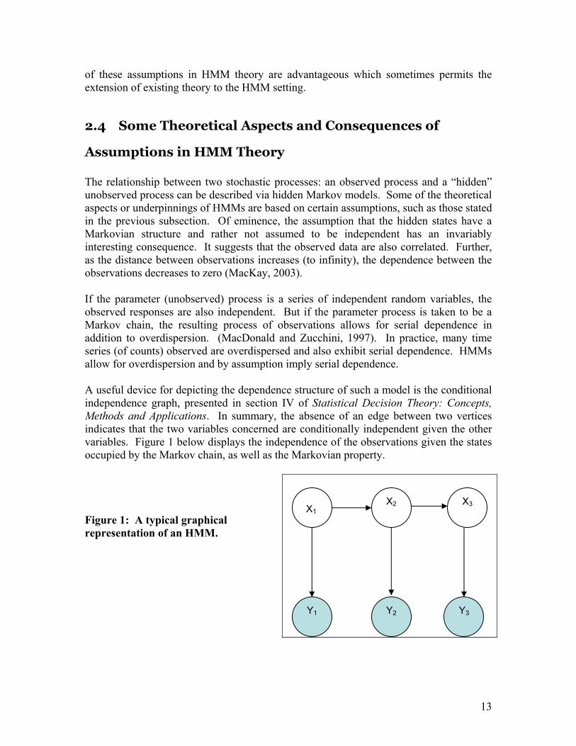
The relationship between two stochastic processes: an observed process and a “hidden” unobserved process can be described via hidden Markov models. Some of the theoretical aspects or underpinnings of HMMs are based on certain assumptions, such as those stated in the previous subsection. Of eminence, the assumption that the hidden states have a Markovian structure and rather not assumed to be independent has an invariably interesting consequence. It suggests that the observed data are also correlated. Further, as the distance between observations increases (to infinity), the dependence between the observations decreases to zero (MacKay, 2003). If the parameter (unobserved) process is a series of independent random variables, the observed responses are also independent. But if the parameter process is taken to be a Markov chain, the resulting process of observations allows for serial dependence in addition to overdispersion. (MacDonald and Zucchini, 1997). In practice, many time series (of counts) observed are overdispersed and also exhibit serial dependence. HMMs allow for overdispersion and by assumption imply serial dependence. A useful device for depicting the dependence structure of such a model is the conditional independence graph, presented in section IV of Statistical Decision Theory: Concepts, Methods and Applications. In summary, the absence of an edge between two vertices indicates that the two variables concerned are conditionally independent given the other variables. Figure 1 below displays the independence of the observations given the states occupied by the Markov chain, as well as the Markovian property. Figure 1: A typical graphical representation of an HMM.

Y3 Y2 Y1

X3 X2 X1

14

Much of the definition of HMMs, thus far, has been provided based on discrete distributions. However, much of the properties can be attributed to a wide range of discrete-valued time series models. In instances where continuous observations are required, continuous conditional distributions can be used (MacDonald and Zucchini, 1997). It has been reported that continuous-time valued hidden Markov models have been applied successfully in applications. An important feature of any time series model is its serial dependence structure. In the theory of normal models, the autocorrelation function reveals this quality. This function is also useful when dealing with discrete-time valued time series models. However, depending on the structure of the process, the autocorrelation function is not the only tool accessible to revealing the serial structure. These correlation properties lead to the central trait which makes HMMs feasible as practical statistical models. The Markovian assumption results in long-range correlations (MacKay, 2003) or serial dependence. This property reveals that the likelihood of even a very long sequence of observations can be computed sufficiently fast to enable parameters to be estimated by direct numerical maximization of the likelihood. Thus, the underlying principle or assumption of the HMMs is that the process can be well characterized as a parametric process, and that the parameters of the stochastic process can be estimated precisely (Rabiner, 1989). Before delving into the computational methods employed for solving HMM problems (in section 4), it is important to describe the various types or variants of hidden Markov models.

2.5 Summary Remarks This section has formally defined hidden Markov models and presented some of the underlying theory. Although much of the formulations have been provided for the discrete case, theoretical arguments were given for continuous and other time series models. These extensions and variants of HMMs are discussed in further detail in the next section. Since the objective of HMMs is to characterize the dynamic structure of the random stochastic process, much of the computational issues are focused on the training and testing of HMMs. These algorithms exist and are explored in detail in section 4.

15

Section 3: Types of Hidden Markov Models There are three basic types of HMMs, differentiated by their method of modeling output probabilities. The observations of the discrete HMM are discrete symbols of a finite alphabet that typically correspond to quantization levels (classes) of a vector quantization codebook. Each state has a discrete probability mass function (PMF) for describing the probability that the state would produce a certain symbol. Much of the discussion, to this point, has considered this discrete case with the mention of the theoretical extensions to other observational forms. This section extends the definition of hidden Markov models to include (semi-)continuous densities and autoregressive models. Furthermore, representation of HMMs and their variants as dynamic Bayesian networks (DBNs) are discussed. HMMs take various forms including ergodic (fully connected) or holding other properties of signals which are desirable for the process being modeled. This section begins with an alternative to the conventional ergodic model.

3.1 Left-Right Model The hidden Markov models defined in section 2 were described as being ergodic. That is that they held the property that every state can be reached from every other state of the model in a finite number of steps. Such ergodic models are fully connected which infers that every state can be reached in a single step. This type of model holds certain advantageous traits such as every ija coefficient is positive which constitute the elements of the state transition probability distribution. However, other types of HMMs have been developed which account for more of the processes attributes than the conventional ergodic model. Such models are more beneficial to a wide range of applications. Of most prominence is the left-right model (also commonly referred to as the Bakis model) (Rabiner, 1989). As the name infers, this model has the underlying assumption that the states proceed from left to right. Thus, the state sequence associated with the model has the property that as time increases the state index increases or remains the same. Processes which have the property of changing over time are readily described by such HMMs. In HMMs of the ergodic form, every ija coefficient is positive; however, in the left-right type of HMMs, the state transition coefficients have the property that

. ,0 ijaij <=

16

This contests that no transitions are allowed to states in which the indices are lower than the current state. Comparatively, the state transition matrix for an ergodic model takes the form

=

ijii

j

j

ergodic

aaa

aaaaaa

A

L

MOMM

L

L

21

22221

11211

,

while the state transition matrix for a left-right model has the form

=−

ij

jrightleft

a

aaaa

A

L

MOM

L

L

000

00

222

1211

.

In the left-right model, the specifications for the state transition coefficients are generally given as

. ,01

Niaa

Ni

NN

<==

Additional constraints are often placed to ensure that large jumps in states do not occur. In general, such a constraints has the form

. ,0 ∆+<= ijaij

For instance, if the model was to ensure that no jumps of more than two states are to incur than ∆ would simply be set to two. The left-right model holds other desirable properties due to the underlying state sequence associated with the model. Since the state sequence begins in state 1 and proceeds right to N, the initial state probabilities take the form

=≠

=.1 ,1 1 ,0

ii

iπ

Left-right type HMMs also have the advantage of being easily represented diagrammatically. This representation will be shown to be more conducive in the latter part of this section. It is important to note that left-right type HMMs and ergodic HMMs are not the only forms of state-space models can be represented. Many other variants of HMMs exist and are discussed extensively in the literature and have been shown to be quite favorable in various applications (Rabiner, 1989; Murphy, 2002).

17

3.2 Continuous and Semi-continuous HMMs In many applications, the observations are continuous processes (or vectors). To this point, the discussion has centered round observations which are discrete and hence characterized by finite discrete symbols. It is possible, in a similar manner, to quantize such continuous responses via codebooks; however, there may be some degradation associated with such quantization. Hence, it is important to provide plausible restrictions to the formulation of continuous HMMs which allow them to be feasible. In contrast to the discrete HMMs, the states of the continuous HMMs each have a mixture of probability density functions (PDFs) to represent the probability of observing certain multi-dimensional continuous data. Since the observations are continuous then the parameters have to be specified for a continuous PDF instead of a discrete PMF. Typically, mixtures of Gaussian (normal) PDFs are used to accurately model the state’s membership in the space of observation vectors. It is usually approximated by a weighted sum of M Gaussian distributions (ℵ). Such a finite mixture of takes the form

∑=

Σℵ=M

1m),,()( jmjmjmj cb µOO

where,

. statein component mixture for thematrix covariance

,rmean vecto

, statein mixture for thet coefficien mixture

jm

jmc

thjm

jm

thjm

=Σ

=

=

µ

Although ℵ is not confined to being a Gaussian distribution it most typically is. However, it should be log-concave or elliptically symmetric (Rabiner, 1989). Moreover, the mixture coefficients should satisfy the following stochastic constraints,

MmNjc jm ≤≤≤≤≥ 1 ,1 ,0

and

∑=

≤≤=M

mjm Njc

11 ,1 .

Then, for an HMM with continuous densities, ),,,,( πλ jmjmjmcA Σµ= . A modification of continuous HMMs is semi-continuous HMMs. The semi-continuous HMM is a hybrid of the discrete and continuous case. Like the discrete HMM, the

18

observation vectors are quantized into one of a finite set of classes, reducing the number of free parameters. However, like the continuous HMM, the observation classes are modeled by a multivariate Gaussian PDF, removing the distortion due to quantization and effectively modeling the variance of an observation class. This formulation is similar to a continuous HMM with parameter tying in which states are forced to share the same PDFs. Initially formed by clustering the sample data, the classes are re-estimated with the HMM parameters to form an integrated model. The concept of parameter tying is based on an equivalence relation between HMM parameters in different states. This reduces the number of independent parameters in the model and simplifies parameter estimation (Rabiner, 1989). Such HMMs are used in applications where the densities for two or more states are considered to be the same. An interesting HMM variant is one in which the observations are associated with transitions which produce no output. That is, it moves from one state to another without an observed response. Such transitions are called null transitions. These and other variants find purpose in a wide range of applicants. The reader is deferred to Murphy (2003) for a discussion of HMMs and their variant structures.

3.3 Autoregressive (AR) HMMs Discrete and continuous HMMs or even their hybrids form the two of the basic types of HMMs based on the output distributions. Another class of HMMs is that which draws upon real-world processes which are autoregressive. In such models, the observation vectors are drawn from an autoregressive process. In simplicity, an autoregressive (AR) model is in time series analysis where the observation is postulated to be a linear function of previous values of the series (Everitt, 2002). A first-order autoregressive model has the form

ttt eaxx += −1

where tx is an observation at time t, a is a parameter of the model and te is a random disturbance of the model. A p-order model takes the form

tptpttt exaxaxax ++++= −−− ...2211

which includes the p parameters of a. Now consider an observation vector O with components ),...,,,( 1210 −kxxxx . Assuming a Gaussian distribution, the observation vector is a p-order Gaussian autoregressive and the components of the observation vector have the following relationship (Rabiner, 1989)

∑=

− +−=p

ikikik ea

1OO

19

where 1,...,2,1,0 , −= Kkek are Gaussian independent identically distributed random variables with zero mean and variance 2σ , and ia are the autoregression coefficients. The density function for O is approximated by

−= − ),(

21exp)2()( 2

2/2 aOO δσ

πσ Kf

where

].,...,,1[

)()(2)0()0()(

21

1

p

p

iaa

aaa

irirrr

=′

+= ∑=

a

aO,δ

Recall in section 2.3 that the importance of the serial dependence structure in time series models is revealed via the autocorrelation function. See MacDonald and Zucchini (1997) for a full derivation of the autocorrelation function and many of the corresponding theoretical aspects. It should be noted that the functions )(ir and )(ira are the autocorrelation functions of the observed samples and the autoregressive coefficients, respectively. These autocorrelation functions take the following form

∑

∑−

=+

−−

=+

≤≤==

≤≤=

ip

ninna

iK

ninn

piaaair

pixxir

00

1

0

.1 ),1( )(

,0 )(

To define an (Gaussian) autoregressive HMM, the elements of the emission matrix assume a mixture density of the form

∑=

=M

mjmjmj bcb

1)()( OO

where )(Ojmb is the density with autoregression vector jma

−

=

−

)(2

exp2)(2/

jm

K

jmK

Kb aO,O δπ .

The standard conditional independence assumption in HMMs (described earlier) is quite strong and which can be relaxed in its autoregressive form. It reduces the effect of the hidden nodes “bottleneck” by allowing the previous observation to help predict the current observation. The consequence is that it results in models with higher likelihood (Murphy, 2002). Generalized autoregressive HMMs also exist which allow for non-

20

linear dependencies between the observable responses. These models find value in their applications to speech processing, finance and various areas of engineering.

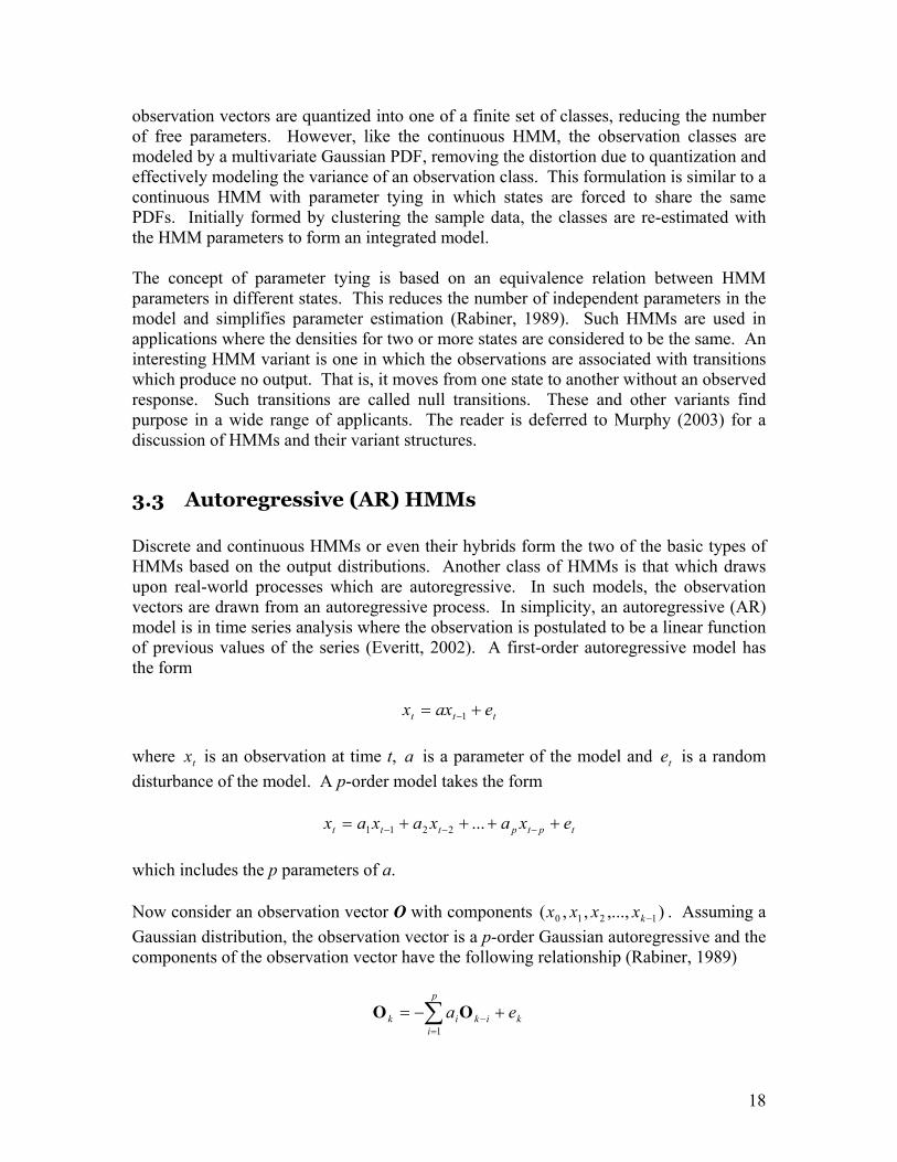
3.4 Representation of HMMs This section has focused on HMMs and their variants with little discussion on the versatility these models demonstrate through their representational forms. In many applications of HMMs, the attempt is to explain the dynamic structure of the random (stochastic) process. Representation of HMMs as dynamic Bayesian networks (DBNs) is one novel approach. Thus, the objective is to model a dynamic system rather than a networks change over time. See Murphy (2002) for a discussion of DBNs which change their structure over time. The reader is also deferred to section IV of Statistical Decision Theory: Concepts, Methods and Applications for a formal discussion on probabilistic graphical models in sequential methods. Consider a discrete stochastic process where K,, 21 ZZ are random variables (r.v.) and that ),,( tttt YXUZ = can be partitioned into its input, hidden, and output variables of a hidden Markov model. Recall that each node has a conditional probability distribution (CPD) which defines the structure. An assumption in HMMs is that { }tZ is time-homogeneous. That is, the assumption that the parameters of the CPDs are time- invariant. Murphy (2002) and Jordan (1999) argue that if the parameters can change, then they can be treated as r.v.s. Alternatively, if there are a finite number of parameter values, then a hidden variable can be used to select a suitable set of random variables. Representing HMMs and their variants as probabilistic graphical models has the advantage to create extensions and modifications on the basic theme. Below are a series of HMMs and their variants (as discussed in this section).

Figure 2: An HMM in which the parameters are explicitly shown.

Y3 Y2 Y1

X3 X2 X1

B

A π

21

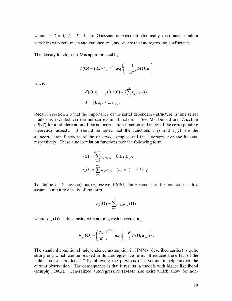
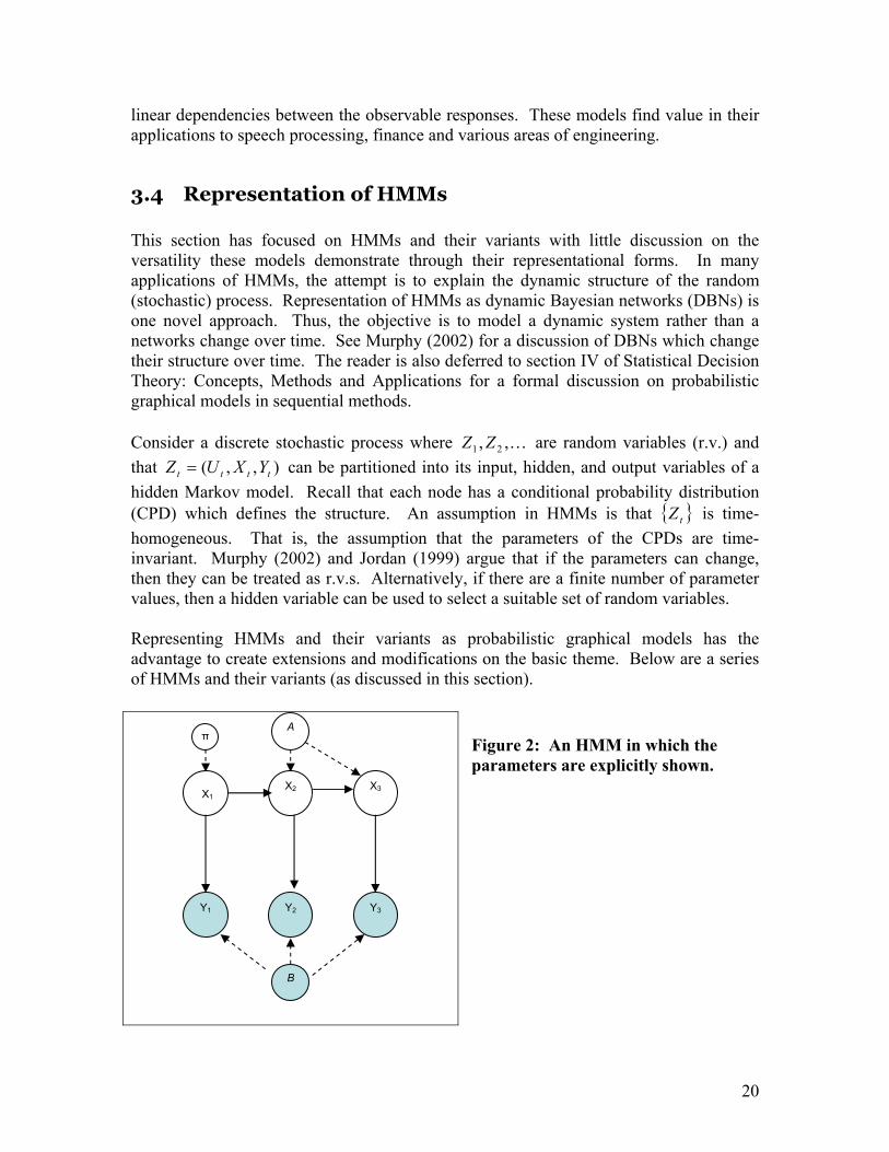
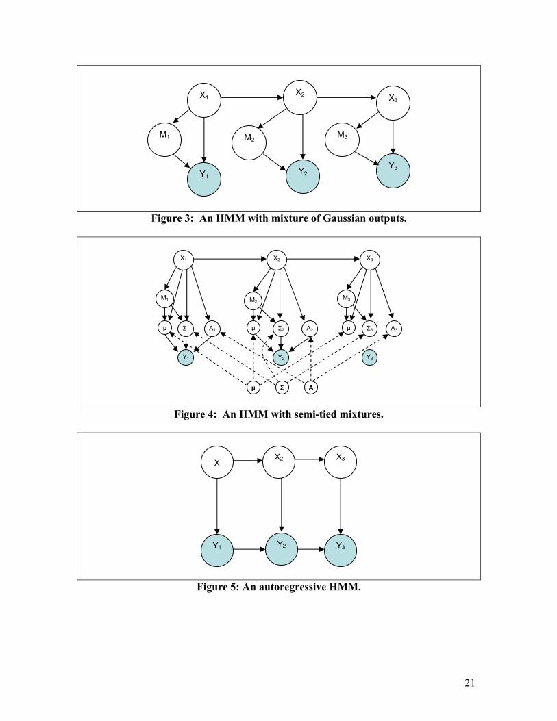
Figure 3: An HMM with mixture of Gaussian outputs.

Figure 4: An HMM with semi-tied mixtures.

Figure 5: An autoregressive HMM.

Y3 Y2 Y1

X3 X2 X

X1 X2 X3

M1 M2 M3

µ µ µΣ1 A1 Σ2 A2 Σ3 A3

Y1 Y2 Y3

AΣµ

M1 M2

X1

Y1 Y2

X2

M3

Y3

X3

22

3.5 Other Remarks As demonstrated in this section, hidden Markov models have been designed for various output probabilities. Furthermore, extensions and modification of HMMs have also been developed for a wide variety of applications. At the beginning of this section, the left-right model was introduced and subsequently, imposed constraints on the state transition matrix. The transient nature of the states within the model only allows a small number of observations for any state (Rabiner, 1989); thus, to make the parameter estimates reliable, multiple processes are suggested. MacKay (2003) explores multiple processes in HMMs with random effects building on the ideas of generalized linear mixed models. AR-HMMs for multivariate time series have also been discussed in MacDonald and Zucchini (1997) for count processes. However, there is still deficiency in this area which is still needed to be filled.

23

Section 4: Computational Methods for HMMs The goal or underlying postulation of hidden Markov models is that the observed response can be characterized as a parametric random process, and that such parameters of the stochastic process can be estimated precisely. The previous sections described the various formulations of HMMs; however, their application is based on three fundamental problems. These problems are most commonly referred to as the evaluation problem, the decoding problem, and the learning problem. In this section, these three fundamental problems for HMMs are stipulated in their probabilistic context and formal mathematical solutions for each problem are presented.

4.1 The Three Fundamental Problems for HMMs A discrete-time or discrete-space dynamical system governed by a Markov chain emits a sequence of observable outputs where one output (observation) for each state is in trajectory of such states. From the observable sequence of output, the most dynamical system can be inferred. The result is a model for the underlying process. Alternatively, given a sequence of outputs, the most likely sequence of states can be inferred. Hidden Markov models are used in a wide variety of applications. The motivation for using these models lays in its assumed ability to divulge the dynamical structure of real-world processes. Thus, given an HMM there are three basic problems of interest. The Evaluation Problem: Given an HMM λ and a sequence of observations TOOOO ,...,, 21= , what is the probability that the observations are generated by the model )|( λOP ? Thus, the objective of this problem is to compute the probability that the observed sequence was produced by the model. Since the objective is to determine whether a given model matches an observation sequence, this conceptualization can be extended to determine model selection. The Decoding Problem: Given an HMM λ and a sequence of observations TOOOO ,...,, 21= , what is the most likely state sequence in the model that produced the observations? Thus, the objective of the decoding problem is to unveil or uncover the hidden states. Since the objective is to learn about the topological structure of the model, optimality criteria are usually used to decode the state sequence.

24

The Learning Problem: Given an HMM λ and a sequence of observations TOOOO ,...,, 21= , how should the model parameters be adjusted in order to maximize the probability that observations are generated by the model )|( λOP ? This latter problem is central to many applications of HMMs as it allows for an optimal adaptation of the model parameter to an observation sequence. Such an observation sequence is referred to as a training set as it is used to train the HMM. Thus, the objective of the learning problem is to optimize the model parameters so to best describe the observation process. The computational process of solving these three basic problems assumes that a codebook with M unique feature vectors have been coded; hence each observation is the index of the feature vector closest (in some distance sense) to the actual state. Thus, for every object of interest (albeit characters, words, textures, tasks, “states” of a system), there is a training sequence consisting of a number of repetitions of sequences of codebook indices of the “state”. Then the first task is to build individual object models or state-space models which are accomplished by estimating model parameters for each object. Then to understand the dynamic structure of the process, the solution to the decoding problem must be implemented. Since the ultimate goal is to refine the model so it will recognize an unknown observation sequence. The evaluation problem can be used to determine whether the observed pattern is recognized based on likelihood methods.

4.2 The Evaluation Problem The evaluation problem is determining the probability of the observation sequence given the model. Using simple probabilistic arguments, given the model λ and an observation sequence, )|( λOP can be determined. See Rabiner (1989). But this calculation requires a large number of operations in the order of TN , since there are N possible states. Even if the length of the sequence of T is quite moderate, this would be computationally unfeasible. Fortunately, a more feasible and efficient algorithm exists – the forward-backward procedure. This procedure makes use of an auxiliary variable )(itα called the forward variable. The forward variable is defined as the probability of the partial observation sequence,

tOOO ,...,, 21 , until it terminates at state i. This can be mathematically stated as

)|,,...,,()( 21 λα ittt SqOOOPi == .

Recursively, the following relationship holds

NjTtObaij tj

N

iijtt ≤≤−≤≤

= +

=+ ∑ 1 ,11 ),()()( 1

11 αα

where

25

NiObi ii ≤≤= 1 ),()( 11 πα .

Using this recursion, )(iTα for Ni ≤≤1 can be calculated and the required probability can be determined as

∑=

=N

iT iOP

1

)()|( αλ .

In summary, the first step is to initialize the forward probabilities as the joint probabilities of the state iS and the initial observation 1O . The next step is the recursion formula which determines the probability of the joint event that tOOO ,...,, 21 is observed and state

jS is reached a time t + 1. Summing these probabilities and multiplying them by the probability )( 1+tj Ob , )(1 jt+α is obtained. Finally, the sum of the terminal forward variables gives )|( λOP . This forward probability calculation is based on the lattice structure (Ripley, 1987) which resides in the understanding that the all the possible state sequences will remerge in to the N nodes. This algorithm requires TN 2 calculations and is less computationally intensive then direct calculations. In a similar manner, the backward variable can be defined as the probability of the partial observation sequence Ttt OOO ,...,, 21 ++ , given that the current state is i. Mathematically, this is stated as

)|,,...,,()( 21 λβ itTttt SqOOOPi == ++ .

As in the case of )(itα , there is a recursive relationship which can be used to calculate )(itβ efficiently as follows

∑ ≤≤−−=++ NiTTtjObai ttjijt 1 ,1,...,2,1 ),()()( 11 ββ

where

NiiT ≤≤= 1 ,1)(β . Further, it can be seen that

)|,()()( λβα ittt SqPii == O . Therefore, the )|( λOP can be computed by using both the forward and backward variables as follows

26

∑∑==

===N

itt

N

iit iiSqOPOP

11

)()()|,()|( βαλλ .

This latter calculation of the backward variable is very useful for solving the decoding and learning problem.

4.3 The Decoding Problem and Pattern Recognition The goal of the decoding problem is to determine the dynamical structure of the observed process. This involves the construction of a pattern recognition system. Performing a recognition algorithm or decoding procedure is a simpler process than the latter problem of training an HMM. However, it is a mathematically rigorous filed with the purpose of classifying objects into one of a number of classes. The construction of a pattern recognition system involves learning from a set of example patterns and has two forms. A supervised pattern recognition assumes that the classes of the example patterns are known. The correct classification of an individual pattern is used to evaluate the performance of the system and the feedback system allows the system to iteratively improve itself. If the classes are not known, the task is more difficult as it must also define a classification procedure. This latter type of system is called unsupervised pattern recognition. The actual pattern recognition process is performed in two phases, the first of which is feature extraction, where the observation x of a pattern is transformed into a vector y, whose components are called features. These features may be physical attributes of the problem or mathematical constructs for reducing the dimensionality of the observations. The second phase is the classification of the feature vectors. A classifier partitions the feature space of y into disjoint regions, each corresponding to a pattern class. A classifier for a supervised recognition system is relatively simple since the classes are known; however, if the classes are unknown then cluster analysis methods are required. The classification redeems model as the system recognizes the phenomenon. Statistically, the solution to the decoding problem depends on the way “the most likely sequence” is defined. Although there are several optimality criteria available, the most common is based on dynamic programming methods (explained in section V of Statistical Decision Theory: Concepts, Methods and Applications), and is called the Viterbi algorithm. This algorithm facilitates the single best state sequence with the maximum likelihood. Much like the forward-backward algorithm, it makes use of an auxiliary variable

)|...,...(max)( 2121,...,, 121

λδ titqqqt OOOSqqqPit

==−

which gives the highest probability that the partial observation sequence and state sequence at time t can have. Thus, the following recursive relationship holds

27

11 ,1 ),(])(max[)( 111 −≤≤≤≤⋅= +≤≤+ TtNiObaij tjijtNit δδ

where,

NiObi ii ≤≤= 1 ),()( 11 πδ . So the procedure to finding the most likely state sequence starts from calculation of

)( jTδ , Nj ≤≤1 using the recursion formula, while always keeping a pointer to the optimal state. Finally, the state j* is found by

)(maxarg*1

jj TNj

δ≤≤

=

and starting from this state, the sequence of states is back-tracked as the pointer indicates, giving the required set of states. Thus, this algorithm is a search procedure whose nodes represent states in an HMM, as discussed in section 3.4.

4.4 The Learning Problem Generally, the learning problem is determining how to adjust the HMM parameters, so that the given set of observations (the training set) is represented by the model in the best way for the intended application. Thus, the learning process can be different from application to application. In other words there may be several optimization criteria for learning, out of which a suitable one is selected depending on the application. There are two main optimization criteria found in the literature; Maximum Likelihood (ML) and Maximum Mutual Information (MMI). A solution to the learning problem under the ML criteria is presented and brief disucussion to the MMI criteria is given below. In ML, the objective is to maximize the probability of a given sequence of observations, given the HMM ),,( πλ BA= . This probability is the total likelihood of the observations and can be expressed mathematically as )|( λOPL = . Since there is no analytic method to solve for the model ),,( πλ BA= , which maximizes )|( λOPL = , an iterative procedure can be used to choose model parameters such that it is locally maximized such as the Baum-Welch method (equivalently known as the expectation-modification (EM) method) or a gradient based method. This section focuses on the Baum-Welch approach. In many regards the Baum-Welch algorithm is an extension of the Forward-Backward algorithm. Similar to the forward and backward variables, this procedure requires the use of two more auxiliary variables which can be expressed in terms of the forward and backward auxiliary variables. The first defines the probability of being in state iS at time t and at state jS at time t+1 and can be expressed as

28

.)|(

),,,(

),|,(),(

1

1

λλ

λξ

OPOSqSqP

OSqSqPji

jtit

jtitt

===

===

+

+

Re-expressing this in terms of the forward and backward variables gives

∑∑= =

++

++= N

i

N

jttjijt

ttjijtt

jObai

jObaiji

1 111

11

)()()(

)()()(),(

βα

βαξ .

The second auxiliary variable used in the Baum-Welch algroithm is the a posteriori probability, ),|()( λγ OSqPi itt == , which is the probability of being in state iS given the observation sequence and model. Re-expressing this variable in terms of the forward and backward variables gives

∑=

= N

itt

ttt

ii

iii

1)()(

)()()(

βα

βαγ .

Thus, the relationship between )(itγ and ),( jitξ is

∑=

=N

jtt jii

1),()( ξγ .

Summing )(itγ and ),( jitξ over t from t=1 to t=T-1 can be easily interpreted as the expected number of transitions from state iS and the expected number of transitions from state iS to jS . Now, having defined all of the auxliary variables, the Baumm-Welch learning process can be described where the parameters of the HMM are updated such that )|( λOP is maximized. Assuming an initial model ),,( πλ BA= , the forward and backward variables α and β can be calculated using the previously described recursion formula. Subsequently, the auxiliary variables γ and ξ can be calculated using their corresponding recursion methods. The next step is to update the HMM parameters according to the re-estimation formulas given below (for the discrete case):

29

state from ns transitioofnumber expected state to state from ns transitioofnumber expected

11 ,)(

),(

1

1

1

1

i

ji

T

tt

T

tt

ij

SSS

NjN, ii

jia

=

≤≤≤≤=

∑

∑−

=

−

=

γ

ξ

and

statein timesofnumber expected symbol observing and statein timesofnumber expected

11 ,)(

)(

)(

1

..1

j

kj

T

tt

vOts

T

tt

j

SvS

NjN, ii

i

kb kt

=

≤≤≤≤=

∑

∑

=

==

γ

γ

and finally

1 at time statein times)of(number frequency expected )(1

===

tSi

i

i γπ.

These re-estimation formulas can also be given for the continuous case (see Rabiner, 1989) and for autoregressive models (see MacDonald and Zucchini, 1997). Iteratively using λ and repeating the re-estimation calculation, the probability of the observation sequence obtained from the model is being improved. The final result is the maximum likelihood estimate of the HMM. An advantage to the Baum-Welch algorithm is that it converges to a critical point – guaranteed convergence. Another popular approach in achieving ML, is using gradient based methods which can be determined with resepct to transition probabilities or with respect to observation (emission) probabilities. This approach can also be extended to the other optimization criterion Maximum Mutual Information (MMI). The goal in ML was to optimize an HMM one at a time (for a particular class). This minimizes the discrimination ability which is critical to pattern recognition. Thus, Thus the ML learning procedure gives a poor discrimination ability to the HMM system, especially when the estimated parameters (in the training phase) of the HMM system do not match with the speech inputs used in the recognition phase. These types of mismatches can arise due to two reasons. One is that the training and recognition data have considerably different statistical properties, and the other is the difficulties of obtaining reliable parameter estimates in the training. The MMI criterion considers HMMs of all the classes simultaneously during training. Parameters of the correct model are updated to enhance it's contribution to the observations, while parameters of the alternative models are

30

updated to reduce their contributions. Both criteria pose advantages and are appropriate in different applications.

4.5 Other Remarks Implementation of HMM algorithms gives rise to several computational issues including initial parameter estimates, missing values and choice model size and type. These issues are not discussed further in this paper and the reader is deferred to (Rabiner, 1989; MacDonald and Zucchini, 1997; and MacKay, 2003). However, critical to HMM problems is the concept of classification. Moreover, since a model is developed for each class, cluster analysis plays a critical role in pattern recognition. Clustering is the process of constructing a classifier for unsupervised pattern recognition. The problem is not only to classify the given data but to simultaneously define the classes. Generally, clusters are groups of similar points according to some measure of similarity defined as proximity measured by a distance function, such as the Euclidian distance or the Mahalanbis square-distance, of feature vectors in the state-space. As mentioned earlier, these clusters may have a physical characterization or a mathematical criterion. In signal processing, vector quantization (clustering using Euclidean distance) is used and the clusters of a classifier are called the quantization levels of a VQ code book. The distance of each sample to the mean of its enclosing cluster is no longer a measure of similarity but rather a measure of distortion. Thus, the goal is to determine the set of quantization levels that minimizes the average distance over all samples. However, this minimal average is intractable (Ripley, 1989). Nonetheless, given the number of k-clusters, convergence to a local minimum can be achieved through a K-means algorithm. Another computational approach or issue is that of multidimensional scaling. Unlike clustering methods which use the observations and a dissimilarity matrix, multidimensional scaling (MDS) techniques seek to find a low dimensional coordinate system to represent the k objects using a proximity matrix usually without observing the observation vectors. Given perceptions or judgments regarding the objects, a low dimensional space to represent the judgments is constructed. This provides another classifying technique. There are various other cluster analysis approaches. However, it is important to apply the appropriate classifying method to the appropriate application.

31

Section 5: HMMs for EMG Pattern Recognition Work-related musculoskeletal disorders (WMSDs) may be attributed to several possible risk factors which can be measured in a variety of capacities. Electromyographical (EMG) signals of the shoulder and forearm muscles have been used to examine relationships between worker-workstation interactions for different tasks. This section explores the use of EMG signals as a source of data which may be appropriately modeled by HMMs. Various types of HMMs and corresponding algorithmic approaches are discussed as a means of EMG pattern recognition. Some preliminary results also demonstrate the achievability of the approach. A proposed framework is given as an extension of existing methodology to assert the use of HMMs and its variants as feasible tools for EMG pattern recognition.

5.1 Rationale/Background Repetitive tasks and workstation configuration are two of many contributing factors to work-related musculoskeletal disorders (WMSDs). Although there is no clear defining measure of factors which are considered risk, there are several techniques which have been studied and provide constructive information. Different tasks may also exhibit unique characteristics which may be potentially more hazardous. Non-optimal positioning of work equipment may also pose as an unfavorable constraint. Posture measures have also been associated with WMSDs (Gerr et. al., 2002); however, such physical attributes may vary accordingly with workstation configurations, tasks performance, and individual behavioral patterns. A more novel approach has been to use electromyographical (EMG) signals to monitor muscle load for different tasks. Modeling exposure measures of WMSDs has predominantly focused on simple regression methods and generalized linear methods. These approaches, although useful in identifying differences in subgroups, provide little information on the dynamic structure of the physical processes (such as postures). Alternatively, Vasko et. al. (2000) proposed an application of hidden Markov model topology estimation to repetitive lifting data to describe the dynamic structure of posture (angle) measures. Their sample was composed of three groups of patients: low back pain pre-treatment, low back pain post- treatment, and a control group with no low back pain. The HMM approach revealed different topology estimates for patients with low back pain versus patients without low back pain. However, there was no dynamic structural difference between the two types

32

of low back pain groups. This provides evidence that posture measures can be successfully modeled using HMM-based pattern recognition methods. Modeling EMG signals provide the advantage of not only taking into account the level of muscle activity but also the duration and intensity of each muscle contraction. Similar to other physical measures, generalized linear models have been primarily used to examine differences in EMG performance for different tasks or groups of subjects. Since different physical motions impose different modes of muscle activation, distinct EMG patterns are generated. Literature in the discrimination (or recognition) of EMG patterns is minimal; however, various techniques have been proposed. Of primary interest has been the use of autoregressive (AR) models to represent an EMG signal (Graupe et. al., 1978) and a multi-dimensional AR models to model multi-channel EMG signals (Tsuji et. al., 1987). More recently, neural networks have been employed to model the dynamic structure of the physical process in the field of prosthetic control (Bu et. al., 2003; Soares et. al., 2003). Both used neural networks as an EMG pattern recognition method and demonstrated successful discrimination of forearm motions. The purpose of this paper is to demonstrate the feasibility and performance of HMMs as a novel device in determining the dynamic structure of such physical (stochastic) processes as EMG. This section begins by describing EMG signal processing and extends itself as a source of data which can be precisely modeled by HMMs. A discussion on the use of HMMs as a model-based indicator of WMSDs is explored via classification methods. Results lead to a presentation of a theoretical framework of an EMG pattern recognition method based on HMM algorithms. Guidelines for future work conclude this paper.

5.2 EMG Signal Processing Electromyographical (EMG) signals are electrical manifestations of the neuromuscular activation associated with contracting a muscle (Cram, 1998). This signal process is exceedingly complicated by extraneous factors such as muscle fatigue, sweat and changes in electrode location. Thus, the process of detecting an EMG signal is not trivial as it is superceded by impure signals that come from various difference sources of noise. Other factors related to the electrode-skin interface may also impede the detection of an EMG signal. The distance between pairs of electrodes and the region where must be carefully considered in experimental procedures used in this work. Filters also exist which can remove unwanted components of the EMG signal. EMG signals are detected by surface electrodes and filtered before data acquisition. In order to process the correct portion of the signal, the start point of the EMG activity needs to be determined so that a portion can be extracted (forming a feature). The resulting EMG signal is regarded as a stochastic process which is formulated as the sum of the “spike potential” generated in the motor units. Thus, the goal then becomes to characterize this dynamic structure by classifying the EMG pattern. This paper proposes the use of HMM-based classifiers to accomplish this task.

33

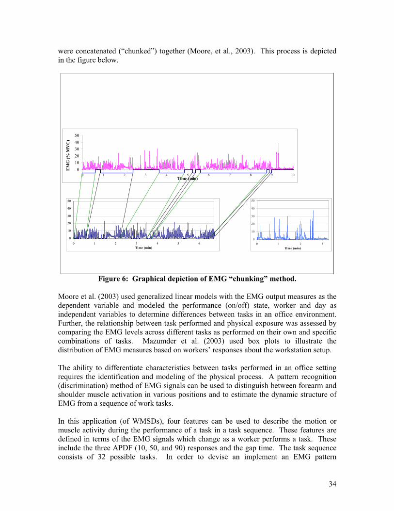
5.3 Methods and Analysis A study was conducted to examine the relationships between measures of workstation-worker interaction and EMG signals of the shoulder and forearm muscles for different tasks. It was hypothesized that a higher level of muscle activity would be identified for workers whose equipment was considered to be in a non-optimal position. A sample of 41 workers was recruited from a workplace study at a large urban newspaper: (71% female), they had a mean of 41 years (sd=9.6), a mean height of 168cm (sd=10.3) and a mean weight of 74kg (sd=19). Various methods were used to obtain information on work exposures to WMSDs including the administration of a questionnaire and task diary, direct observation, video recording and various physical exposures such as dimension and posture measures as well as EMG data. Of particular interest to this paper is the EMG data collected on these workers. Electromyographical signals were recorded bilaterally from Extensor Carpi Radialis Brevis (ECRB) and trapezius (shoulder and forearm muscles) on two different days for a two hour period each day. The EMG was recorded simultaneously with the videotape. Root Mean Square (RMS) EMG was collected at 10 Hz using a commercially available portable system (ME3000P8, MEGA electronics, Finland, CMRR 110 dB, 15-500 Hz). It was collected using silver/silver-chloride disposable electrodes at a 2 cm spacing. For ECRB, the electrodes were placed one third of the distance from the lateral epicondyle to the radial styloid. For trapezius, the electrodes were placed midway between C7 and the Acromion. The EMG was started in view of the camera and was later marked using a switch provided by the equipment to allow for synchronization of the EMG video. EMG measures were calibrated both to Maximum Voluntary Contraction (MVC) and to Relative Voluntary Exertion (RVE). For trapezius, the MVC was achieved by having participants pull maximally against straps that were fixed to the floor and looped over their elbows while they stood with both shoulders abducted 90 degrees. For the ECRB, MVC was recorded while the participants simultaneously performed a maximal grasp while extending their wrist. For the RVE, they supported a 5 Kg load hung by a strap over their joints. Tests were also performed to confirm signal quality and quiet level. The EMG signal was analyzed using two methods commonly used for workplace analysis: APDF-Amplitude Probability Distribution Function (Jonsson, 1982) and a Gaps Analysis (Veiersted et al., 1990). The APDF allows for a cumulative summary of all the EMG levels used throughout a specified time period, and is usually summarized using three points – the static level (10th %ile), the median (or dynamic) level (50th %ile), and the peak level (90th %ile). The gap analysis calculates the portion of the period of interest in which the muscle gets rest for at least 0.2 seconds. The periods of interest consisted of the EMG corresponding to the performance of a specific task or group of tasks. This was achieved using custom software which linked the video analysis with the EMG recordings in time. Once linked, all samples of EMG corresponding to a particular task

34

were concatenated (“chunked”) together (Moore, et al., 2003). This process is depicted in the figure below.

0

10

20

30

40

50

0 1 2 3Time (min)

0

10

20

30

40

50

0 1 2 3 4 5 6Time (min)

-100

1020304050

0 1 2 3 4 5 6 7 8 9 10Time (min)

EM

G (%

MV

C)

Figure 6: Graphical depiction of EMG “chunking” method.

Moore et al. (2003) used generalized linear models with the EMG output measures as the dependent variable and modeled the performance (on/off) state, worker and day as independent variables to determine differences between tasks in an office environment. Further, the relationship between task performed and physical exposure was assessed by comparing the EMG levels across different tasks as performed on their own and specific combinations of tasks. Mazumder et al. (2003) used box plots to illustrate the distribution of EMG measures based on workers’ responses about the workstation setup. The ability to differentiate characteristics between tasks performed in an office setting requires the identification and modeling of the physical process. A pattern recognition (discrimination) method of EMG signals can be used to distinguish between forearm and shoulder muscle activation in various positions and to estimate the dynamic structure of EMG from a sequence of work tasks. In this application (of WMSDs), four features can be used to describe the motion or muscle activity during the performance of a task in a task sequence. These features are defined in terms of the EMG signals which change as a worker performs a task. These include the three APDF (10, 50, and 90) responses and the gap time. The task sequence consists of 32 possible tasks. In order to devise an implement an EMG pattern

35

recognition method via HMM algorithms, however, a codebook or some form of classification method must be devised in order to determine the number of possible classes. There are two (most eminent) ways in which from a physical judgment this can be devised. Workers can be classified into two groups: optimal workstation setup versus non-optimal workstation setup. Or workers can be classified according to symptoms (pain or discomfort) of WMSDs to determine differences in the topological structure of each of these groups. Both k-means clustering and multidimensional scaling approaches are explored in order to create a codebook.

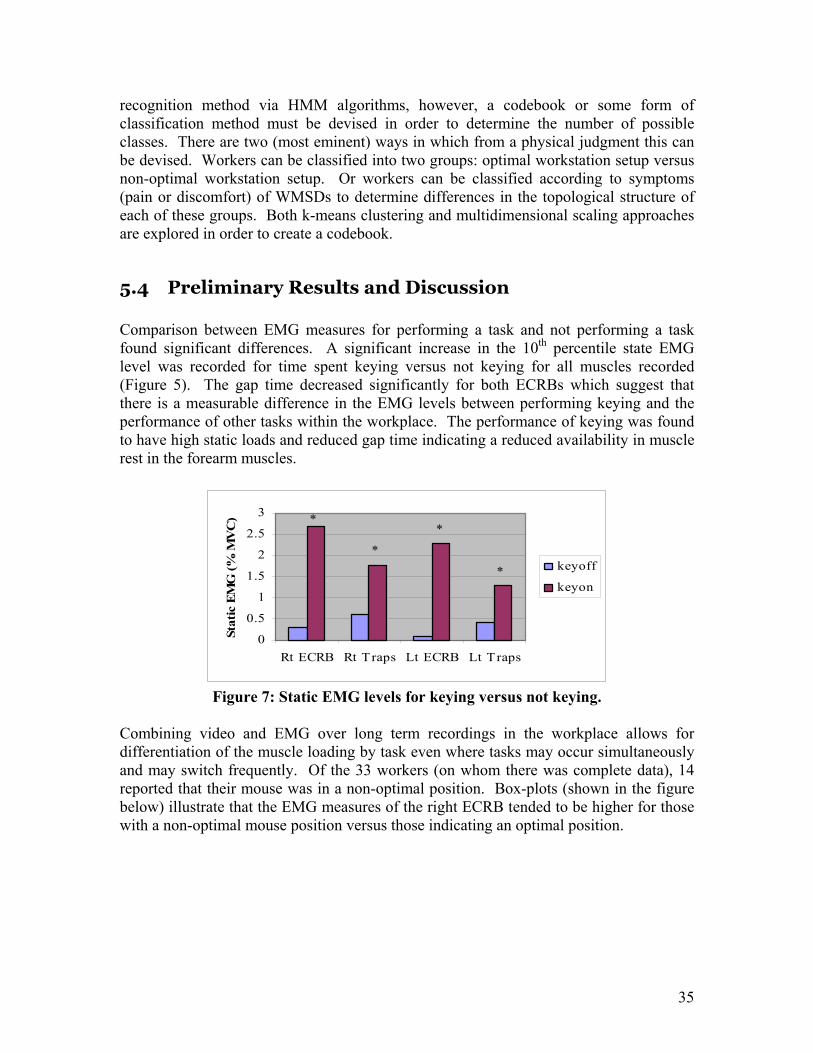
5.4 Preliminary Results and Discussion Comparison between EMG measures for performing a task and not performing a task found significant differences. A significant increase in the 10th percentile state EMG level was recorded for time spent keying versus not keying for all muscles recorded (Figure 5). The gap time decreased significantly for both ECRBs which suggest that there is a measurable difference in the EMG levels between performing keying and the performance of other tasks within the workplace. The performance of keying was found to have high static loads and reduced gap time indicating a reduced availability in muscle rest in the forearm muscles.

0

0.5

1

1.5

2

2.5

3

Rt ECRB Rt Traps Lt ECRB Lt Traps

Stat

ic E

MG

(% M

VC

)

keyoff

keyon

*

*

*

*

Figure 7: Static EMG levels for keying versus not keying.

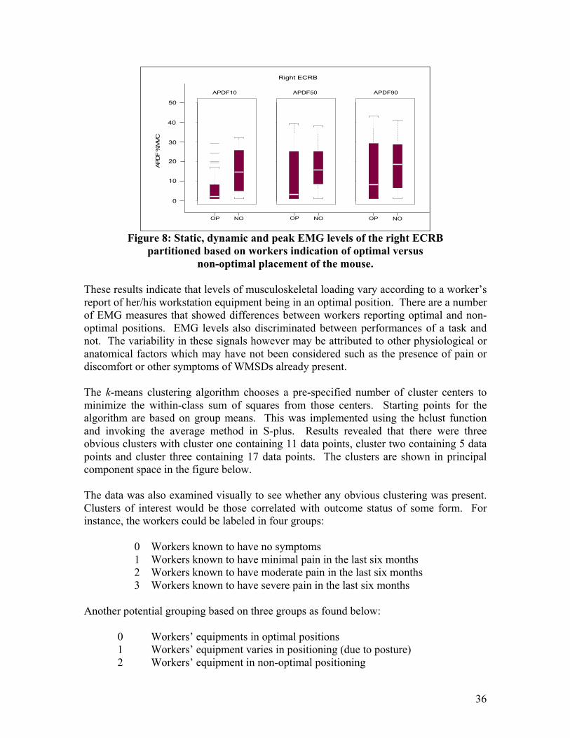
Combining video and EMG over long term recordings in the workplace allows for differentiation of the muscle loading by task even where tasks may occur simultaneously and may switch frequently. Of the 33 workers (on whom there was complete data), 14 reported that their mouse was in a non-optimal position. Box-plots (shown in the figure below) illustrate that the EMG measures of the right ECRB tended to be higher for those with a non-optimal mouse position versus those indicating an optimal position.

36

010

2030

4050

1 2

010

2030

4050

1 2

010

2030

4050

1 2

0

10

20

30

40

50

APDF10 APDF50 APDF90

Right ECRB

OP NO OP NO OP NO

APDF

%M

VC

Figure 8: Static, dynamic and peak EMG levels of the right ECRB

partitioned based on workers indication of optimal versus non-optimal placement of the mouse.

These results indicate that levels of musculoskeletal loading vary according to a worker’s report of her/his workstation equipment being in an optimal position. There are a number of EMG measures that showed differences between workers reporting optimal and non-optimal positions. EMG levels also discriminated between performances of a task and not. The variability in these signals however may be attributed to other physiological or anatomical factors which may have not been considered such as the presence of pain or discomfort or other symptoms of WMSDs already present. The k-means clustering algorithm chooses a pre-specified number of cluster centers to minimize the within-class sum of squares from those centers. Starting points for the algorithm are based on group means. This was implemented using the hclust function and invoking the average method in S-plus. Results revealed that there were three obvious clusters with cluster one containing 11 data points, cluster two containing 5 data points and cluster three containing 17 data points. The clusters are shown in principal component space in the figure below. The data was also examined visually to see whether any obvious clustering was present. Clusters of interest would be those correlated with outcome status of some form. For instance, the workers could be labeled in four groups:

0 Workers known to have no symptoms 1 Workers known to have minimal pain in the last six months 2 Workers known to have moderate pain in the last six months 3 Workers known to have severe pain in the last six months

Another potential grouping based on three groups as found below:

0 Workers’ equipments in optimal positions 1 Workers’ equipment varies in positioning (due to posture) 2 Workers’ equipment in non-optimal positioning

37

Thus, there are a variety of possible descriptions which this data can be classified into. For experimental purposes, a backward propagation method (a variation of the forward-backward algorithm) used in neural networks employed in S-plus was employed to determine the dynamic structure for two different workers. One worker indicated having a keyboard in a non-optimal position while the other claimed having a keyboard in an optimal position. Each modeled demonstrated structural differences for some of the features; however, static levels did not appear to be very different across subjects.

5.5 Proposed Framework for an EMG Pattern Recognition Method The proposed discrimination method is an extension and modification of existing work in the field. The structure of the method consists of three parts in sequence: (1) EMG signal processing, (2) HMM-based learning algorithm, and (3) a discrimination rule. The first step of which involves signal processing as it extracts the feature patterns. This can be done quite attractively by the method previously employed. And thus, there are four measures which describe the structure of the physical process: the 10th, 50th, and 90th percentile of the APDF and the gap time measure. The next step is the crux of the method as it employs HMM algorithms for pattern discrimination. Consider a dynamic probabilistic model where there are K classes in this model and each class k }),...,1{( Kk ∈ is composed of N states. Suppose that for the given observation sequence (a time series) TxxxO ,...,, 21= , at any time tx must occur from one state iS to state jS of class k in the model. Thus, the a posteriori probability for class k, is calculated as

∑∑∑

∑= =

++

=

== K

k

Nkt

kt

N

i j

iOikPOkP

1 1

11

1 )(

)()|,()|(

α

α

Thus, the k

tα ’s are the alpha variables which is equivalent to that given in section 4.2 for i = 1 and can also be derived as

TtObjiN

jt

ki

kt

kt

kt ≤≤= ∑

=++ 1 ,)()()(

111 γαα

where k

tt ,1+γ is the probability of the state changing from state iS to state jS of class k,

and )( tkt Ob is the a posteriori probability for state iS in class k corresponding to tt xO = .

38

In this model, the a posteriori probability )( t

kt Ob is approximated by summing up

jkM , components of a Gaussian mixture distribution and has the form

∑=

Σℵ=kjM

m

kjm

kjmtjmk

kjit

ki

kji OcOb

1,,, ),;()( µγγ .

Thus, for an input series, the a posteriori probability for each class can be estimated with a well trained framework as given above. The final step which is required to determine whether or not the motion has actually occurred or not (the task performed). The motion is identified as having occurred if it reaches a certain threshold (or criterion). Bu et al. (2003) provide a calculation for the entropy of an output sequences. Thus, if the entropy is lower than the threshold, the specific motion whose probability is the highest is determined according to the Bayes decision rule; if not, it is terminated. This proposes a formulation of an EMG pattern recognition method based on Gaussian mixtures for concatenated EMG data by drawing upon existing methodology and modifying it for the application setting.

39

Section 6: Concluding Remarks As with any research project, many enhancements and extensions have become apparent through the course of the work. First, studies in which example data sets should be performed should enhance the training process and perhaps optimize recognition results. Furthermore, a very interesting extension to the system would allow independence of feature subspaces. For example taking into account both optimal positions and symptoms of WMSDs would reduce the number of parameters as it minimizes the number of codes in the codebook. Alternatively, two separate codebooks could be created. Second, the modeling of time duration and multiple processes are areas of depletion in the statistical literature. MacKay (2003) has provided some insight into handling multiple processes within the context of multiple sclerosis. MacDonald and Zucchini (1997) also provide details in handling correlated multivariate time series data. Both of these issues are introduced in Rabiner’s paper but have not been carried forth. These issues are essential to all forms of HMMs. Yet, there are still large gaps. Further, representation of HMMs and their variants as DBNs as proposed by Murphy also hold substantial ground and value importance. Hence, exploring such alternatives may be beneficial especially with regards to neural networks. From a practical standpoint, HMMs offer a structural framework which is advantageous to researchers using EMG signals. They can help to explain variation in a postulated hidden process. They can describe the theoretical structure to be used in a prediction system or a recognition system. They provide a cost-effective means of understanding the physical process of interest. Thus, extensions of the theoretical literature to accommodate the exceedingly complex behavior of EMG is both beneficial to the literature in the field of HMM algorithms as it is in explaining the physical exposures of WMSDs in a variety of settings.

40

References Baum, L.E., Petrie, T., Soules, G., and Weiss, N. (1970). A Masximization Technique Occuring in the Statistical Analysis of Probabilistic Functions of Markov Chains. Annals of Mathematical Statistics, 164-171. Bu, N., Fukuda, O., Tsuji, T., (2003). EMG-Based Motion Discrimination Using a Novel Recurrent Neural Network. Journal of Intelligent Information Systems, 21:2, 113-126. Kluwer Academic Publishers. Cram, J.R., Kasman, G.S., and Holtz, J. (1998). Introduction to Surface Electromyography. Gaithersburg, MA: Aspen Publication. Everitt, B.S. (2002). The Cambridge Dictionary of Statistics (2nd ed.). Cambridge, Cambridge University Press. Graupe, J. And Cline, K. (1975). Functional Separation of EMG Signals Via ARMA Identification Methods for Prosthesis Control Purposes. IEEE Transactions on Systems, Man and Cybernetics, SMC-5, 252-259. Hiraiwa, A. Shimohara, K., and Tokunaga, Y. (1989). EMG Pattern Analysis and Classification by Neural Network. In Proc. Of IEEE International Conf. On Systems, Man and Cybernetics. 1113-1115. Jensen, F.V. (2001). Bayesian Networks and Decision Graphs. New York: Springer-Verlag new York, Inc. Johnson, R. A., Wichern, D. W., (2002). Applied Multivariate Statistical Analysis (5th Edition). Prentice Hall Inc. Jordan, M. I. (editor) (1999). Learnng in Graphical Models. The Netherlands: Kluwer Academic Publshers. MacDonald, I.L. & Zuchchini, W. (1997). Hidden Markov and Other Models for Discrete-value Time Series. Boca Raton: Chapman & Hall, Inc. MacKay, R.J. (2002). Estimating the Order of a Hidden Markov Model. The Canadian Journal of Statistics, 573-589.

41

MacKay, R.J. (2003). Hidden Markov Models: Multiple Processes and Model Selection. University of British Columbia Press. Mazumder, A., Van Eerd, D., Hogg-Johnson, S., Moore, A., Wells, R., Cole, D.C. Using Hidden Markov Models as a Pattern Recognition Method for EMG Data: A Model-Based Indicator of Musculoskeletal Disorders. Institute for Work & Health Working Paper 248, 2003. Mazumder, A. Hogg-Johnson, S., Van Eerd, D., Beaton, D. Uncertainty in Transforming Physical Exposure Measures: Measurement Error, Linking Error, and Sampling Error. Institute for Work & Health Working Paper 249, 2003. Murphy, K. (1998). Http://www.ai.mit.edu/~murphyk/Bayes/bayes.html Rabiner, L.R. (1989). A Tutorial on Hidden Markov Model and Selected Applications in Speech Recognition. Proc. Of the IEEEE, 77(2), 257-286. Ripley, B. (1987). Stochastic Simulation. Chichester: John Wiley & Sons, Inc. Ripley, B. (1997). Pattern Recognition and Neural Networks. Chichester: John Wiley & Sons, Inc. Ripley, R. M., (1998). Neural Network Models for Breast Cancer Prognosis. University of Oxford Press. Scott, S. L., James, G. M., and Sugar, C. A., Hidden Markov Models for Longitudinal Comparisons. University of Southern California Press. Soares, A., Andrade, A., Lamounier, E., Carrijo, R., (2003). The Development of a Virtual Myoelectric Prosthesis Controlled by an EMG Pattern Recognition System Based on Neural Networks. Journal of Intelligent Information Systems, 21:2, 127-141. Kluwer Academic Publishers. Timm, N. H., (2002). Applied Multivariate Analysis. Springer-Verlag New York Inc. Vasko, R.C., El-Jaroudi, A., Boston, J.R., (1996). An Algorithm To Determine Hidden Markov Model Topology. IEEE Proc. ICASSP’96, Vol. 6, 3578-3582. Van Eerd, Mazumder, A., Hogg-Johnson, S., Wells, R., Moore, A., Cole, D.C. Quantifying Tasks in an Office Environment and Predicting Exposure. Institute for Work & Health Working Paper 246, 2003. Van Eerd, Mazumder, A., Hogg-Johnson, S., Moore, A., Wells, R., Cole, D.C. Relationship Between Physical Exposure Measures in an Office Environment. Institute for Work & Health Working Paper 247, 2003.

42

Vasko, R.C., El-Jaroudi, A., Boston, J.R., Application of Hidden Markov Model Topology Estimation to Repetitive Lifting Data, University of Pittsburgh Press. Venables, W. N., Ripley, B. D., (1999). Modern Applied Statistics with S-PLUS (3rd Edition). Springer-Verlag New York Inc. Zivot, E., Wang, J., (2003). Modeling Financial Time Series with S-Plus. Springer-Verlag New York Inc.