A Model-Based Approach to Constructing Corporate … · A Model-Based Approach to Constructing ... these are issues where ... which employs a similar setup for portfolio construction

APRIL 2012

MODELING METHODOLOGY

Authors

Zan Li

Jing Zhang

Christopher Crossen (ed.)

Contact Us

Americas +1-212-553-1653 [email protected]

Europe +44.20.7772.5454 [email protected]

Asia (Excluding Japan) +85 2 2916 1121 [email protected]

Japan +81 3 5408 4100 [email protected]

A Model-Based Approach to Constructing Corporate Bond Portfolios

Abstract

We develop a model-based approach for constructing investment grade and high yield corporate bond portfolios that both outperform their respective prevalent benchmark indices and popular Exchange Traded Funds (ETFs) with better risk-return profiles, i.e., higher returns with lower or similar risk. More importantly, we obtain outperformance after controlling for credit risk, duration risk, and downside risk. The outperformance is robust across a number of different specifications of the strategy and over time. We also achieve outperformance using relatively smaller, more realistic portfolios. These model portfolios can be potentially converted into new fixed income indices or ETFs. Our model-based approach utilizes Moody’s Analytics’ EDF™ (Expected Default Frequency) credit measures and Fair-value Spread (FVS) valuation framework as powerful tools to control for credit risk and to exploit relative value in the bond market.

2

A MODEL-BASED APPROACH TO CONSTRUCTING CORPORATE BOND PORTFOLIOS 3

Table of Contents

1 Overview ................................................................................................................................................................4

2 The Quantitative Models for Risk Measurement and Valuation .......................................................................... 5

3 Investment Strategy .............................................................................................................................................. 6

3.1 Determining the Number of Bonds in Model Portfolios ......................................................................................................................................... 6

3.2 Portfolio Strategy ........................................................................................................................................................................................................ 6

3.3 Transaction Costs ......................................................................................................................................................................................................... 7

3.4 Benchmarks. .................................................................................................................................................................................................................. 7

3.5 Bond Data Source ......................................................................................................................................................................................................... 7

3.6 Bond Selection Rules for Investment Universe........................................................................................................................................................ 8

4 Model Portfolio Performance ................................................................................................................................ 9

4.1 Investment Grade Model Portfolio Performance ......................................................................................................................................................9

4.2 High Yield Model Portfolio Performance ................................................................................................................................................................ 10

4.3 Model Portfolio Performance Relative to Popular ETF Funds ............................................................................................................................... 11

4.4 Model Portfolio Performance Relative to the U.S. Fixed Core Fund Universe ................................................................................................... 11

4.5 Year-to-Year Performance ........................................................................................................................................................................................ 11

4.6 Sharpe Ratio and Tail Risk ......................................................................................................................................................................................... 15

5 Summary .............................................................................................................................................................. 16

Appendix A Fair-value Spread Framework ............................................................................................................ 17

Appendix B Calculation of Bond Return ................................................................................................................ 19

Appendix C Controlling for Duration Risk and Portfolio Size .............................................................................. 20

Appendix D Comparison of Risk-Return Tradeoff Across Different Portfolio Selection Strategies .................... 22

References ................................................................................................................................................................... 25

4

1 Overview The recent financial crisis highlights the critical importance of better credit risk management for successful investments in credit. Besides fundamental analysis, sophisticated quantitative tools for credit risk measurement have drawn more attention from portfolio managers. Hence, using quantitative credit measures to help further facilitate active portfolio management has become a subject of much interest.

Using quantitative tools, we develop a model-based approach for constructing investment grade and high yield corporate bond portfolios that consistently beat representative market benchmarks. Our model-based approach utilizes Moody’s Analytics’ EDF (Expected Default Frequency) credit measures and Fair-value Spread (FVS) valuation framework as powerful tools to control for credit risk and to exploit relative value in the bond market. Based upon the Vasicek-Kealhofer structural model, the EDF credit measure is a well-established quantitative measure of credit risk. Beyond assessing default risk, another important application of the EDF model is valuing credit instruments, which leads to Moody’s Analytics’ Fair-value Spread framework. The FVS framework produces a modeled credit spread for a bond using inputs such as its EDF credit measure, loss given default (LGD), and terms and conditions. We can compare the resulting modeled spread with the issue’s OAS to form the basis of a relative value measure. With this comparison, the core idea of our model-based approach is straightforward. We select bonds whose market spreads (OAS) are greater than their modeled spreads, after controlling for risk in the form of their expected loss. In other words, these are issues where the market (in the form of OAS) offers compensation above their intrinsic risk levels, as calculated by our models.

To make our approach realistic and operational, we compile our investment universe from the Merrill Lynch Corporate Master Indices by applying a number of filtering criteria to our bond selection rules. We assess our model portfolios’ performance relative to Merrill Lynch (ML) and iBoxx indices, the two most widely-used fixed income portfolio benchmarks. To obtain a closer measure of the actual returns investors can achieve, we also compare results to the popular fixed-income Exchange Traded Funds (iShares ETFs) that focus on corporate credit. Our analyses factor in transaction costs.

Our Investment Grade Model Portfolio outperforms its respective benchmarks with substantially higher returns and much lower risk. Between August 1999 and February 2012, our IG model portfolio produces an annualized return of 9.35%, an excess return of 2.29% above the corresponding ML investment grade index, with lower volatility, 5.74% vs. 5.80%. Relative to the iBoxx Investment Grade Index, during August 2002–February 2012,1 our IG model portfolio yields an excess return of 2.01% per annum, with lower volatility, 5.74% vs. 6.27%.

Our High Yield Model Portfolio also outperforms both the ML and iBoxx benchmark indices. Between August 1999 and February 2012, our HY model portfolio produces an annualized return of 11.94%, an excess return of 4.44% per annum above the corresponding ML High Yield Index, with comparable volatility, 10.75% vs. 10.65%. Relative to the iBoxx High Yield Index, during May 2007–February 2012, our HY model portfolio yields an excess return of 3.65% per annum, with lower volatility, 14.71% vs. 14.82%.

Both our Investment Grade and High Yield Model Portfolios also perform better than the popular Exchange Traded Funds (ETFs) on corporate credits.

We also achieve the performance using smaller portfolios relative to ML indices, and we demonstrate a more realistic operational approach for most portfolio managers. Portfolio managers may have restricted mandates that make their task more complex than simply obtaining a better return/risk performance relative to a benchmark. Managers also must often reconcile multiple goals. For example, many managers also need to control for duration risk, transaction costs, and securities diversification within the portfolio. Our strategy addresses many of these concerns, while achieving superior outperformance.

These model portfolios can also serve as the foundation for new corporate credit indices or ETFs. To ensure the robustness of our results, we also examine strategy performance with different specifications for portfolio selection.

1 We have a shorter time series of return data for the MarkIt iBoxx Indices and the associated iShares ETFs, because their inception

dates are much later than the ML Indices. The earliest return data we have for iBoxx Indices is August 2002 for the Investment Grade Index and May 2007 for the High Yield Index.


Results from these additional exercises show that our model-based portfolios outperform benchmarks with better risk-return trade-offs.

It is worth noting that the model-based approach in this paper builds upon our earlier work (Li and Zhang, 2010), which employs a similar setup for portfolio construction. However, our previous paper, while related, had a different focus. It concentrated on understanding how to vary the portfolio weights in the ML indices using quantitative tools to achieve outperformance. The number of bonds used in those portfolios was similar in magnitude to the ML indices, much larger than in this study. Thus, the approach and results in this paper are much more realistic and closer to actual industry practice. In addition to the long-only approach used in this paper and in our previous work, we have also demonstrated that our quantitative approach can be successfully applied in constructing long-short CDS portfolios as well as long-short equity portfolios (Li, Qu, and Zhang, 2012). Taken together, these studies provide strong evidence that quantitative tools such as EDF measures and FVS can add value to the process of investing in corporate credit.

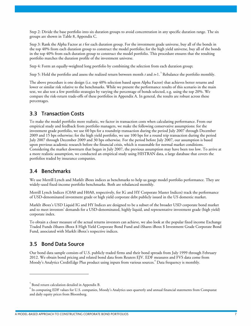
The remainder of this paper is organized as follows: Section 2 briefly reviews the quantitative models supporting our model-based approach. Section 3 describes the model-based investment strategy. Section 4 presents the performance results of the investment strategy. Section 5 provides a summary and conclusion.

2 The Quantitative Models for Risk Measurement and Valuation The quantitative tools supporting our model-based approach are Moody’s Analytics’ EDF (Expected Default Frequency) credit measures and Fair-value Spread (FVS) valuation framework. The EDF credit measure is calculated using a structural framework conceptually similar to the Black-Scholes-Merton (BSM) framework. The intuition behind the EDF model is that the equity of a firm is like a call option on the firm’s underlying assets. The value of the equity thus depends upon, among other things, the market value of the firm’s assets, their volatility, and the payment terms of the liabilities. Implicit in the value of the option is a measure of the probability of the option being exercised; for equity it is the probability of not defaulting on the firm’s liabilities. This structural framework has been further developed over the years by Vasicek and Kealfoher (2003) and others at Moody’s Analytics, with more sophisticated specification and robust empirical implementation than the original BSM model, to become the Public Firm EDF Model.

Like many structured models, the Public Firm EDF Model measures default risk by capturing a company’s financial risk and business risk. The financial risk is the market leverage, which represents how much equity cushion the borrower’s business has as a protection of creditor’s interest; it also measures the distance between the current asset value and the liabilities or the default barrier. The business risk is the asset volatility, which represents the likelihood of a certain percentage shock to the asset value, a shock that may bring the asset value closer to the default barrier. The model uses these two risk factors to help calculate the distance-to-default (DD), which measures how many standard deviations the current asset value is above the default barrier. Using empirical default experience from the past several decades, the DD measure is further mapped to a default probability measure, the resulting Expected Default Frequency (EDF) measure. Over the past twenty years and through multiple economic cycles, the EDF measure has shown superior ability in differentiating, ex ante, defaulting companies from surviving ones; it is also widely used by credit analysts, risk managers, and portfolio managers. For further details regarding the Public Firm EDF Model, please see Dwyer and Qu (2007).

Built upon the EDF model framework, Moody’s Analytics has further developed a valuation framework for modeling credit spreads. The resulting Fair-value Spread (FVS) can be used for valuing credit instruments, such as corporate bonds, loans, and credit derivatives. With the EDF metric as the measure of default risk, the FVS framework incorporates recovery risk, market risk premium, term, and other drivers to derive a modeled spread for the instrument being valued.2 This modeled spread can be compared with the observed spread and the gap used as a relative value indicator during the investment process. This idea is the basis of our investment strategy, which we discuss next.

2 See Appendix A for FVS framework details.

6

3 Investment Strategy The basic intuition behind our investment strategy is straightforward: we buy bonds with the “cheapest” spreads relative to their credit risk. In order to achieve this basic setup, we utilize our measures of default risk and relative value. For default risk, we employ EDF credit measures. For relative value, we use Fair-value Spreads. We also implement an algorithm to control for duration risk and limit the total number of bonds in the portfolio to a reasonable scale.

3.1 Determining the Number of Bonds in Model Portfolios Diversification in credit portfolios is important, because a few concentrated defaults or spread blowups can be extremely detrimental to a portfolio’s performance. A well-diversified portfolio with a large number of bonds can mitigate concentration risk. On the other hand, the cost of creating such a portfolio can be prohibitive to many investors. A passive portfolio usually mimics the existing index, which typically consists of a large number of debt securities. For example, the Merrill Lynch Indices reference thousands of bonds. To reconcile these two conflicting goals, we need to construct a reasonably well-diversified diversified portfolio using a realistic number of bonds.

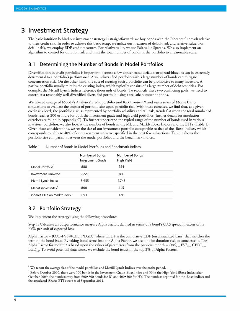
We take advantage of Moody’s Analytics’ credit portfolio tool RiskFrontier™ and run a series of Monte Carlo simulations to evaluate the impact of portfolio size upon portfolio risk. With these exercises, we find that, at a given credit risk level, the portfolio risk, as represented by portfolio volatility and tail risk, trends flat when the total number of bonds reaches 200 or more for both the investment grade and high yield portfolios (further details on simulation exercises are found in Appendix C). To further understand the typical range of the number of bonds used in various investors’ portfolios, we also look at the number of bonds in the ML and MarkIt iBoxx Indices and the ETFs (Table 1). Given these considerations, we set the size of our investment portfolio comparable to that of the iBoxx Indices, which corresponds roughly to 40% of our investment universe, specified in the next few subsections. Table 1 shows the portfolio size comparison between the model portfolios and the benchmark indices.

Table 1 Number of Bonds in Model Portfolios and Benchmark Indices

Number of Bonds Investment Grade

Number of Bonds High Yield

Model Portfolio3 888 314

Investment Universe 2,221 786

Merrill Lynch Index 3,655 1,743

Markit iBoxx Index4 800 445

iShares ETFs on MarkIt iBoxx 693 476

3.2 Portfolio Strategy We implement the strategy using the following procedure:

Step 1: Calculate an outperformance measure Alpha Factor, defined in terms of a bond’s OAS spread in excess of its FVS, per unit of expected loss:

Alpha Factor = (OAS-FVS)/(CEDF*LGD), where CEDF is the cumulative EDF (on annualized basis) that matches the term of the bond issue. By taking bond terms into the Alpha Factor, we account for duration risk to some extent. The Alpha Factor for month t is based upon the values of parameters from the previous month – OASit-1, FVSit-1, CEDFit-1, LGDit-1. To avoid potential data issues, we exclude the bond issues in the top 2% of Alpha Factors.

3 We report the average size of the model portfolios and Merrill Lynch Indices over the entire period.

4 Before October 2009, there were 100 bonds in the Investment Grade iBoxx Index and 50 in the High Yield iBoxx Index; after

October 2009, the numbers vary from 600•800 bonds for IG and 400•500 for HY. The numbers reported for the iBoxx indices and the associated iShares ETFs were as of September 2011.


Step 2: Divide the base portfolio into six duration groups to avoid concentration in any specific duration range. The six groups are shown in Table 8, Appendix C.

Step 3: Rank the Alpha Factor at t for each duration group. For the investment grade universe, buy all of the bonds in the top 40% from each duration group to construct the model portfolio; for the high yield universe, buy all of the bonds in the top 40% from each duration group to construct the model portfolio. This procedure ensures that the resulting portfolio matches the duration profile of the investment universe.

Step 4: Form an equally-weighted long portfolio by combining the selection from each duration group;

Step 5: Hold the portfolio and assess the realized return between month t and t+1. 5 Rebalance the portfolio monthly.

The above procedure is one design (i.e. top 40% selection based upon Alpha Factor) that achieves better returns and lower or similar risk relative to the benchmarks. While we present the performance results of this scenario in the main text, we also test a few portfolio strategies by varying the percentage of bonds selected, e.g. using the top 20%. We compare the risk-return trade-offs of these portfolios in Appendix A. In general, the results are robust across these percentages.

3.3 Transaction Costs To make the model portfolio more realistic, we factor in transaction costs when calculating performance. From our empirical study and feedback from portfolio managers, we make the following conservative assumptions: for the investment grade portfolio, we use 60 bps for a roundtrip transaction during the period July 2007 through December 2009 and 15 bps otherwise; for the high yield portfolio, we use 100 bps for a round trip transaction during the period July 2007 through December 2009 and 30 bps otherwise. For the period before July 2007, our assumption is based upon previous academic research before the financial crisis, which is reasonable for normal market conditions. Considering the market downturn that began in July 2007, the previous assumption may have been too low. To arrive at a more realistic assumption, we conducted an empirical study using HISTRAN data, a large database that covers the portfolios traded by insurance companies.

3.4 Benchmarks We use Merrill Lynch and MarkIt iBoxx indices as benchmarks to help us gauge model portfolio performance. They are widely-used fixed-income portfolio benchmarks. Both are rebalanced monthly.

Merrill Lynch Indices (C0A0 and H0A0, respectively, for IG and HY Corporate Master Indices) track the performance of USD-denominated investment grade or high yield corporate debt publicly issued in the US domestic market.

MarkIt iBoxx’s USD Liquid IG and HY Indices are designed to be a subset of the broader USD corporate bond market and to meet investors’ demands for a USD-denominated, highly liquid, and representative investment grade (high yield) corporate index.

To obtain a closer measure of the actual returns investors can achieve, we also look at the popular fixed income Exchange Traded Funds iShares iBoxx $ High Yield Corporate Bond Fund and iShares iBoxx $ Investment Grade Corporate Bond Fund, associated with MarkIt iBoxx’s respective indices.

3.5 Bond Data Source Our bond data sample consists of U.S. publicly traded firms and their bond spreads from July 1999 through February 2012. We obtain bond pricing and related bond data from Reuters EJV. EDF measures and FVS data come from Moody’s Analytics CreditEdge Plus product using inputs from various sources.6 Data frequency is monthly.

5 Bond return calculation detailed in Appendix B.

6 In computing EDF values for U.S. companies, Moody’s Analytics uses quarterly and annual financial statements from Compustat

and daily equity prices from Bloomberg.

8

3.6 Bond Selection Rules for Investment Universe We only include bonds that meet the following criteria, in addition to other criterion applied by Merrill Lynch Indices:

» Bond issuer is a U.S. publicly traded company with a Moody’s Analytics EDF credit measure

» Bond pays a fixed coupon and has no special features, i.e., is not convertible, putable, etc.

» At least one year remaining term to maturity

» Debt type is preferably senior unsecured

» Rated by Moody’s or S&P

» Amount outstanding must be equal to or greater than $250 million for Investment Grade and $100 million for High Yield

» The bond has been traded recently, according to CAI (Capital Access International) or TRACE data.

» Bond price greater than $40 at time of selection. This filter is used to control the data quality to prevent highly distressed debt or any data errors from entering into the data sample. When tracking the return the following month, the price may drop below $40, and we still calculate the return using the actual price.

Given the above data selection rules, there may be multiple bonds per issuer, the same as with the benchmark indices. The investment universe is constructed using constituents of the Merrill Lynch Indices. The model portfolios are constructed as a subset of the Merrill Lynch Indices after applying the selection rules and the investment strategy. The back-testing period runs from July 1999 through February 2012, and we track the portfolio returns from August 1999 through February 2012. We use this time period in tracking the returns throughout the rest of the paper, unless otherwise specified. We present performance results in the next section.


4 Model Portfolio Performance This section presents the performance of our investment grade and high yield model portfolios. Both portfolios outperform their respective benchmark indices with less or similar risk.

4.1 Investment Grade Model Portfolio Performance Figure 1 shows the comparison of total cumulative returns between our Investment Grade Model Portfolio and the respective Merrill Lynch Index. During August 1999 through February 2012, the IG model portfolio significantly outperforms the Merrill Lynch Index, with an excess return of 2.29% per annum. We achieve an average annualized return of 9.36%, with lower volatility, 5.74% vs. 5.80%, than the ML Investment Grade Index benchmark.

Figure 1 Outperforming the Merrill Lynch Investment Grade Index with lower volatility.

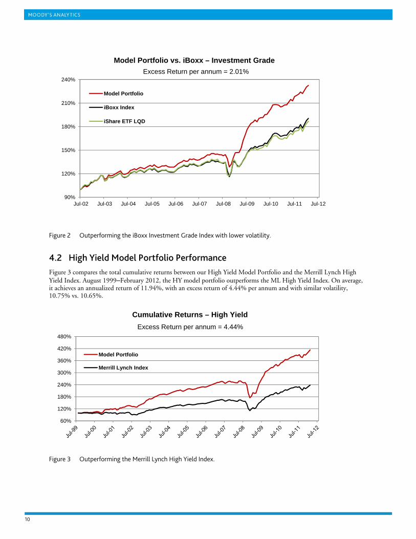
Figure 2 shows the comparison of the total cumulative returns between the IG model portfolio and the iBoxx Investment Grade Index. August 2002 –February 2012, the IG model portfolio significantly outperforms the iBoxx Investment Grade Index, with an excess return of 2.01% per annum and with lower volatility, 5.74% vs. 6.27%, than the MarkIt iBoxx Investment Grade Index.

90%

120%

150%

180%

210%

240%

270%

300%

330%

Cumulative Returns – Investment Grade

Model Portfolio

Merrill Lynch Index

Excess Return per annum = 2.29%

10

Figure 2 Outperforming the iBoxx Investment Grade Index with lower volatility.

4.2 High Yield Model Portfolio Performance Figure 3 compares the total cumulative returns between our High Yield Model Portfolio and the Merrill Lynch High Yield Index. August 1999–February 2012, the HY model portfolio outperforms the ML High Yield Index. On average, it achieves an annualized return of 11.94%, with an excess return of 4.44% per annum and with similar volatility, 10.75% vs. 10.65%.

Figure 3 Outperforming the Merrill Lynch High Yield Index.

90%

120%

150%

180%

210%

240%

Jul-02 Jul-03 Jul-04 Jul-05 Jul-06 Jul-07 Jul-08 Jul-09 Jul-10 Jul-11 Jul-12

Model Portfolio vs. iBoxx – Investment Grade

Model Portfolio

iBoxx Index

iShare ETF LQD


60%

120%

180%

240%

300%

360%

420%

480%

Cumulative Returns – High Yield

Model Portfolio

Merrill Lynch Index



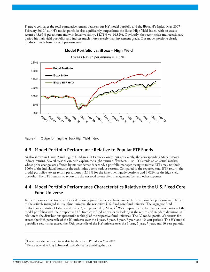
Figure 4 compares the total cumulative returns between our HY model portfolio and the iBoxx HY Index. May 2007–February 2012,7 our HY model portfolio also significantly outperforms the iBoxx High Yield Index, with an excess return of 3.65% per annum and with lower volatility, 14.71% vs. 14.82%. Obviously, the recent crisis and recessionary period hit high yield portfolios and indices much more severely than investment grade. Our model portfolio clearly produces much better overall performance.

Figure 4 Outperforming the iBoxx High Yield Index.

4.3 Model Portfolio Performance Relative to Popular ETF Funds As also shown in Figure 2 and Figure 4, iShares ETFs track closely, but not exactly, the corresponding MarkIt iBoxx indices’ returns. Several reasons can help explain the slight return differences. First, ETFs trade on an actual market, whose price changes are affected by market demand; second, a portfolio manager trying to mimic ETFs may not hold 100% of the individual bonds in the cash index due to various reasons. Compared to the reported total ETF return, the model portfolio’s excess return per annum is 2.14% for the investment grade portfolio and 4.02% for the high yield portfolio. The ETF returns we report are the net total return after management fees and other expenses.

4.4 Model Portfolio Performance Characteristics Relative to the U.S. Fixed Core Fund Universe

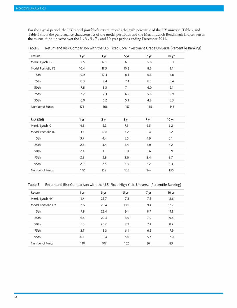
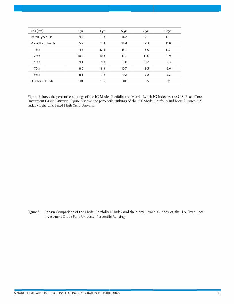
In the previous subsections, we focused on using passive indices as benchmarks. Now we compare performance relative to the actively managed mutual fund universe, the respective U.S. fixed core fund universe. The aggregate fund performance statistics (Table 2 and Table 3) are provided by Mercer.8 We compare the performance characteristics of the model portfolios with their respective U.S. fixed core fund universes by looking at the return and standard deviation in relation to the distributions (percentile ranking) of the respective fund universes. The IG model portfolio’s returns far exceed the 95th percentile of the IG universe over the 1-year, 3-year, 5-year, 7-year, and 10-year periods. The HY model portfolio’s returns far exceed the 95th percentile of the HY universe over the 3-year, 5-year, 7-year, and 10-year periods.

7 The earliest date we can retrieve data for the iBoxx HY Index is May 2007.

8 We are grateful to Amy Labanowski and Mercer for providing the data.

60%

80%

100%

120%

140%

160%

180%

Model Portfolio vs. iBoxx – High Yield

Model Portfolio

iBoxx Index

iShare ETF HYG


12

For the 1-year period, the HY model portfolio’s return exceeds the 75th percentile of the HY universe. Table 2 and Table 3 show the performance characteristics of the model portfolios and the Merrill Lynch Benchmark Indices versus the mutual fund universe over the 1-, 3-, 5-, 7-, and 10-year periods ending December 2011.

Table 2 Return and Risk Comparison with the U.S. Fixed Core Investment Grade Universe (Percentile Ranking)

Return 1 yr 3 yr 5 yr 7 yr 10 yr

Merrill Lynch IG 7.5 12.1 6.6 5.6 6.3

Model Portfolio IG 10.4 17.3 10.8 8.6 9.1

5th 9.9 12.4 8.1 6.8 6.8

25th 8.3 9.4 7.4 6.3 6.4

50th 7.8 8.3 7 6.0 6.1

75th 7.2 7.3 6.5 5.6 5.9

95th 6.0 6.2 5.1 4.8 5.3

Number of Funds 175 166 157 155 145

Risk (Std) 1 yr 3 yr 5 yr 7 yr 10 yr

Merrill Lynch IG 4.3 5.2 7.3 6.5 6.2

Model Portfolio IG 3.7 6.0 7.2 6.4 6.2

5th 3.7 4.4 5.5 4.9 5.1

25th 2.6 3.4 4.4 4.0 4.2

50th 2.4 3 3.9 3.6 3.9

75th 2.3 2.8 3.6 3.4 3.7

95th 2.0 2.5 3.3 3.2 3.4

Number of Funds 172 159 152 147 136

Table 3 Return and Risk Comparison with the U.S. Fixed High Yield Universe (Percentile Ranking)

Return 1 yr 3 yr 5 yr 7 yr 10 yr

Merrill Lynch HY 4.4 23.7 7.3 7.3 8.6

Model Portfolio HY 7.6 29.4 10.1 9.4 12.2

5th 7.8 25.4 9.1 8.7 11.2

25th 6.4 22.3 8.0 7.9 9.4

50th 5.3 20.7 7.3 7.4 8.7

75th 3.7 18.3 6.4 6.5 7.9

95th -0.1 16.4 5.0 5.7 7.0

Number of Funds 110 107 102 97 83

A MOD

DEL-BASED APPRO

Risk (Std)

Merrill Lyn

Model Por

5th

25th

50th

75th

95th

Number of

Figure 5 shInvestmentIndex vs. th

Figure 5

OACH TO CONSTR

nch HY

tfolio HY

f Funds

hows the percent Grade Univershe U.S. Fixed H

Return CompaInvestment Gr

RUCTING CORPO

1 yr

9.6

5.9

11.6

10.0

9.1

8.0

6.1

110

ntile rankings ofse. Figure 6 sho

High Yield Univ

arison of the Mrade Fund Univ

RATE BOND PORT

3 yr

11.3

11.4

12.5

10.3

9.3

8.3

7.2

106

f the IG Modelows the percentverse.

Model Portfolio verse (Percentil

TFOLIOS

5 yr

14.2

14.4

15.1

12.7

11.8

10.7

9.2

101

l Portfolio and Mtile rankings of

IG Index and tle Ranking)

7 yr

12.1

12.3

13.0

11.0

10.2

9.5

7.8

95

Merrill Lynch Ithe HY Model

he Merrill Lync

10 yr

11.1

11.0

11.7

9.9

9.3

8.6

7.2

81

IG Index vs. thl Portfolio and M

ch IG Index vs. t

he U.S. Fixed CMerrill Lynch H

the U.S. Fixed C

1

Core HY

Core

3

14

Figure 6

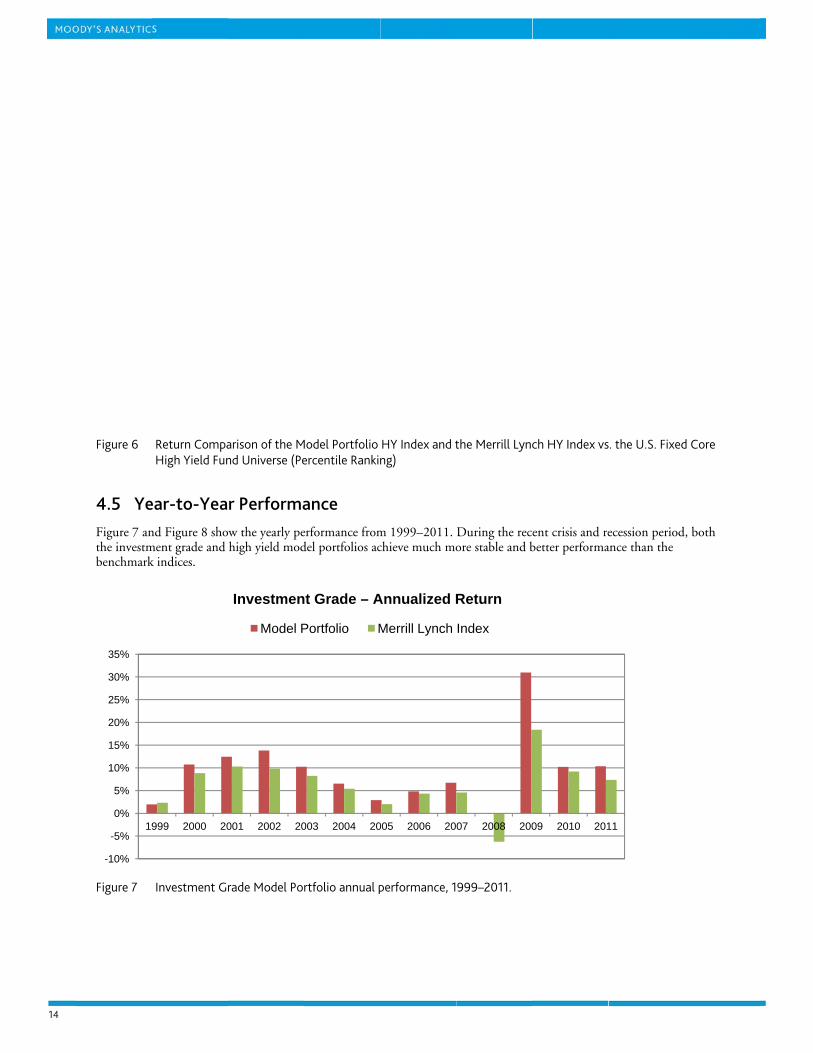
4.5 YeFigure 7 anthe investmbenchmark

Figure 7

-10%

-5%

0%

5%

10%

15%

20%

25%

30%

35%

19

Return CompaHigh Yield Fun

ear-to-Yeand Figure 8 shoment grade and k indices.

Investment Gr

999 2000 20

arison of the Mnd Universe (Pe

r Performaw the yearly pehigh yield mod

rade Model Po

001 2002 20

Investmen

Model P

Model Portfolio ercentile Rankin

ance erformance fromdel portfolios ac

rtfolio annual p

003 2004 20

nt Grade – A

Portfolio M

HY Index and tng)

m 1999–2011. chieve much mo

performance, 1

005 2006 20

Annualized R

Merrill Lynch

the Merrill Lync

During the recore stable and b

999–2011.

07 2008 200

Return

Index

ch HY Index vs

ent crisis and rebetter performa

09 2010 201

s. the U.S. Fixed

ecession periodance than the

11

d Core

d, both


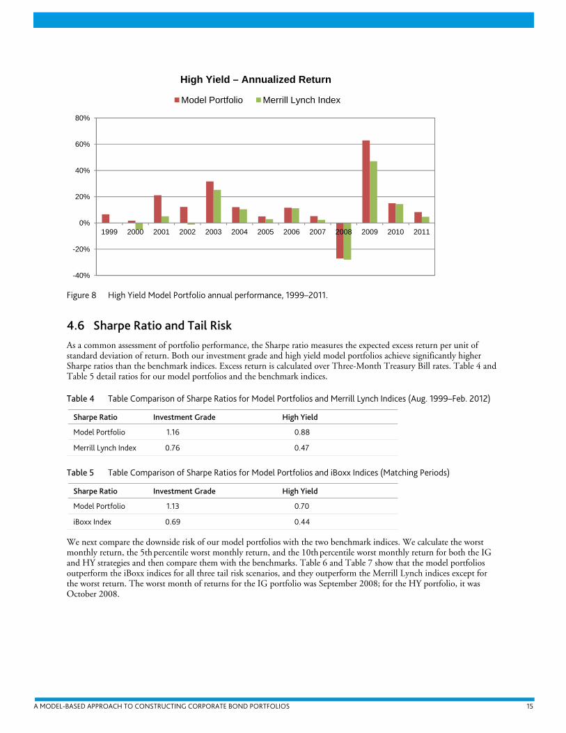
Figure 8 High Yield Model Portfolio annual performance, 1999–2011.

4.6 Sharpe Ratio and Tail Risk As a common assessment of portfolio performance, the Sharpe ratio measures the expected excess return per unit of standard deviation of return. Both our investment grade and high yield model portfolios achieve significantly higher Sharpe ratios than the benchmark indices. Excess return is calculated over Three-Month Treasury Bill rates. Table 4 and Table 5 detail ratios for our model portfolios and the benchmark indices.

Table 4 Table Comparison of Sharpe Ratios for Model Portfolios and Merrill Lynch Indices (Aug. 1999–Feb. 2012)

Sharpe Ratio Investment Grade High Yield

Model Portfolio 1.16 0.88

Merrill Lynch Index 0.76 0.47

Table 5 Table Comparison of Sharpe Ratios for Model Portfolios and iBoxx Indices (Matching Periods)

Sharpe Ratio Investment Grade High Yield

Model Portfolio 1.13 0.70

iBoxx Index 0.69 0.44

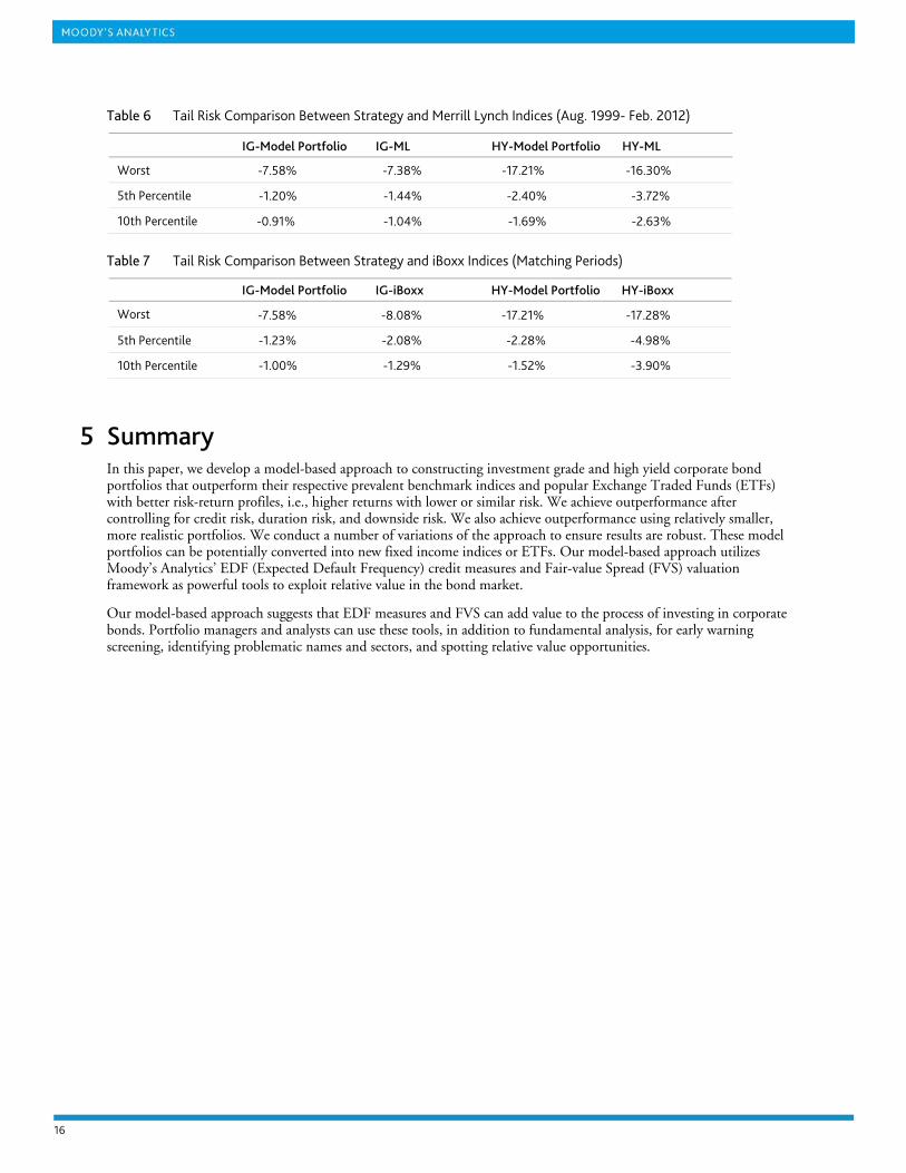
We next compare the downside risk of our model portfolios with the two benchmark indices. We calculate the worst monthly return, the 5th percentile worst monthly return, and the 10th percentile worst monthly return for both the IG and HY strategies and then compare them with the benchmarks. Table 6 and Table 7 show that the model portfolios outperform the iBoxx indices for all three tail risk scenarios, and they outperform the Merrill Lynch indices except for the worst return. The worst month of returns for the IG portfolio was September 2008; for the HY portfolio, it was October 2008.

-40%

-20%

0%

20%

40%

60%

80%

1999 2000 2001 2002 2003 2004 2005 2006 2007 2008 2009 2010 2011

High Yield – Annualized Return

Model Portfolio Merrill Lynch Index

16

Table 6 Tail Risk Comparison Between Strategy and Merrill Lynch Indices (Aug. 1999- Feb. 2012)

IG-Model Portfolio IG-ML HY-Model Portfolio HY-ML

Worst -7.58% -7.38% -17.21% -16.30%

5th Percentile -1.20% -1.44% -2.40% -3.72%

10th Percentile -0.91% -1.04% -1.69% -2.63%

Table 7 Tail Risk Comparison Between Strategy and iBoxx Indices (Matching Periods)

IG-Model Portfolio IG-iBoxx HY-Model Portfolio HY-iBoxx

Worst -7.58% -8.08% -17.21% -17.28%

5th Percentile -1.23% -2.08% -2.28% -4.98%

10th Percentile -1.00% -1.29% -1.52% -3.90%

5 Summary In this paper, we develop a model-based approach to constructing investment grade and high yield corporate bond portfolios that outperform their respective prevalent benchmark indices and popular Exchange Traded Funds (ETFs) with better risk-return profiles, i.e., higher returns with lower or similar risk. We achieve outperformance after controlling for credit risk, duration risk, and downside risk. We also achieve outperformance using relatively smaller, more realistic portfolios. We conduct a number of variations of the approach to ensure results are robust. These model portfolios can be potentially converted into new fixed income indices or ETFs. Our model-based approach utilizes Moody’s Analytics’ EDF (Expected Default Frequency) credit measures and Fair-value Spread (FVS) valuation framework as powerful tools to exploit relative value in the bond market.

Our model-based approach suggests that EDF measures and FVS can add value to the process of investing in corporate bonds. Portfolio managers and analysts can use these tools, in addition to fundamental analysis, for early warning screening, identifying problematic names and sectors, and spotting relative value opportunities.


Appendix A Fair-value Spread Framework On a conceptual level, credit spreads reflect investors’ required compensation for taking on credit risk, which predominantly includes both default and recovery risk. Higher default and loss given default translate into higher spreads. Credit spreads also reflect investors’ attitudes toward risk over time. If investors are more risk averse, say in 2009 than in 2008, they require more spreads for the same amount of default and recovery risk. Furthermore, borrower systematic risk and its correlation within the general economy also have an impact upon credit spreads. Higher systematic risk implies that it is more difficult to diversify away risk; hence, investors require higher spreads to include the bond in their portfolios. Therefore, a model for credit spreads should incorporate at least these inputs: default probabilities, loss given default, risk premium, and systematic risk.

To make the above argument more rigorous, we follow the risk-neutral valuation methodology grounded in the No-Arbitrage principle. More specifically, we compute a transformation that converts our default probabilities under the physical measure (EDF credit measures) to default probabilities under the risk-neutral measure (Quasi Default Frequencies or QDFs). The main parameter in this transformation is the market price of risk (denoted by λ here). This parameter captures corporate debt investors’ attitudes toward risk. Alternatively, λ can be interpreted as the market Sharpe ratio or the expected excess return demanded by investors per unit of risk. This attitude toward risk for credit market investors is best reflected in the prices (or spreads) of credit risky claims. Consequently, we use these data to calibrate the market Sharpe ratio.

Under the risk-neutral valuation principle, the model spread, or Fair-value Spread, on a defaultable zero-coupon bond, is given by:

1 ln(1 * )

1 *

T T

T

FVS CQDF LGDT

CQDF LGDT

= − −

≈

(1)

Where T is the tenor of the bond, CQDF is the cumulative default probability under the risk-neutral measure, and LGD is the loss given default. Although the above equation is derived for zero-coupon bonds, the relationship works reasonably well for coupon-bearing bonds, with T replaced by its duration.

The above equation suggests that spreads should be approximately equal to expected loss under the risk-neutral measure. To calculate the CQDFs, we begin with EDF credit measures, our default probabilities under the physical measure. When asset returns are assumed to follow a Geometric Brownian motion process, one can show that CQDF can be obtained from CEDF through the following transformation,9

( )1 iiT iT

i

rCQDF N N CEDF Tμσ

−⎡ ⎤−= +⎢ ⎥

⎣ ⎦ (2)

9 See Agrawal, et al, (2004) for a derivation.

18

In our valuation framework, we rewrite this relationship by imposing the Capital Asset Pricing Model (CAPM) on asset returns. CAPM says,

( ) ( )

( )

( ) ( )

( )

2

1

i im m

im i mm

m

i mim

i m

i im m

iT iT im m

r r

r

r r

CQDF N N CEDF T

μ β μρ σ σ μσ

μ μρ

σ σλ ρ λ

ρ λ−

− = −

= −

− −=

=

⇒

⎡ ⎤= +⎣ ⎦

(3)

Thus,

( )11 ln(1 )T iT im mFVS N N CEDF T LGDT

ρ λ−⎡ ⎤= − − + ×⎣ ⎦ (4)

Because CEDF is known and LGD values can be estimated separately, ρim and λm are the two main unknown parameters. ρim is the correlation coefficient of individual asset returns with the market returns and represents a firm-specific parameter. The market Sharpe ratio is constant across the entire cross-section of assets. Conceptually, both parameters can vary over time.

While the model in Equation (4) works, in general, one systematic bias that appears in the bond spreads is the “size effect.” We find that the spreads on bonds issued by smaller firms are systematically higher than those on bonds of larger firms, even after controlling for various known spread drivers such as EDF credit measure, agency rating, seniority, tenor, and industry. We take such findings as clear evidence of a size effect in bond spreads, which is not too surprising given the long history of a known size effect in the stock market. We capture the size effect by (a) calibrating the model in Equation (4) to large firms only and (b) including a Size Premium term to explain the spreads for small firms.

Thus, the general model with Size Premium becomes

( ) ( )11 ln(1 )T z i iT im mS f z N N CEDF T LGDT

β ρ λ−⎡ ⎤= − − + ×⎣ ⎦ (5)

where z is the firm size, f(z) is a size-function whose form is calibrated from the bond data, βz is the Size Premium

parameter, and β z f(zi) is the Size Premium.


Appendix B Calculation of Bond Return We calculate total returns, including price changes and coupon income, and include accrued interest. For simplicity, we exclude income from reinvestment.10 We calculate the bond return for month t as follows:

1t1t

1ttt AIP

PδCPR

−−

−

+−×+

= (6)

Where Pt-1 is the price of the bond at the end of month t-1;

AIt-1 is the accrued interest at the end of month t-1;

Pt is the price of the bond at the end of month t;

C is the coupon payment;

δ is the number of days in month t /365.25

Coupon payments are assumed at month’s end.

The return of a bond portfolio for month t is calculated as follows:

∑=

×=tN

1iitit

pt Rw R

(7)

Where Nt is the number of bonds in the sample in month t;

Rit is the return on bond i for month t.

Return on the existing index is value-weighted as standard. Our model portfolio is equally-weighted constructed. Wit = 1/Nt

10

Including the reinvestment income would increase strategy returns and does not change the conclusion of our results.

20

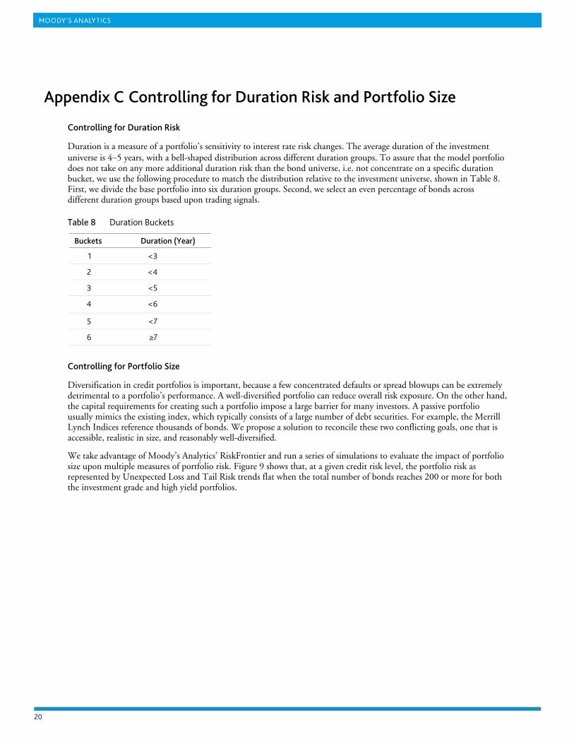
Appendix C Controlling for Duration Risk and Portfolio Size

Controlling for Duration Risk

Duration is a measure of a portfolio’s sensitivity to interest rate risk changes. The average duration of the investment universe is 4–5 years, with a bell-shaped distribution across different duration groups. To assure that the model portfolio does not take on any more additional duration risk than the bond universe, i.e. not concentrate on a specific duration bucket, we use the following procedure to match the distribution relative to the investment universe, shown in Table 8. First, we divide the base portfolio into six duration groups. Second, we select an even percentage of bonds across different duration groups based upon trading signals.

Table 8 Duration Buckets

Buckets Duration (Year)

1 <3

2 <4

3 <5

4 <6

5 <7

6 ≥7

Controlling for Portfolio Size

Diversification in credit portfolios is important, because a few concentrated defaults or spread blowups can be extremely detrimental to a portfolio’s performance. A well-diversified portfolio can reduce overall risk exposure. On the other hand, the capital requirements for creating such a portfolio impose a large barrier for many investors. A passive portfolio usually mimics the existing index, which typically consists of a large number of debt securities. For example, the Merrill Lynch Indices reference thousands of bonds. We propose a solution to reconcile these two conflicting goals, one that is accessible, realistic in size, and reasonably well-diversified.

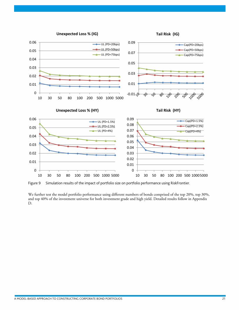
We take advantage of Moody’s Analytics’ RiskFrontier and run a series of simulations to evaluate the impact of portfolio size upon multiple measures of portfolio risk. Figure 9 shows that, at a given credit risk level, the portfolio risk as represented by Unexpected Loss and Tail Risk trends flat when the total number of bonds reaches 200 or more for both the investment grade and high yield portfolios.


Figure 9 Simulation results of the impact of portfolio size on portfolio performance using RiskFrontier.

We further test the model portfolio performance using different numbers of bonds comprised of the top 20%, top 30%, and top 40% of the investment universe for both investment grade and high yield. Detailed results follow in Appendix D.

0

0.01

0.02

0.03

0.04

0.05

0.06

10 30 50 80 100 200 500 1000 5000

Unexpected Loss % (IG)

UL (PD=20bps)

UL (PD=50bps)

UL (PD=75bps)

‐0.01

0.01

0.03

0.05

0.07

0.09

Tail Risk (IG)

Cap(PD=20bps)

Cap(PD=50bps)

Cap(PD=75bps)

0

0.01

0.02

0.03

0.04

0.05

0.06

10 30 50 80 100 200 500 1000 5000

Unexpected Loss % (HY)

UL (PD=1.5%)

UL (PD=2.5%)

UL (PD=4%)

0

0.01

0.02

0.03

0.04

0.05

0.06

0.07

0.08

0.09

10 30 50 80 100 200 500 10005000

Tail Risk (HY)

Cap(PD=1.5%)

Cap(PD=2.5%)

Cap(PD=4%)

22

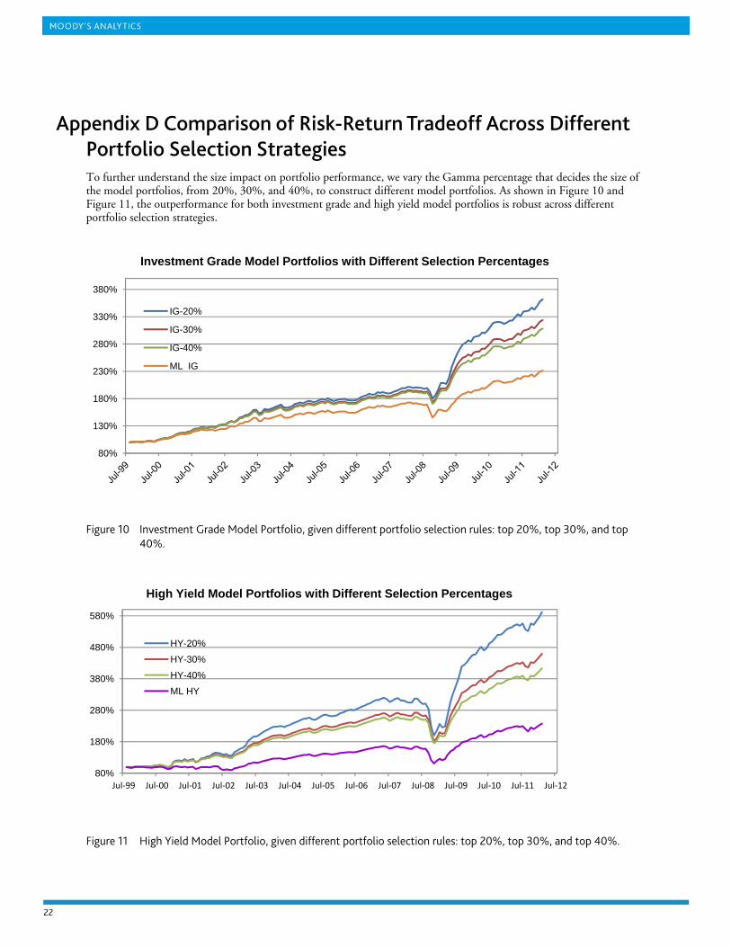
Appendix D Comparison of Risk-Return Tradeoff Across Different Portfolio Selection Strategies To further understand the size impact on portfolio performance, we vary the Gamma percentage that decides the size of the model portfolios, from 20%, 30%, and 40%, to construct different model portfolios. As shown in Figure 10 and Figure 11, the outperformance for both investment grade and high yield model portfolios is robust across different portfolio selection strategies.

Figure 10 Investment Grade Model Portfolio, given different portfolio selection rules: top 20%, top 30%, and top

40%.

Figure 11 High Yield Model Portfolio, given different portfolio selection rules: top 20%, top 30%, and top 40%.

80%

130%

180%

230%

280%

330%

380%

IG-20%

IG-30%

IG-40%

ML IG

Investment Grade Model Portfolios with Different Selection Percentages

80%

180%

280%

380%

480%

580%

Jul‐99 Jul‐00 Jul‐01 Jul‐02 Jul‐03 Jul‐04 Jul‐05 Jul‐06 Jul‐07 Jul‐08 Jul‐09 Jul‐10 Jul‐11 Jul‐12

HY-20%

HY-30%

HY-40%

ML HY

High Yield Model Portfolios with Different Selection Percentages


Table 9 shows the risk-return comparison for the different selection percentage model portfolios. Both the return and the risk decrease with an increase in portfolio size.

Table 9 Risk-Return Comparison for Different Selection Percentage Model Portfolios

Portfolio Return Volatility

Strategy. IG (TOP 20%) 10.76% 6.24%

Strategy. HY (TOP 20%) 15.18% 13.77%

Strategy. IG (TOP 30%) 9.79% 5.83%

Strategy. HY (TOP 30%) 12.88% 11.49%

Strategy. IG (TOP 40%) 9.36% 5.74%

Strategy. HY (TOP 40%) 11.94% 10.75%

Benchmark (ML IG) 6.89% 5.80%

Benchmark (ML HY) 7.12% 10.65%


References

Acknowledgements

Our thanks to David Munves for his valuable insights throughout the development of the strategy and paper. We would also like to thank Sunny Wong, Chenxue Li, and Yu Zhou for their help with the data.

Copyright © 2012 Moody's Analytics, Inc. and/or its licensors and affiliates. All rights reserved.

References

Black, Fischer, and Myron Scholes, “The Pricing of Options and Corporate Liabilities.” Journal of Political Economy, Vol. 81, No 3, 637–659, 1973.

Agrawal, Deepak, Navneet Arora, and Jeffery R. Bohn, “Parsimony in Practice: An EDF-Based Model of Credit Spreads.” Moody’s KMV, 2004.

Dwyer, Douglas and Irina Korablev, “Power and Level Validation of Moody’s KMV EDF™ Credit Measures in North America, Europe, and Asia.” Moody’s KMV, 2007.

Dwyer, Douglas and Shisheng Qu, “EDF™ 8.0 Model Enhancements.” Moody’s KMV, 2007.

Kealhofer, Stephen, “Quantifying Credit Risk I: Default Prediction.” Financial Analysts Journal, January/February 2003, 30–44, 2003a.

Li, Zan and Jing Zhang, “Investing in Corporate Credit Using Quantitative Tools.” Moody’s Analytics White Paper, 2010.

Li, Zan, Shisheng Qu, and Jing Zhang, “Long-Short Investing and Information Flow between the Equity and Credit Default Swap Markets.” Forthcoming Moody’s Analytics White Paper, 2012.

Korablev, Irina and Shisheng Qu, “Validating the Public EDF Model Performance During the Recent Credit Crisis.” Moody’s Analytics White Paper, 2009.

Miller, Ross, “Refining Ratings.” Risk, Vol. 11, No 8, 97–99, 1998.

Documents

A Model-Based Approach to Constructing Corporate … · A Model-Based Approach to Constructing ... these are issues where ... which employs a similar setup for portfolio construction