A Mixed-Integer Programming Model for Gas Purchase andTransportation

Luis Contesse lcontess@ing.puc.clEngineering School, Catholic University of Chile, Casilla 306, Santiago 22, Chile

Juan Carlos Ferrer jferrer@sloan.mit.eduEngineering School, Catholic University of Chile, Casilla 306, Santiago 22, Chile

Sergio Maturana∗ smaturan@ing.puc.clEngineering School, Catholic University of Chile, Casilla 306, Santiago 22, Chile

April 14, 2005

Abstract

The natural supply chain involves three main agents: producers, transportation companies, and localdistribution companies (LDCs). We present a MIP model that is the basis for a decision support systemdeveloped for a Chilean LDC. This model takes into account many of the complexities of the purchasingand transportation contracts to help optimize daily purchase and transportation decisions in the absenceof local storage facilities. The model was solved to optimality within a reasonable time. We show howthe model handles several contractual issues and give some insights for the case when demand scenariosare used to deal with uncertainty.Keywords: Mixed-Integer Programming, Natural Gas, Logistics.

1 Introduction and Literature ReviewNatural gas is an important source of energy for many users. In many places it is the preferred alternativefor residential heating and cooking. It can also be used by certain industries as an alternative to fuel oil.Although it has been used extensively in the United States for many years, its use in Chile began only in1997, when a 465-kilometer pipeline between southern Argentina and the central part of Chile was completed.The natural gas industry involves three main agents: producers, which are mainly concerned with the

exploration, development and exploitation of gas reserves; gas pipeline companies, which aggregate gas inproduction areas and transport it to consumption areas; and Local Distribution Companies (LDCs), whichprovide gas service to end customers in a particular geographic region. These LDCs have traditionallypurchased their gas supplies from the gas pipeline companies under long-term contracts (twenty or moreyears).LDCs provide natural gas service to residential, commercial, and industrial customers within its service

territory. They have to decide from which producers to purchase the gas and how to transport the gas fromthe wellhead to the end customers, using extensive systems of pipelines and storage facilities. Other formsof transportation (truck, train, or ship) are usually not economically feasible. Storage facilities help absorbdemand fluctuations that may occur during the year. Large commercial and industrial customers can beserved on either a firm or an interruptible basis. Interruptible sales customers are willing to have their gassupply curtailed during periods of peak demands in exchange for a lower price. This type of customer canbe an alternative to the use of storage facilities for absorbing demand fluctuations.

∗The authors are grateful for the research support provided by Conicyt (grant number FONDEF 2-55) and for the valuablehelp received from Eliseo Lopez, from Metrogas and Cristian Villena, Allan Gubbins, Alejandro Ortiz, and the rest of theGESCOPP team in developing this model. We also thank the two anonymous referees for their valuable suggestions and theeditors for their effort in handling the process.

1

Changes in the regulatory system of the gas industry in the United States, which began in 1985, havepresented new supply alternatives to gas purchasers, including Gas Pipeline Companies (GPCs), LDCs, andlarge end users. These changes have encouraged pipeline companies to unbundle their traditional merchantservices and allow buyers to transport their own gas through the pipeline system. This open access to gastransportation services gives gas purchasers the opportunity to buy gas directly from non-pipeline sources,including natural gas producers and independent marketing companies. This is generating an active spotmarket for natural gas.The purchase and transportation of natural gas is governed by very complex contracts. LDCs have to

operate on a daily basis taking into account the conditions stipulated in the contracts and the uncertaintiesof the demand. The residential segment of the market, which is usually the most important one, is difficult topredict on a daily basis since it depends on weather conditions. Low temperatures in the winter can inducea significant increase in natural gas demand. It is very difficult to obtain reliable predictions of weatherconditions with the anticipation required by the planners.One type of contract that has become more common due to the changes in the regulation is the firm

transportation contract, which allows shippers to reserve a portion of the pipeline’s total delivery capacityfor their own use. The shipper pays a monthly demand charge based on the maximum daily delivery quantitycontracted and a transportation charge for each unit delivered. Additional pipeline transportation servicesare available on an interruptible basis, where the shipper pays only for the gas transported.The objective of gas supply planning is to minimize the LDC’s costs. Over the short term, this means

optimally dispatching the available gas supply to meet variable demand. Over the long term, this meansconstructing an optimal portfolio of gas sources including gas purchases from pipelines, storage, and trans-portation of gas purchased directly from producers. Planners need to have a Decision Support System (DSS)to help them determine the best way to satisfy the uncertain demand they face subject to the complex setof conditions specified in the contracts they have signed with their providers and GPCs.Optimization models have been applied to many different problems related to the complex process of

purchasing and transporting natural gas. In particular, Murphy et al. (1981), Levary and Dean (1980), andO’Neill et al. (1979) report on the use of Linear Programming (LP) models for long-term supply planningby the natural gas industry and regulators.An optimal gas supply strategy can only be defined after considering a wide range of purchase, trans-

portation, and gas storage options over a multiyear time horizon. As a consequence, these optimal strategiesshould be determined using large scale optimization models. These models have been successfully used toassist gas supply planners in making both strategic and operational gas supply and transportation decisions.Chin and Vollmann (1992) illustrate the use of methodologies based on Material Requirements Planning(MRP) and LP models as decision support tools for the problem of buying natural gas to meet a weather-dependent demand.The problem of optimizing the selection of supply contracts, which is also called the optimal supply mix

problem, has been studied by several authors. Avery et al. (1992) present a DSS based on a highly detailedoptimization model, used by utilities to plan operations, which minimizes cost while satisfying regulatoryagencies. Knowles and Wirick (1998) describe how “The Peoples Gas Light and Coke Company” plans itsgas supply. They used an optimization model that considers multiple weather scenarios in determining asupply portfolio. With the deregulation of the natural gas industry, the company has used the model torestructure supply portfolios, saving more than $50 millions annually. Guldmann and Wang (1999) proposeda large Mixed-Integer Linear Program (MILP or MIP) and a much smaller Non-Linear Programming (NLP)approximation of the MILP, involving simulation and response surface estimation via regression analysis tosolve the problem of the optimal selection of natural gas supply contracts by LDCs. Each potential supplysource is characterized by several price and nonprice parameters. Weather variability is the main stochasticfactor that drives the demand for gas of the various market segments. The model minimizes the total costof gas supply and market curtailment and determines the size of the interruptible market.Other approaches have used optimization models at a more operational level. De Wolf and Smeers (2000)

formulated the problem of distributing gas through a network of pipelines as a cost minimization subject tononlinear flow-pressure relations, material balances, and pressure bounds. The solution method is based onpiecewise linear approximations of the nonlinear flow-pressure relations. A project which aims at developingan integrated DSS for the optimization of natural gas pipeline operations is described in (Sun et al., 2000).This integrated system uses both expert systems and operations research to model the operations of gas

2

Figure 1: Transportation Network

pipelines.In this article we describe the model we developed for Metrogas, a Chilean LDC, which is part of the

Optimization-Based DSS (OBDSS) that was implemented in the context of a 3-year R&D project calledGESCOPP. This project has produced several prototypes in different areas, one of which is described in(Gazmuri & Maturana, 2001). For a complete description we refer the reader to (Gazmuri et al., 1993). Theremainder of this article is organized as follows. In §2 we describe the problem in detail. In §3 we presentthe MIP model we developed. In §4 we give some details of the implementation of this model at Metrogas.In §5 we discuss an extension using stochastic optimization. Finally, we state our conclusions in §6.

2 Problem DescriptionThe natural gas that supplies the central part of Chile comes from two sources in Argentina: Sierra Chataand Total Austral. It is transported to Chile, across the Andes mountains, through a 465 km. pipeline whichwas completed in August 1997.As shown in Figure 1, the pipeline can be divided into three sections, which belong to three different

GPCs: Transportadora de Gas del Norte (TGN), Gas Andes Argentina (GAA), and Gas Andes Chile (GAC).The gas is purchased directly by Metrogas from the producers and then shipped to Chile through these GPCs.The model that will be described in the next section, maximizes the company’s profit over a certain

planning horizon. The profit is computed as the difference between the total income derived from salesto different end customers and the purchase and transportation costs. Two different types of demand areconsidered: firm and interruptible. Firm demand comes mostly from residential customers. Interruptibledemand comes mostly from industrial customers with interruptible service. At the La Mora node there isalso an external agent who may buy gas from Metrogas at a spot price. Interruptible demand helps dealwith demand fluctuations since storage facilities are very limited. Since the prices for interruptible serviceand for gas sold at La Mora are much lower than the prices for residential customers, selling interruptibleservice or at La Mora only becomes an interesting option when residential demand is low for a relatively longperiod of time (more than one month). Interruptible service customers can resort to an alternative sourceof energy but whenever possible switch to gas, because of the lower price specified in their contracts.The producers, Sierra Chata and Total Austral, have long-term gas supply contracts with Metrogas, with

monthly and quarterly conditions, respectively. These contracts, which extend over twenty years, includepricing provisions to encourage buyers to maintain high purchase factors. There is a minimum monthly orquarterly amount of gas that Metrogas must purchase from the producers, regardless of the end customerdemand. This quantity is the so-called take-or-pay (TOP), which is a fixed volume of gas contracted witheach producer. The total purchase cost is the sum of the fixed TOP cost plus the cost of any additional gasbeyond the TOP level, valued at some fixed commodity rate, i.e., a cost proportional to the volume of gasrequested. In addition, there are some purchase penalty costs (fines) when daily minimum and maximum

3

Figure 2: Make up Generation and Recovery

purchase levels are surpassed.Another important condition specified in the contracts between producers and Metrogas is the make-up

recourse. Make-up is the difference between the TOP level and the volume of gas actually received by thebuyer, when it is below this level (see Figure 2). This make-up may be used, or recovered, when the volumeactually received by the buyer exceeds the TOP level, within the twelve periods immediately following theperiod where it originated, i.e., one or three years depending on whether the periods are months or quarters.After that, the buyer loses it.At the pipeline level, the shippers or transportation companies also establish long-term contracts with

Metrogas. Since the three sections of pipeline work under similar operating conditions, the transportationcontracts have the same structure for the three shippers. They all have a maximum daily quantity (MDQ),which can be shipped at some daily basic demand charge (BDC). If the buyer needs to transport in excessof the MDQ, it can request an authorized overrun gas (AOG) at a higher cost. If the AOG is not requestedor granted, the buyer may incur in an unauthorized overrun gas (UOG) at an even higher cost.If on a given day the shipper is unable to transport the customer’s firm scheduled daily delivery (SDD),

the resulting (positive) delivery deficiency (DD) originated in that day may be accumulated by the customerand used in future periods to diminish overrun transportation costs. On the other hand, if on a given daythe customer does not make use of all of its firm SDD, a (negative) DD is generated which must also becompensated for in the future.Transportation contracts establish complex linepack conditions related to the pipeline’s daily transporta-

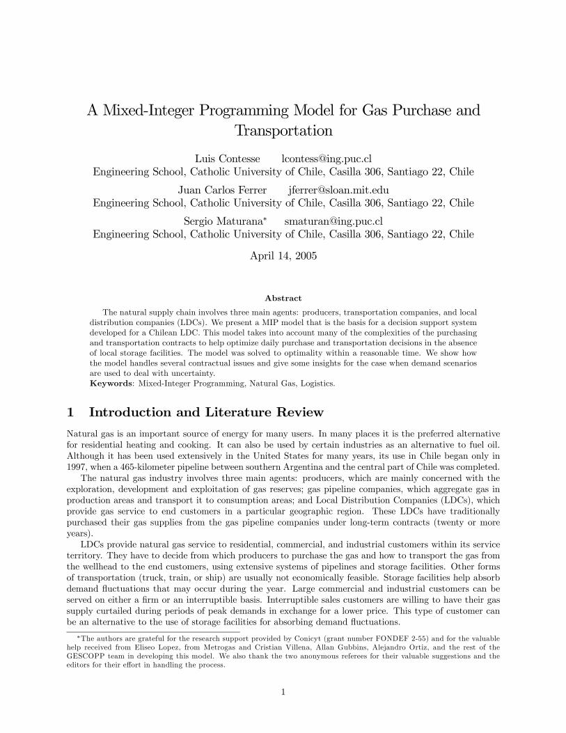
tion capacity. The linepack is the fraction of the pipeline’s total transportation capacity that is owned bythe customer. Any positive or negative linepack unbalances produced by the daily transported quantitieswith to the contracted linepack, are penalized with increasing return to scale costs (see Figure 3).

3 The ModelThere are some assumptions of our model that differ from most models found in the gas literature. Forinstance, the lack of storage facilities in the Chilean pipeline system, which are of great importance in theoperation of US natural gas pipelines, forces us to consider interruptible service and the agent at La Morato handle demand fluctuations. Make-up recovery and linepack unbalances, which are other ways to handlethese fluctuations, can only absorb short-term variations. Interruptible service prices are fixed by long-termcontracts, so they are known in advance. Prices at La Mora, however, are spot prices which were estimatedby experts based on their experience. Another consideration is that we only model the part of the pipelineoperated by Metrogas, not the complete pipeline. That is why we model the loss of gas due to pumping(and other losses) as a fixed proportion of the gas received at each node. It would be necessary to includecompressor considerations if we were modeling the transportation company’s problem.

4

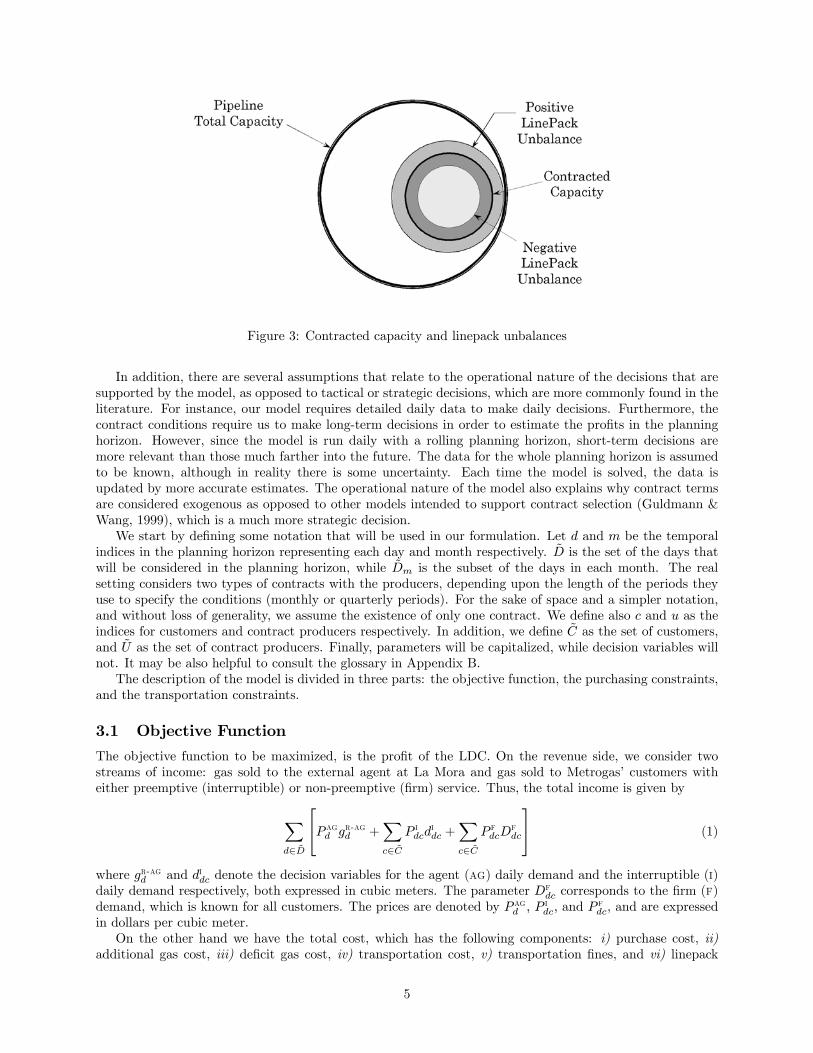
Figure 3: Contracted capacity and linepack unbalances

In addition, there are several assumptions that relate to the operational nature of the decisions that aresupported by the model, as opposed to tactical or strategic decisions, which are more commonly found in theliterature. For instance, our model requires detailed daily data to make daily decisions. Furthermore, thecontract conditions require us to make long-term decisions in order to estimate the profits in the planninghorizon. However, since the model is run daily with a rolling planning horizon, short-term decisions aremore relevant than those much farther into the future. The data for the whole planning horizon is assumedto be known, although in reality there is some uncertainty. Each time the model is solved, the data isupdated by more accurate estimates. The operational nature of the model also explains why contract termsare considered exogenous as opposed to other models intended to support contract selection (Guldmann &Wang, 1999), which is a much more strategic decision.We start by defining some notation that will be used in our formulation. Let d and m be the temporal

indices in the planning horizon representing each day and month respectively. D is the set of the days thatwill be considered in the planning horizon, while Dm is the subset of the days in each month. The realsetting considers two types of contracts with the producers, depending upon the length of the periods theyuse to specify the conditions (monthly or quarterly periods). For the sake of space and a simpler notation,and without loss of generality, we assume the existence of only one contract. We define also c and u as theindices for customers and contract producers respectively. In addition, we define C as the set of customers,and U as the set of contract producers. Finally, parameters will be capitalized, while decision variables willnot. It may be also helpful to consult the glossary in Appendix B.The description of the model is divided in three parts: the objective function, the purchasing constraints,

and the transportation constraints.

3.1 Objective Function

The objective function to be maximized, is the profit of the LDC. On the revenue side, we consider twostreams of income: gas sold to the external agent at La Mora and gas sold to Metrogas’ customers witheither preemptive (interruptible) or non-preemptive (firm) service. Thus, the total income is given by

Xd∈D

P agd gr-agd +Xc∈C

P idcdidc +

Xc∈C

P fdcDfdc

(1)

where gr-agd and didc denote the decision variables for the agent (ag) daily demand and the interruptible (i)daily demand respectively, both expressed in cubic meters. The parameter Df

dc corresponds to the firm (f)demand, which is known for all customers. The prices are denoted by P agd , P

idc, and P

fdc, and are expressed

in dollars per cubic meter.On the other hand we have the total cost, which has the following components: i) purchase cost, ii)

additional gas cost, iii) deficit gas cost, iv) transportation cost, v) transportation fines, and vi) linepack

5

fines. Next, we describe each of these costs.The purchase cost includes all daily nominations for all producers plus all the costs associated with take-

or-pay contracts, which are basically sunk costs and are denoted by Ctop. Thus, the purchase cost is givenby

Cp = Ctop +Xd∈D

Xu∈U

Cgdu · gi2du, (2)

where Cgdu and denote the cost of one cubic meter of gas for both monthly and quarterly contract produc-ers, respectively. The decision variables gi2du represent the volume of injected gas above the monthly TOPthreshold, but within the allowed daily range.When the amount of utilized gas is greater than the maximum daily consumption (cdc) in the contract

(e.g., day 7 in Figure 2), there is a cost for this additional gas given by

Ca =Xd∈D

Xu∈U

Cadu · gadu, (3)

where Cadu are the costs for an additional cubic meter of gas, and gadu are the corresponding decision variables

for the volume of additional gas.Similarly, when the amount of utilized gas is less than the minimum daily consumption specified in the

contract (e.g., day 4 in Figure 2), the cost of the deficit of gas is given by

Cd =Xd∈D

Xu∈U

Cddu · gddu, (4)

where the variables and parameters used are similar to the additional gas cost case.The gas is transported by different transportation companies which belong to the set T , for instance

T = {tgn, gaa, gac}. The companies charge different fees for firm and interruptible quantities. If Cbdcdk isthe Basic Demand Charge (bdc), which is constant in our case although we maintained the daily index forgenerality, and Cpspdk is the daily spot price for a cubic meter of interruptible gas, the transportation cost isgiven by

Ct =Xk∈T

Xd∈D

(Cbdcdk · Gmdqdk + Cpspdk · gidk) (5)

where Gmdqdk is the maximum daily amount of gas transported by company k, and gidk is the decision variableof how much interruptible gas will be transported by the same company.A transportation fine is charged when there is some level of unauthorized overrun gas, uog. These fines

are calculated as a proportion Muogi·dk ∈ [0, 1] of the corresponding bdc. The model considers three different

sections of the pipeline for the transportation fines. Thus the constraint is given by

Ctf =Xk∈T

Xd∈D

Cbdcdk

hP3i=1

¡Muogi0dk · guogi0dk +Muogi

1dk · guogi1dk

¢i. (6)

Lastly, we consider a fine due to linepack unbalances. This fine has four components: the first twoassociated with daily unbalances (positive lp-dp and negative lp-dn) and the other two with cumulativeunbalances (positive lp-cp and negative lp-cn). For linepack fines, this model considers four differentsections in the pipeline. Thus, the fine is given by

Clf =X

i=1,...,4

Xk∈T

Xd∈D

©Cbdcdk ·Mlp-dp

dk · Clp-dpidk · glp-dpidk + Cbdcdk ·Mlp-dndk · Clp-dnidk · glp-dnidk (7)

+Cbdcdk ·Mlp-cpdk · Clp-cpidk · glp-cpidk + Cbdcdk ·M lp-cn

dk · Clp-cnidk · glp-cnidk

ª,

where Mlp-·dk ∈ [0, 1] is the proportion of the corresponding bdc, Clp-·idk is the associated fine of one cubic

meter in section i, and glp-·idk is the decision variable for the amount of linepack gas.Therefore, by adding up (2)-(7) the total cost is given by

C = Cp + Ca + Cd + Ct + Ctf + Clf. (8)

6

3.2 Purchase Constraints

The constraints related to the gas purchase process are the following:

• Injection of gas: There are two types of injection which can be requested to the producers on a givenday: gas injected under the take-or-pay contract, denoted by gi1du ≥ 0, and gas consumed above theTOP threshold, denoted by gi2du ≥ 0, which has a higher cost. The sum of all injections in a singleperiod has to be less than or equal to the TOP Gtopmu for the same period. Thus, for monthly contractproducers we have X

d∈Dm

gi1du · Gtopmu ∀m ·M, ∀u ∈ U . (9)

• Maximum daily consumption: As shown in Figure 2, there is a maximum daily consumption inthe contract (Gcdcdu ) which can be increased by requesting additional gas (g

adu). This quantity has to

be higher than or equal to the sum of injected and recovered gas. The following constraint representsthe previous condition for monthly contract producers:

gi1du + gi2du + g

rdu · G

cdcdu + gadu ∀d ∈ D, ∀u ∈ U .

In addition, it is not always possible to request additional gas. The binary parameter Dadu is equal to

1 when additional gas can be requested in day d from a given producer, 0 otherwise. This restrictionyields the following two constraints:

gadu ≥ 0 if Dadu = 1

gadu = 0 if Dadu = 0.

• Minimum daily consumption: This constraint is similar to the previous one. The total injected gashas to be higher than or equal to the minimum daily consumption in the contract minus the requesteddeficit of gas if possible (Dd

du = 1). These constraints can be expressed as

gi1du + gi2du ≥ Gmindu − g

ddu ∀d ∈ D, ∀u ∈ U (10)

gddu ≥ 0 if Dddu = 1

gddu = 0 if Dddu = 0.

• Make-up generation: If the total gas utilized in a given period is less than the TOP quantity forthe same period, make-up is generated. This is represented by

ggmu = Gtopmu −

Xd∈Dm

gi1du ∀m ·M, ∀u ∈ U . (11)

• Make-up utilization: It is not possible to use make-up in every period. Different producers havedifferent restrictions in that respect. Let Dm

mu be the binary parameters which are equal to 1 for thoseperiods where make-up can be utilized. The associated constraints for monthly contract producers aregiven by X

d∈Dm

grdu = 0 if Dmmu = 0 (12)

Xd∈Dm

grdu ≥ 0 if Dmmu = 1. (13)

• Make-up generation and recovery control: In each period it is possible to generate make-up orto recover gas from make-up, but never both in the same period. In order to enforce this, we introduce

7

the binary decision variables αmu which take a value equal to 1 in those periods when gas recovery isallowed and 0 otherwise. The following constraints reflect this condition:X

d∈Dm

grdu · αmu ·Mbig2 ∀m ·M, ∀u ∈ U , (14)

Xd∈Dm

gi2du · αmu ·Mbig2 ∀m ·M, ∀u ∈ U , (15)

ggmu · (1− αmu) ·Mbig2 ∀m ·M, ∀u ∈ U , (16)X

d∈Dm

(gi1du + gi2du + g

rdu)−G

topmu · αmu ·M

big2 ∀m ·M, ∀u ∈ U , (17)

Gtopmu −Xd∈Dm

(gi1du + gi2du + g

rdu) · (1− αmu) ·M

big2 ∀m ·M, ∀u ∈ U , (18)

αmu ∈ {0, 1}. (19)

where Mbig2 is a very big number relative to the nominated amount of gas. When gas recovery is

allowed we can see in (14) and (15) that the decision variables for injection and recovery are allowedto take positive values, while (16) forces gas generation to zero. Conditions in (17) and (18) makesure that the utilized gas is above the TOP contracted quantity when recovery is allowed. The case ofquarterly contract producers is similar.

• Total daily make-up recovery: In order to keep track of the gas recovery for different periods andproducers, we use the decision variables gridu, where i = 1, ..., 12. Thus, the following identity must hold:

12Xi=1

gridu = grdu ∀d ∈ D, ∀u ∈ U . (20)

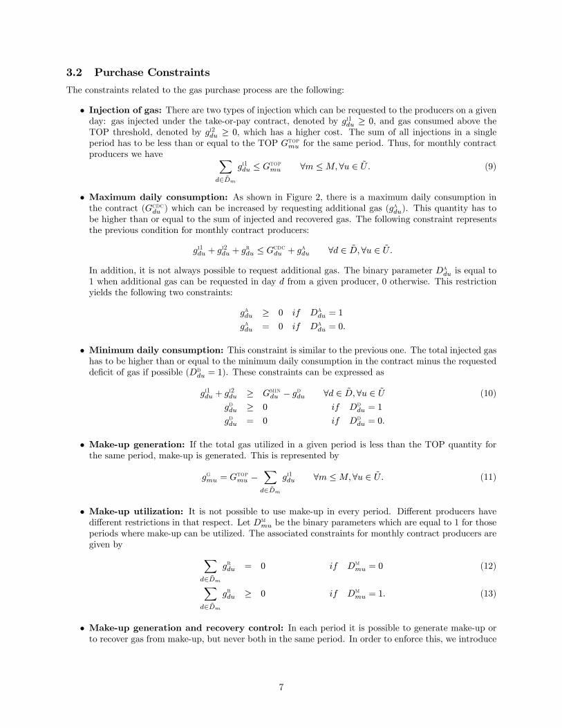
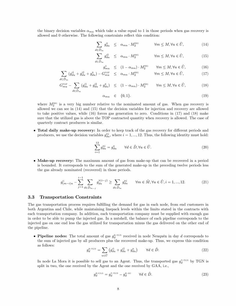
• Make-up recovery: The maximum amount of gas from make-up that can be recovered in a periodis bounded. It corresponds to the sum of the generated make-up in the preceding twelve periods lessthe gas already nominated (recovered) in those periods.

gg(m−i)u −i−1Xj=1

Xd∈Dm−j

gr(i−j)du ≥

Xd∈Dm

gridu ∀m ∈ M,∀u ∈ U , i = 1, ..., 12. (21)

3.3 Transportation Constraints

The gas transportation process requires fulfilling the demand for gas in each node, from end customers inboth Argentina and Chile, while maintaining linepack levels within the limits stated in the contracts witheach transportation company. In addition, each transportation company must be supplied with enough gasin order to be able to pump the injected gas. In a nutshell, the balance of each pipeline corresponds to theinjected gas on one end less the gas utilized for transportation minus the gas delivered on the other end ofthe pipeline.

• Pipeline nodes: The total amount of gas gr-tgnd received in node Neuquén in day d corresponds tothe sum of injected gas by all producers plus the recovered make-up. Thus, we express this conditionas follows:

gr-tgnd =Xu∈U

¡gi1du + g

i2du + g

rdu

¢∀d ∈ D. (22)

In node La Mora it is possible to sell gas to an Agent. Thus, the transported gas gt-tgnd by TGN issplit in two, the one received by the Agent and the one received by GAA, i.e.,

gr-gaad = gt-tgnd − gr-agd ∀d ∈ D. (23)

8

Next, in node Frontera, the received gas by GAC is equivalent to the transported (or delivered) gas byGAA, i.e.,

gr-gacd = gt-gaad ∀d ∈ D, (24)

and finally, the received gas gr-mgd in node Citygate (Metrogas) is equivalent to the transported gas byGAC. Thus,

gr-mgd = gt-gacd ∀d ∈ D. (25)

• Pipelines’ linepack: As mentioned above, a proportion Mb-tgn of the received gas is used to pumpit through the pipeline. Thus, the linepack in TGN is given by the delivered gas minus the receivedgas minus the utilized gas for transportation, as follows:

glpdtgn = gt-tgnd − (1−Mb-tgn) gr-tgnd ∀d ∈ D. (26)

If glp-tgnd > 0 then Metrogas owes gas to the transportation company TGN. Otherwise, TGN owes itto Metrogas. We can similarly define the linepack gas for pipelines GAA and GAC as follows:

glpdgaa = gt-gaad − (1−Mb-gaa) gr-gaad ∀d ∈ D, (27)

glpdgac = gt-gacd − (1−Mb-gac) gr-gacd ∀d ∈ D, (28)

where Mb-gaa and Mb-gac are the proportions of gas used as fuel to transport the gas through thepipeline.

• Gas sale to the Agent: The maximum amount of gas that can be sold to the agent in node LaMora, every day, is restricted by the Agent’s demand Gagd as shown in the following constraint:

gr-agd =Xu∈U

gr-agdu · Gagd ∀d ∈ D. (29)

Just for completeness it is worth to mention that the gas received from quarterly contract producers hasan additional constraint. It cannot exceed a given proportion of the maximum monthly consumption.

• Gas sale at Citygate: The daily gas sales to the end customers in Chile is given by both firm (Dfdc)

and interruptible (didc) demand, and should be fulfilled with the received gas gr-mgd by Metrogas, i.e.,

gr-mgd =Xc∈C

(Dfdc + d

idc) ∀d ∈ D. (30)

In addition, interruptible gas sales to each customer are bounded by their demand Di-maxdc , which is a

parameter, so thatdidc · D

i-maxdc ∀d ∈ D, c ∈ C. (31)

Interruptible gas can only be sold in certain days (when Dintdc = 1), so we add the following constraints

to take that into account:

didc = 0 if Dintdc = 0 (32)

didc ≥ 0 if Dintdc = 1. (33)

• Transportation capacity: Capacity is a big issue. In order to model it, two cases are considered.The cases are when demand (firm and interruptible) go beyond the threshold, which is a big portionof the MDQ, and when demand is less than this threshold. To characterize these cases we let Dvtx

d tobe equal to 0 for all days d ∈ D such thatX

c∈C(Df

dc +Di-maxdc ) ≥MtolGmdqdk ∀d ∈ D, k = gac, (34)

and to be equal to 1 otherwise. The parameter Mtol represents the percentage of GasAndes Chile’sMDQ, which is the mentioned threshold.

9

Case Dvtxd = 0: In this case it is known in advance that the demand is high. For that reason, the

LDC could order gas in advance using four main sources: AOG, UOG, interruptible gas, and deliverydeficiency gas. It is important to recall that the unauthorized overrun gas is divided in three sections.The higher the overrun, the higher the fine rate. The set of constraints associated with the first pipelinein the network, TGN, is given by:

gt-tgnd · (1 +Gaogdk )Gmdqdk + gdddk + g

idk +

P3i=1 g

uogi0dk (35)

0 · guog10dk · (gr-agd + gr-gaad )Muog-10dk

0 · guog20dk · (gr-agd + gr-gaad ) (Muog-20dk −Muog-1

0dk )

0 · guog30dk

for all ∀d ∈ D and k =tgn. The model considers very similar constraints for the other two pipelines,gaa and gac.

Case Dvtxd = 1: In this case the demand is below the committed amount of gas in the contract, so

there is no need to use gas from alternatives sources. Just in case, there is always a chance of usingUOG, which is by far the most expensive choice. The set of constraints are similar to the previousones except for the first one in (35), as shown here:

gt-tgnd · gr-gaad + gr-agd +P3i=1 g

uogi1dtgn ∀d ∈ D. (36)

• Delivery deficiency usage: The Delivery Deficiency (DD) can only be used in those periods whereit is allowed by the transportation company, i.e.,

gdddk = 0 if Ddddk = 0 (37)

gdddk ≥ 0 if Ddddk = 1 (38)

for all d ∈ D and k ∈ T , where T = {tgn, gaa, gac}.

• Delivery deficiency nomination: Total delivery deficiency cannot exceed the maximum availableto the corresponding transportation company, i.e.,X

d∈Dgdddk · G

ddk ∀k ∈ T . (39)

• Daily level of linepack unbalance: Positive or negative daily linepack unbalances are subjectto fines, which depend upon the section in the pipeline where the unbalance occurs. The positiveunbalance cannot exceed a threshold which corresponds to a fraction of the MDQ. Any unbalanceabove it will be subject to a fine. Thus,

glpdk · Mlp-dpdk Gmdqdk +

4Xi=1

glp-dpidk (40)

0 · glp-dp1dk ·Mlp-dp1dk Gmdqdk

0 · glp-dp2dk · (Mlp-dp2dk −Mlp-dp1

dk )Gmdqdk

0 · glp-dp3dk · (Mlp-dp3dk −Mlp-dp2

dk )Gmdqdk

0 · glp-dp4dk

for all d ∈ D and transportation company k ∈ T . For the negative daily linepack unbalance case wehave analogous conditions:

−glpdk · Mlp-dndk Gmdqdk +

4Xi=1

glp-dnidk (41)

0 · glp-dn1dk ·M lp-dn1dk Gmdqdk

0 · glp-dn2dk · (Mlp-dn2dk −Mlp-dn1

dk )Gmdqdk

0 · glp-dn3dk · (Mlp-dn3dk −Mlp-dn2

dk )Gmdqdk

0 · glp-dn4dk

10

for all d ∈ D and k ∈ T .

• Cumulative level of linepack unbalance: Monthly linepack unbalances are also considered. Thisconstraint is pretty similar to the previous one. There are two changes. First, instead of lp-dp orlp-dn we have lp-cp or lp-cn respectively. Second, the left hand side of (40) considers the cumulativelinepack until day d, i.e., X

{d:d�d,d∈D}glpdk·Mlp-cp

dk Gmdqdk +4Xi=1

glp-cpidk (42)

for all d ∈ D and k ∈ T .

3.4 Boundary Conditions

Information from previous days has to be maintained because of the boundary conditions of the model. Theinjected-gas levels gi1du and g

i2du, the recovered gas g

rdu, the additional gas g

adu, and the deficit gas g

ddu, are

gathered from the database for all producers and all days prior to the current day when the model is beingoptimized (for all u ∈ U and d ∈ Dp).Analogously, on the transportation side, the received gas gr-kd , the transported gas gt-kd , the linepack gas

glp-kd , and the unauthorized overrun gas guogi·dk , have to be gathered from the database for all k ∈ T andd ∈ Dp.

4 Implementation at MetrogasThe model described above was the basis for a DSS for Metrogas, an LDC formed in 1994 for distributingnatural gas to residential, commercial, and industrial customers in Chile. Since it began operations in 1997,it has grown very fast. At the end of 2000 it distributed natural gas to over 200.000 residential customers,which makes it the largest LDC in Chile.The DSS we implemented for Metrogas, was designed to support the daily decision of how much to

request from each of the gas producers and how to transport it. This decision was transmitted by fax in theeve of the day when the injection was to be carried out. This fax (see Appendix A) also took into accountany adjustment that were necessary due to differences between the amounts requested and those effectivelydelivered. The amount of information required to support these decisions is very large, and handling thecorresponding data was one of the main problems for the decision makers. Therefore, it was important thatthe model design supported data management as much as possible.Although the mixed-integer programming model that needed to be solved had 224,881 variables, 80 of

which were integer, and 80,379 constraints, it was solved to optimality in less than 2 hours in a personalcomputer, which was acceptable to the decision-makers. The size of the problem resulted from having dailydecision variables over a planning horizon of five years. We considered the alternative of using monthlydecision variables for more distant periods, in order to reduce the total number of continuous decisionvariables. In addition, some auxiliary daily decision variables required by the decision-makers could beaggregated at a monthly level. However, reducing the total number of continuous variables had little impacton the solution time, compared to the impact of the total number of integer variables. Since the solutiontime was reasonably short, we focused instead on making the operation and maintenance of the DSS as easyas possible. Periodically updating a significant amount of data, as better estimates became available andoperational conditions changed, was a nontrivial task for the daily operation of the DSS.In order to test the model, we solved it with different data sets. Since checking the validity of the solution

was quite difficult for the complete data set, we used smaller versions of the model. For example, we used a16 period data set, with 4 periods per month, in order to see how the model handled contracts with differentlevels of TOP. Figure 4 shows the main decision variables, assuming a relatively low level of TOP and givenan initial level of generated makeup of 4000. VINY1M was the variable for the level of gas injected underthe TOP level, VINY2M was the variable for the gas injected over the TOP level, and VMUPRM was thevariable for makeup recovered gas. The solution shows how the model first uses the injection under TOPuntil the level of 5000 is achieved, then it makes use of previously generated makeup, and lastly of injection

11

Figure 4: Solution for Take-or-Pay of 5000

of gas over TOP. In Figure 5, it can be seen that with a higher level of TOP, the model drastically reducesthe amount of gas over the TOP level, which is more expensive.In an another test, we studied how the model handled the aging of generated makeup. The results shown

in Figure ?? correspond to a data set with only one day per month, where the generated makeup expiresafter 4 months. The planning horizon was 4 years plus 1 year of historic data. The figure shows the solutionfor the first 18 months, which is the most relevant part. Note that as the makeup stock gets older, it isshown in a darker color. In month 4 the model makes use of the makeup generated the previous month.In month 6, more makeup is generated and kept for 4 months until it expires. The same happens with themakeup generated in month 8, which is also lost. However, the makeup generated in month 13 is entirelyused during the next three months.The solution generated by the system, using real data, minimized the cost of supplying the required gas

to residential customers and interruptible service. The solution optimizes the use of linepack unbalances andmake-up generation of the different types of contracts. Seasonal patterns were clearly discernible. Duringthe summer, when residential demand diminishes, interruptible service increases. Also, since we assumed astrong growth in demand, the solution tends to generate make-up in the first part of the planning horizon soit can be recovered in the latter part. During the first part of the planning horizon, almost no additional gaswas required. However, towards the end of the planning horizon, there is significant purchase of additionalgas, especially during the winter.The model was specified in SML (Geoffrion, 1992), which is a modeling language based on the structured

modeling approach developed by Geoffrion (1989). SML turned out to be a very good choice considering thecomplexity of the model and the need for many revisions. We used WIN/SM to build the OBDSS. WIN/SMis a software that has a specialized editor for specifying the model in SML, tools for managing data, andan interface to interact with a commercial solver. This system is described in more detail in (Maturanaet al., 2004). The use of WIN/SM enabled us to generate, in a very short time, many versions of the system.This allowed us to quickly test the model and verify the solutions. We developed and tested twelve differentversions of the model, not counting minor variations.

12

Figure 5: Solution for Take-or-Pay of 7000

Figure 6: Monthly Makeup Generation and Recovery

13

5 The Robust Optimization ExtensionThe deterministic gas purchasing and transportation optimization model described above can be used toanalyze different future demand scenarios. For example, it can be solved for every scenario we wish toconsider, generating a different optimal solution for each one. If these optimal solutions are similar, at leastfor the first few days in the rolling planning horizon, decision makers can use them as a basis for theirdecisions. Otherwise, they can either choose the solution from one of the scenarios or generate a differentone by combining several of these solutions, in which case they can evaluate it under the different scenarios.They can also apply classical sensitivity analysis to this solution. According to Avery et al. (1992), scenarioanalysis gives good results in practice and its use is also well accepted by the LDC’s.However, since the approach described above may not work very well in some cases, we explored using a

robust optimization model for dealing with demand uncertainty. The robust optimization approach can bedescribed as finding a solution whose objective value is sufficiently close to that of the optimal solution foreach scenario (Mulvey et al., 1995). Each of these scenarios has a certain probability of occurrence. In themodel we analyzed (Ortiz, 2001), the here and now decision variables are the daily gas purchase decisionvariables over the entire planning horizon. The recourse variables, which depend on the scenarios, aremake-up generation and recovery, linepack unbalances, unsatisfied interruptible demand, and the 0-1 integervariables, which prevent, at each period, the recovery of make-up gas generated in the same period, overthe entire planning horizon. The objective of the robust optimization model is to maximize the differencebetween the total income and the total expected recourse cost, which is the expected value of the costsassociated to recourse variables for each scenario.To explore the usefulness of implementing a robust optimization model of the real problem, we analyzed

a model with a reduced number of scenarios. We used variations of the historic weather and temperaturerecords to generate twenty eight demand scenarios over a time horizon of three years, considering only twoseasons per year.Based on these scenarios, we computed the Wait and See value (WS) and the Expected Expected Value

(EEV). WS is obtained by solving the deterministic model for each scenario and computing the expectedvalue of the optimal values of these models. EEV is obtained by solving the robust model, with the here andnow variables fixed at the values of the optimal solution of the deterministic model solved for the averagescenario. For the given scenarios, we obtained an EEV of $39,765,915 and a WS of $42,799,682. Since theoptimal value of the robust optimization model must fall within the interval defined by these two values, thedifference (WS-EEV) gave us an upper bound of $3,033,767 on the additional benefit that may be obtainedby solving the robust model instead of the deterministic one. However, it was not possible to solve the robustmodel within a reasonable solution time, even for this reduced number of scenarios.In order to solve a more realistic model we require a more efficient solution method, such as a scenario

decomposition approach, in order to take advantage of the deterministic MIP structure, for example usingAugmented Lagrangean Relaxation techniques (Contesse & Guignard, 1995).

6 Concluding RemarksIn this work we presented a mixed-integer programming model that is the basis for an OBDSS we developedfor a Chilean local natural gas distribution company. The model takes into account all the complexities ofthe purchasing and transportation contracts to help optimize the company’s daily decisions in the absenceof local storage facilities. The model is quite large in order to represent the daily, monthly, quarterly, andyearly conditions specified in the contracts. We also discuss an extension for the case when demand scenariosare used to deal with demand uncertainty.The model we developed is one of the largest and most detailed mixed-integer programming model we have

seen that has been solved to optimality. It includes several innovations, such as the treatment of make-upgeneration and recovery, the aging of generated make-up, the use of linepack to handle demand fluctuation,and the inclusion of fines for different types of deficits and overruns. Despite the size and complexity of themodel, it turned out to be relatively easy to solve, thanks to the relatively small number of integer variablesand its particular structure.The main difficulties for developing the model were validating it and collecting all the data it required.

In the validation, the use of the tools based on structured modeling (Maturana et al., 2004) was very helpful,

14

since it allowed us to quickly generate and run new versions of the model. We had to develop and test manyversions of the model before we were satisfied that the conditions of the contracts were adequately takeninto account. The use of SML was also important in dealing with many versions of a very large and complexmodel.Although the model was developed to support operational decisions, it can also be used to help in

negotiating new contracts by helping to quantify the effect that certain conditions, such as the amount ofTOP, will have on the profits of the company.

ReferencesAvery, William, Gerald Brown, John Rosenkranz, and Kevin Wood. (1992). Optimization of Purchase,

Storage, and Transmission Contracts for Natural Gas Utilities. Operations Research, 40(3), 446—462.

Chin, Louis and Thomas Vollmann. (1992). Decision Support Models for Natural Gas Dispatch. Transporta-tion Journal, 32(2), 38—45.

Contesse, Luis and Monique Guignard. (1995). A Proximal Augmented Lagrangean Relaxation for Linear andNonlinear Integer Programming. Tech. rept. 95-03-06. Dept. of OPIM, The Wharton School, Universityof Pennsylvania.

De Wolf, Daniel and Yves Smeers. (2000). The Gas Transmission Problem Solved by an Extension of theSimplex Algorithm. Management Science, 46(11), 1454—1465.

Gazmuri, Pedro and Sergio Maturana. (2001). Developing and Implementing a Production Planning DSSfor CTI Using Structured Modeling. Interfaces, 31(4), 22—36.

Gazmuri, Pedro, Sergio Maturana, Fernando Vicuña, and Luis Contesse. (1993). Diseño de un Generador deSistemas Computacionales para la Optimización de Procesos Productivos. FONDEF Proposal. PontificiaUniversidad Católica de Chile.

Geoffrion, Arthur. (1989). The Formal Aspects of Structured Modeling. Operations Research, 37(1), 30—51.

Geoffrion, Arthur. (1992). The SML Language for Structured Modeling. Operations Research, 40(1), 38—75.

Guldmann, Jean-Michel and Fahui Wang. (1999). Optimizing the Natural Gas Supply Mix of Local Distri-bution Utilities. European Journal of Operational Research, 112, 598—612.

Knowles, Thomas and John Wirick, Jr.. (1998). The Peoples Gas Light and Coke Company Plans GasSupply. Interfaces, 28(5), 1—12.

Levary, Reuven and Burton Dean. (1980). A Natural Gas Flow Model Under Uncertainty in Demand.Operations Research, 28(6), 1360—1374.

Maturana, Sergio, Juan-Carlos Ferrer, and Francisco Barañao. (2004). Design and Implementation of anOptimization-Based Decision Support System Generator. European Journal of Operational Research,154(1), 170—183.

Mulvey, John, Robert Vanderbei, and Stavros Zenios. (1995). Robust Optimization of Large-scale Systems.Operations Research, 43(2), 264—281.

Murphy, Frederic, Reginald Sanders, Susan Shaw, and Richard Trasker. (1981). Modeling Natural GasRegulatory Proposals Using the Project Independence Evaluation System. Operations Research, 29(5),876—902.

O’Neill, Richard, Mark Willard, Bert Wilkins, and Ralph Pike. (1979). A Mathematical Programming Modelfor Allocation of Natural Gas. Operations Research, 27(5), 857—872.

15

Ortiz, Alejandro. (2001). Optimización bajo Condiciones de Incertidumbre: Aplicación en la Compra de GasNatural. M.Sc. thesis, Engineering School, Pontificia Universidad Católica de Chile.

Sun, Chi Ki, Varanon Uraikul, Christine Chan, and Paitoon Tontiwachwuthikul. (2000). An IntegratedExpert System/Operations Research Approach for the Optimization of Natural Gas Pipeline Operations.Engineering Applications of Artificial Intelligence, 13, 465—475.

A Daily Gas Nomination Form

Nomination fax

16

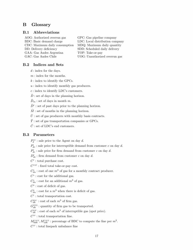
B Glossary

B.1 AbbreviationsAOG: Authorized overrun gas GPC: Gas pipeline companyBDC: Basic demand charge LDC: Local distribution companyCDC: Maximum daily consumption MDQ: Maximum daily quantityDD: Delivery deficiency SDD: Scheduled daily deliveryGAA: Gas Andes Argentina TOP: Take-or-payGAC: Gas Andes Chile UOG: Unauthorized overrun gas

B.2 Indices and Sets

d : index for the days.

m : index for the months.

k : index to identify the GPCs.

u : index to identify monthly gas producers.

c : index to identify LDC’s customers.

D : set of days in the planning horizon.

Dm : set of days in month m.

Dp : set of past days prior to the planning horizon.

M : set of months in the planning horizon.

U : set of gas producers with monthly basis contracts.

T : set of gas transportation companies or GPCs.

C : set of LDC’s end customers.

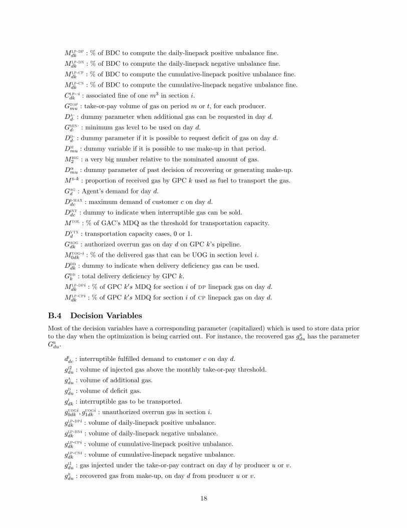
B.3 Parameters

P agd : sale price to the Agent on day d.

P idc : sale price for interruptible demand from customer c on day d.

P fdc : sale price for firm demand from customer c on day d.

Dfdc : firm demand from customer c on day d.

Cp : total purchase cost.

Ctop : fixed total take-or-pay cost.

Cgdu : cost of one m3 of gas for a monthly contract producer.

Ca : cost for the additional gas.

Cadu : cost for an additional m3 of gas.

Cd : cost of deficit of gas.

Cddu : cost for a m3 when there is deficit of gas.

Ct : total transportation cost.

Cbdcdk : cost of each m3 of firm gas.

Gmdqdk : quantity of firm gas to be transported.

Cpspdk : cost of each m3 of interruptible gas (spot price).

Ctf : total transportation fine.

Muogi0dk ,M

uogi1dk : percentage of BDC to compute the fine per m3.

Clf : total linepack unbalance fine

17

Mlp-dpdk : % of BDC to compute the daily-linepack positive unbalance fine.

Mlp-dndk : % of BDC to compute the daily-linepack negative unbalance fine.

Mlp-cpdk : % of BDC to compute the cumulative-linepack positive unbalance fine.

Mlp-cndk : % of BDC to compute the cumulative-linepack negative unbalance fine.

Clp-·idk : associated fine of one m3 in section i.

Gtopmu : take-or-pay volume of gas on period m or t, for each producer.

Da·d· : dummy parameter when additional gas can be requested in day d.

Gmin·d· : minimum gas level to be used on day d.

Dd·d· : dummy parameter if it is possible to request deficit of gas on day d.

Dmmu : dummy variable if it is possible to use make-up in that period.

Mbig2 : a very big number relative to the nominated amount of gas.

Dαmu : dummy parameter of past decision of recovering or generating make-up.

Mb-k : proportion of received gas by GPC k used as fuel to transport the gas.

Gagd : Agent’s demand for day d.

Di-maxdc : maximum demand of customer c on day d.

Dintdc : dummy to indicate when interruptible gas can be sold.

Mtol : % of GAC’s MDQ as the threshold for transportation capacity.

Dvtxd : transportation capacity cases, 0 or 1.

Gaogdk : authorized overrun gas on day d on GPC k’s pipeline.

Muog-i0dk : % of the delivered gas that can be UOG in section level i.

Ddddk : dummy to indicate when delivery deficiency gas can be used.

Gddk : total delivery deficiency by GPC k.

Mlp-dpidk : % of GPC k0s MDQ for section i of dp linepack gas on day d.

Mlp-cpidk : % of GPC k0s MDQ for section i of cp linepack gas on day d.

B.4 Decision Variables

Most of the decision variables have a corresponding parameter (capitalized) which is used to store data priorto the day when the optimization is being carried out. For instance, the recovered gas grdu has the parameterGrdu.

didc : interruptible fulfilled demand to customer c on day d.

gi2du : volume of injected gas above the monthly take-or-pay threshold.

gadu : volume of additional gas.

gddu : volume of deficit gas.

gidk : interruptible gas to be transported.

guogi0dk , guogi1dk : unauthorized overrun gas in section i.

glp-dpidk : volume of daily-linepack positive unbalance.

glp-dnidk : volume of daily-linepack negative unbalance.

glp-cpidk : volume of cumulative-linepack positive unbalance.

glp-cnidk : volume of cumulative-linepack negative unbalance.

gi1du : gas injected under the take-or-pay contract on day d by producer u or v.

grdu : recovered gas from make-up, on day d from producer u or v.

18

ggmu : generated make-up on period m or t.

αmu : binary variable equal to 1 when it is allowed to recover gas.

gridu : recovered gas on day d from make-up of i previous periods.

gr-kd : gas received by GPC k on day d.

gr-agd : gas received by the Agent on day d.

gr-mgd : gas received by the Metrogas on day d.

gt-kd : gas transported by GPC k on day d.

glpdk : GPC k0s linepack on day d, positive or negative volume of gas.

gr-agdu : gas received by the Agent on day d from producer u.

gdddk : delivery deficiency gas by GPC k on day d.

guogi·dk , guogi·dk : unauthorized overrun gas in section level i on day d GPC k.

glp-dpidk : section i0s dp linepack gas on day d from GPC k.

19