A Mixed Integer Programming Formulation for the ... · PDF fileA Mixed Integer Programming Formulation for the Heterogeneous Fixed Fleet Open Vehicle Routing Problem Majid Yousefikhoshbakhta,*,

A Mixed Integer Programming Formulation for the Heterogeneous Fixed Fleet Open Vehicle Routing Problem

Majid Yousefikhoshbakhta,*, Frazad Didehvarb, Farhad Rahmatic

aAssistant Professor, Department of Mathematics, Faculty of Science, Bu-Ali Sina University, Hamedan, Iran bAssistant Professor, Department of Mathematics and Computer Science, Amirkabir University of Technology, Tehran, Iran cAssociate Professor, Department of Mathematics and Computer Science, Amirkabir University of Technology, Tehran, Iran

Received 27 January, 2014; Revised 21 February, 2015; Accepted 04 March, 2015

Abstract

The heterogeneous fixed fleet open vehicle routing problem (HFFOVRP) is one of the most significant extension problems of the open vehicle routing problem (OVRP). The HFFOVRP is the problem of designing collection routes to a number of predefined nodes by a fixed fleet number of vehicles with various capacities and related costs. In this problem, the vehicle doesn’t return to the depot after serving the last customer. Because of its numerous applications in industrial and service problems, a new model of the HFFOVRP based on mixed integer programming is proposed in this paper. Furthermore, due to its NP-hard nature, an ant colony system (ACS) algorithm was proposed. Since there were no existing benchmarks, this study generated some test problems. From the comparison with the results of exact algorithm, the proposed algorithm showed that it can provide better solutions within a comparatively shorter period of time. Keywords: Open Vehicle Routing Problem, Heterogeneous fleet, Ant Colony System, Exact Algorithm, Mixed Integer programming.

1. Introduction

In today's commerce world, freight transportation plays a significant role in logistics and supply chain management. It supports and makes most other social and economic activities possible. That is why many companies are giving special attention to the transportation costs of goods in order to minimize their expenses. Companies try to reduce transportation costs by using rational manners and effective tools. Consequently, Capacitated Vehicle Routing Problem (CVRP) and its versions have been receiving much attention by researchers and scientists (Yousefikhoshbakht et al., 2014). The CVRP is the basic version of the VRP, where all customers are delivery customers, the demands are known, all vehicles are identical and they belong to the same central depot. The imposed constraints are related to the capacity of the vehicles, may also be restricted in the total distance. It can travel and all customers must be served by a single route. In this problem, the objective is to find a set of delivery routes satisfying these requirements and giving minimal total travel cost. To make CVRP models more realistic and applicable, there are many varieties of the VRP obtained by adding constraints to the basic model. Examples of such

extensions are VRP with Time Windows (VRPTW) (Tzeng et al., 1997), VRP with backhauls (VRPB) (Popovic, 1995), Stochastic VRP (SVRP) (Teodorovic et al., 1995), Multi-depot VRP (MDVRP) (Geetha et al., 2012), VRP with simultaneously Pickup and Delivery (VRPSPD) (Yousefikhoshbakht et al., 2014), Split Delivery VRP (Ozfirat et al., 2010), Open VRP (OVRP) (9) and so on with different constraints (Yousefikhoshbakht et al., 2012).

Nowadays, many enterprises contract their physical distribution tasks to third party logistics companies. These outsourcing carriers are paid on the basis of fixed costs and traveling distances of the ‘for-hire’ vehicles. Therefore, the vehicle starts at the depot and terminate at one of the customers after servicing the last customer on its route. This problem is regarded as an OVRP in which the route of each vehicle is a Hamiltonian path. At first sight, having open routes instead of closed ones looks like a minor modification. Indeed, if travel costs are asymmetric, there is essentially no difference between the open and closed versions. In other words, to transform the open version into the closed one, it suffices to set the cost to zero for traveling from any customer to the depot. However, if travel costs are symmetric, things are more subtle. Indeed, the open VRP turns out to be more general than the closed VRP, in the sense that any closed version

* Corresponding author Email address: yousefikhoshbakht@ basu.ac.ir

Journal of Optimization in Industrial Engineering 18 (2015) 37-46

37

on n customers can be transformed into an open version on n customers, but there is no transformation in the reverse direction.

The OVRP is characterized by the following: a fleet of predefined vehicles that start to move simultaneously from the depot but not come back to the depot after visiting customers are used to serve customers distributed geographically in the area. The capacity of each vehicle is called Q. A customer requires a given shipment to be picked up during a single visit by a vehicle. The objective is to design a set of minimum cost routes to serve all customers so that the load on a vehicle is below vehicle capacity Q at each point on the route. In other words, a solution to the OVRP consists of a set of Hamiltonian paths, rather than Hamiltonian cycles. The problem of finding the best Hamiltonian path for each set of customers assigned to a vehicle is NP-hard (Syslo et al. 1983). Hence OVRP is also NP-hard (Brandaõ, 2004). An example of a single solution consisting of a set of routes constructed for an OVRP is presented in Figure 1.

Fig. 1. A solution of OVRP

Brandaõ (2004) observes that Schrage was the first to raise the problem in an article dedicated to the description of realistic routing problems (Schrage, 1981). However, the earliest work which addressed solving the OVRP seems to have been introduced in 2000 by Sariklis and Powell who did not impose a maximum route length. Instead, they developed a heuristic algorithm based on two phases including cluster-first route-second (Sariklis et al., 2000). In the first phase, customers are assigned to vehicles, taking into account the capacity constraint, while attempting to create a minimum number of vehicles. Then, total travel cost is reduced by applying some given rules for moving customers among clusters. In the second phase, a minimum spanning tree is created for each cluster through a set of operations and then it is transformed into an open route which is short as much as possible.

Exact branch-and-cut approach has been proposed by Letchford, et al., (2007), addressing the capacitated problem with no distance constraints and no empty routes

allowed (i.e., exactly m vehicles must be used). Besides, the authors provide an OVRP integer programming formulation together with some valid inequalities. The proposed algorithm is capable of solving optimality small to medium-sized OVRP instances. When the size of the problem increases, the complexity of the problem also increases rapidly. Consequently, they provide lower bounds for the large scale instances which are helpful for assessing the effectiveness of approximate solution methodologies.

Although there are other exact algorithms which investigate fewer solutions, it is almost impossible even in such cases to find an optimum solution within a satisfactory time limit. Therefore, exact algorithms are not capable of solving problems for large dimensions. On the other hand, heuristics and meta-heuristics are thought to be more efficient for complex OVRPs and have become very popular for researchers. Different algorithms have been developed to solve the OVRP base on heuristic and meta-heuristic such as tabu search (Fu et al., 2005), record-to-record travel algorithm (Li et al., 2007), neighborhood search algorithm (Fleszar et al., 2008), ant colony optimization (ACO) (Yousefikhoshbakht et al., 2012), and particle swarm optimization (MirHassani et al. 2011).

An efficient tabu search was proposed by Brandeo (2004) in which the neighborhood structure is defined by insertions and swaps between different routes. It is noted that in this algorithm, several features from previous tabu search implementations for the classical VRP are used. Furthermore, infeasibilities in intermediate solutions are managed through penalizing the objective function by two penalty terms including for capacity violation and the for route length violation. Besides, Fu et al. (2005) and Fu et al. (2006) also present a tabu search algorithm. In this algorithm, a farthest first heuristic is used for initial solution. Furthermore, the two-interchange generation mechanism within the same route or between two routes are applied, but with a combination of vertex reassignment, vertex swap, 2-opt and ‘tails’ swap. A variant of the VRP in which the objective is to minimize the total distance covered was offered by Tarantilis, et al. (2005). In this paper attempting directly to minimize the number of vehicles and imposing an upper limit on route length, were not considered. Their solution algorithm is a single-parameter meta-heuristic method that exploits a list of threshold values to guide intelligently a local search based on a variety of edge and node exchanges.

Also, Pisinger et al. (2007) offer an adaptive large neighborhood search algorithm. In this proposed algorithm, customers can be removed at random from the solution and then reinserted in the cheapest possible route. Various removal and insertion heuristics can be used to diversify and intensify the search for this algorithm, but moving from one solution to the next is carried out within a simulated annealing framework.

Because the company may contract its delivery activities to a number of outsourcing carriers which may

Majid Yousefikhoshbakht et al./ A Mixed Integer Programming...

38

own a heterogeneous fleet of vehicles available for hiring, considering a fleet of homogeneous vehicles is not practical in the VRP. Hence, the heterogeneous fleet vehicle routing problem has been investigated by many scientists and researchers (Li et al., 2010). Moreover, if in this problem, the number of vehicles available to perform the delivery is considered limited and the vehicles have different capacities, fixed costs and variable costs per unit distance, it is called heterogeneous fixed fleet open vehicle routing problem (HFFOVRP).

The HFFOVRP can be converted into an open vehicle routing problem (OVRP) and heterogeneous fixed fleet vehicle routing problem (HFFVRP). In more detail, the OVRP can be obtained from HFFOVRP by removing the constraint of vehicle heterogeneity. Similarly, HFFOVRP by removing the constraint of vehicle heterogeneity of Hamiltonian path can be converted to a VRP with a heterogeneous fixed fleet. Since OVRP and HFFVRP are NP-hard combinatorial optimization problems (Cao et al., 2010), The HFFOVRP is an NP-hard problem.

Recently, most of the research effort aimed at solving the NP-hard problems, have focused on the development of various meta-heuristic algorithms. A meta-heuristic can be defined as a top-level general strategy which guides other heuristics to search for good solutions in feasible space. Most of the VRP meta-heuristic algorithms are based on some construction and improvement heuristics, i.e., they use the so-called local search principle (Reimann et al., 2004). The aim of this paper is to apply the exact algorithm and ant colony system (ACS) to deal with the new variant of the VRPs, HFFOVRP. To reach this goal, first we propose a mixed integer programming named as node based formulation and then obtained results by the CPLEX 12.4 and ACS are compared together for some instances. The rest of this paper is organized as follows. In Section 2, a proposed mixed integer model is described. In Section 3, the details of the proposed approach are introduced. Experimental evaluation of this algorithm is reported in Section 4. Finally, we report the computational results of the proposed algorithm based on the generated benchmark problems. In Section 5, we conclude this paper and discuss some possible research extensions in future work.

2. Problem Description and Formulation

2.1. Problem definition

From a graph theoretical point of view, we can define the HFFOVRP as follows. Let G = (V, E) be an undirected connected graph with V 0,1,..., n as the set of

vertexes and the set of arcs E (i, j):0 i, j n (if the graph is not complete, we can compensate the lack of each arc with the arc that has infinite size). Node 0 is the depot and the customer set C consist of n customers, i.e.

C 1, 2, ..., n . A nonnegative cost ijd (

iid 0, 0 i n ) associated with each arc i j(v , v ) E.

0v represents the depot and each vertex iv C is a

customer with a non-negative demand ip . The available fleet consists of K different type vehicles located at the depot and the number of available vehicles of each type is fixed and equal to kn . A capacity kQ , a fixed cost kf ,

variable cost k is associated with each type of vehicle k

and. k is cost per unit of distance corresponding to each

vehicle type k. Hence, kij ij kc d represents the cost

of the travel from customer i to j with a vehicle of type k. The HFFOVRP deals with finding the minimum total transportation cost including the fixed and variable cost for a fleet of vehicles which start and end at the depot, so that the following constraints are taken into account: The total load of each vehicle cannot exceed the

capacity of the corresponding vehicle type. The number of vehicles of type k used cannot exceed

kn . The demand of each customer is satisfied by exactly

one vehicle in only one visit.

2.2. Problem formulation

We present following mathematical formulation for HFFVRP using variables and ijy where, k

ijx take the value 1 if a vehicle of type k travels directly from customer i to customer j, and 0 otherwise; denotes the route. The flow variables ijy specify the quantity of goods that a vehicle k is carrying when leaves customer i to service customer j.

K n K n nk k k

k 0 j ij ijk 1 j 1 k 1 i 0 j 0

Min f x c x

(1)

subject to K n

kij

k 1 i 0x 1 j 1, 2,..., n

(2)

K nkij

k 1 j 1

x 1 i 1,2,..., n

(3)

n nk kij ji

i 1 i 1

0 x x 1

j 1,2,..., n , k 1, 2,..., K

(5)

nk0 j k

j 1

x n , k 1, 2,..., K

(6)


39

K n K nk kij ji j

k 1 i 0 k 1 i 0

y y p ,

j 1, 2,..., n

(7)

k k kj ij ij k i ijp x y (Q p )xi, j 0,1,..., n ,i j, k 1, 2,..., K

(8)

nki0

j 1

x 0, k 1, 2,..., K

(9)

k

ijx 0,1 i, j 0,1,..., n , i j , k 1, 2,..., K (10) kijy 0 i, j 0,1,..., n , k 1, 2,...,K (11)

The objective function (1) gives the sum of the total fixed cost of the vehicles used plus the total variable routing cost. Constraints (2) mean that only one arc can be entered for each customer; however, constraints (3) show that almost one arc can be exited from each customer. Constraints (4) states that if a vehicle visits a customer, it can remain there or depart from it. The maximum number of vehicles available for each vehicle type is guaranteed by constraints (5). Equality equations (6) insure that the demands of all customers are fully satisfied. Constraints (7) state that the vehicle capacity is never exceeded. Constraints (8) guarantee that there is not any arc from each customer to the depot. Constraints (9) describe that each arc in the network has the value 1 if it is used and 0 otherwise. Finally, Restrictions (10) force the flow to remain non-negative.

3. Solution Method

In this section at first the classic ACO is explained and then modification of EAS as the proposed algorithm is explained in more details.

3.1 Ant Colony Optimization

Studies on real ants show that although ants lack sight, they can find the shortest path from the food sources to the nest by depositing pheromones. In other words, when ants move from one place to another to find the shortest path, they secrete this chemical material both for guiding other ants which are going to exit the nest later and for recognizing the return path to the nest. Therefore, after a few times the route which ants traveled is marked by this chemical material and then more ants by instinct select this shorter path with more probability and much more pheromone remains on this shorter path.

ACO is one of the most important meta-heuristic algorithms used to obtain good enough solutions not found by any effective algorithm yet to hard combinational optimization problems within a reasonable amount of computation time. Dorigo proposed this algorithm and proved its acceptable performance for traveling salesman problem (Dorigo et al., 1992).

It has been applied to several NP-hard combinatorial optimization problems such as quadratic assignment problem (Maniezzo et al., 34), the vehicle routing problem (Bullnheimer et al., 1999), bin packing, stock cutting (Ducatelle et al., 2001) and RNA secondary structure prediction (McMellan, 2006). The inspiring source of ACO is the pheromone trail laying and following behavior of real ants which use pheromones as a communication medium. Similar to ant communication system, ACO is based on the indirect communication of a colony of simple agents called (artificial) ants which communicate by secreting (artificial) pheromone on trails. This experience shows that the simple swarm intelligence, which is used by ants for finding food, can help to solve the hard combinational problems and reach a solution which is very close to the optimal situation.

Since the initial version of ACO called Ant System (AS) was not competitive with other meta-heuristic algorithms of its time for solving small scale TSP instances a large number of authors developed newer and more advanced versions of ACO by modifying the method of updating the local and global pheromones or distributing ants on the nodes. These developments led to more efficient algorithms like EAS (Dorigo et al., 1996), ACS (Bullnheimer et al., 1997) and rank based ant system (RAS) (Dorigo et al., 1997). Furthermore, the application and the efficiency of these algorithms have gained more attention compared to some other meta-heuristic algorithms including GA, Simulated Annealing, etc. Therefore, more sophisticated models of ACO which are used to successfully solve a large number of complex combinatorial optimization problems. Theoretical insights into the algorithm are now becoming available. For ACO convergence proofs, theories and open problems we refer the readers to (Dorigo et al., 2005).

3.2 The proposed Algorithm

ACS is one of the famous versions of the ACO proposed by (Dorigo et al., 1997). This algorithm, although strongly inspired by AS, achieves performance improvements through the introduction of new mechanisms based on ideas not included in the original. ACS as an improved algorithm differs from the previous AS in three main aspects:

(1) The state transition rule provides a direct way to balance between exploration of new edges and exploitation of a priori and accumulated knowledge about the problem.

(2) The global updating rule is applied only to edges which belong to the best ant tour.

(3) While ants construct a solution a local pheromone updating rule (local updating rule, for short) is applied. Updating the pheromone simulates the changes in values of pheromone in any iteration and mainly it is one of the reasons that algorithms are different.

Generally, two operations motivate this updating procedure in ACS algorithm:


40

(1) A new transition rule: this rule is introduced that favors either exploitation or exploration. From node i, the next node j in the route is selected by ant k, among the unvisited nodes k

iJ , according to the following transition rule which shows the probability of each city being visited:

0

arg max {[ ( )] .[ ( )] }

exp( ) ( ) ( )

( ) ( )

exp

ki

ki

ir irr J

kij ij ij

ir irr J

t t

if q q loitationP t t t

t t

Otherw ise loration

(11)

Where

ij(t) : The amount of pheromone on the edge joining nodes i and j

ij(t) : The heuristic information for the ant visibility measure defined as the reciprocal of the distance between node i and node j for the TSP

, : The parameters that determine the relative

importance of the pheromone level ij and the heuristic

search function ij on the edge joining nodes i and j. q: Random number with uniform probability distribution between zero and one [0, 1].

Real variable that determines the relative importance

of the exploitation over the exploration ( 0 10 q ).

It is noted that when q is less than or equal to 0q , the ant employs exploitation to select the next node in its tour, whereas if q exceeds the ant uses probabilistic exploration to select the next node in its tour. (2) The local updating: When the ant moves between nodes i and j, it updates the amount of pheromone on the traversed edge using the formula (12). The effect of local updating is that each time an ant traverses an edge (i, j) its pheromone trail ij is reduced, so that edges becomes less desirable for the ants in future iterations. This encourages an increase in the exploration of edges that have not been visited yet. Local updating helps avoid poor stagnant situations.

0( 1) (1 ). ( ) { ( , ) }ij ij kt t if edge i j T (12) Where

0 : The initial amount of pheromone calculated as 1

0 )( inC n: The number of customers

:iC The cost of the initial tour produced by a construction heuristic such as the Nearest Neighbor heuristic

: A parameter in the range [0, 1] called the evaporation rate that regulates the reduction of pheromone on the edges (3) The global updating: When all ants have generated their tours, the edges belonging to the best tour are updated using the formula (13). It is important to note that global updating adjusts only the pheromone on the edges belonging to the best tour. This encourages ants in future iterations to search in the vicinity of this best tour.

( 1) (1 ). ( ) (1/ ){ ( , ) }

ij ij b

b

t t Cif edge i j T

(13)

Where :bC The cost of the best tour bT has been found since

the start of the algorithm. ACS works on HFFOVRP as follows: m group of ants in which each group has n ants are initially positioned depot. Each ant builds a Hamiltonian path (i.e., a feasible solution to the HFFOVRP) by repeatedly applying the state transition rule. While constructing its tour, an ant also modifies the amount of pheromone on the visited edges by applying the local updating rule. Once all ants have terminated their path, the amount of pheromone on edges is modified again by applying the global updating rule. As was the case in ACS, ants are guided, in building their tours in formula (11), by both exploitation (they prefer to exploit a priori and accumulated knowledge about the problem), and by exploration: A new edge is exploited by algorithm. The pheromone updating rules are designed, so that they tend to give more pheromone to edges which should be visited by ants. The vast amount of literature on ACOs tells us that, a promising approach to obtaining high-quality solutions is to couple a local search algorithm with a mechanism to generate initial solutions. A local search approach starts with an initial solution and searches within neighborhoods for better solutions. In the proposed algorithm, after each group has constructed their solutions, the best groups’ solution is improved by applying a local search. The idea here is that a better solution may have a better chance to find a global optimum. We first apply a local search based on an insert move to the ant (Figure 2), and then apply the swap move (Figure 3). In insert algorithm a node is moved. However, in swap algorithm a node is swapped with another node. The new solution will be only accepted in a state that, novel tour will gain better value for problem than previous solutions. It is noted that if the best solution till now does not improve within a given ten generations in the ACS, the algorithm will be stopped. A pseudo-code of our algorithm for the HFFOVRP is presented in the Figure 4.

0 :q


41

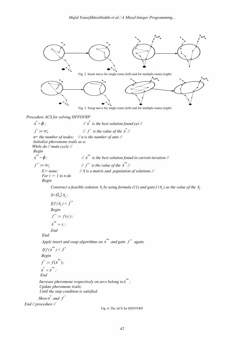
Fig. 2. Insert move for single route (left) and for multiple routes (right)

Fig. 3. Swap move for single route (left) and for multiple routes (right)

Procedure ACS for solving HFFOVRP

*s = ; // *s is the best solution found yet // * : ;f // *f is the value of the *s //

n= the number of nodes; // n is the number of ants // Initialize pheromone trails as u;

While do // main cycle // Begin

**s = ; // **s is the best solution found in current iteration // ** : ;f // **f is the value of the **s //

S:= none; // S is a matrix and population of solutions // For i := 1 to n do Begin

Construct a feasible solution is by using formula (11) and gain f ( is ) as the value of the is

S=S is ;

If f ( is ) < **f Begin

** : ( )i

f f s ; **

iss ;

End End; Apply insert and swap algorithms on **s and gain **f again.

If f ( **s ) < *f Begin

* **: ( )f f s ;

* **s s ;

End Increase pheromone respectively on arcs belong to **s ; Update pheromone trails;

Until the stop condition is satisfied.

Show *s and *f End // procedure //

Fig. 4. The ACS for HFFOVRP


42

4. Computational Results

In this section, our proposed meta-heuristic algorithm was tested on a set of HFFOVRP benchmark problems and compared to the solver Cplex 12.4 in AIMMS. AIMMS is an advanced development environment for building advanced planning systems and optimizing the problems in applied research studies. The ACS presented in Section 3, was coded in Matlab 7. All the experiments were implemented on a PC with Pentium 4 at 2.4GHZ and 2GB RAM running Windows XP Home Basic Operating system. Therefore, a new set consisting of eight tests numbered from 1 to 8 with sizes ranging from 11 to 50 nodes without the depot were derived from the well-known Taillard’s benchmark for Heterogeneous fleet Vehicle Routing Problem (HFFVRP). In this section, we first introduce the benchmark problems and then the detailed computational results obtained.

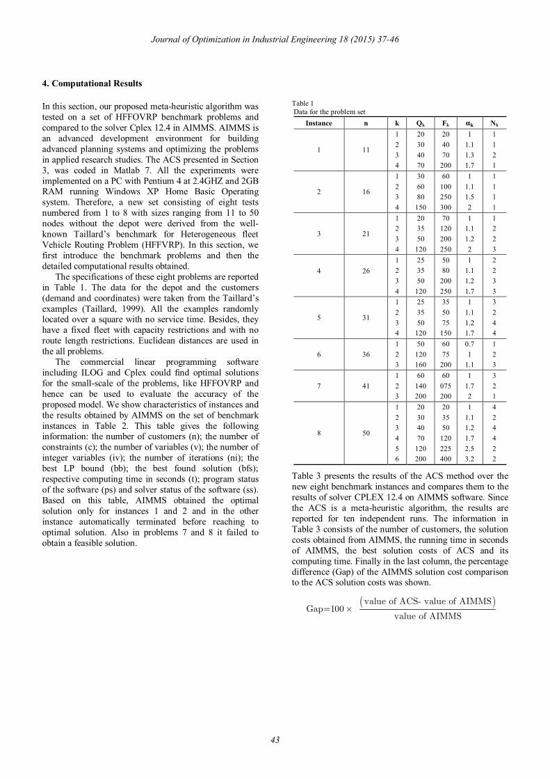
The specifications of these eight problems are reported in Table 1. The data for the depot and the customers (demand and coordinates) were taken from the Taillard’s examples (Taillard, 1999). All the examples randomly located over a square with no service time. Besides, they have a fixed fleet with capacity restrictions and with no route length restrictions. Euclidean distances are used in the all problems.

The commercial linear programming software including ILOG and Cplex could find optimal solutions for the small-scale of the problems, like HFFOVRP and hence can be used to evaluate the accuracy of the proposed model. We show characteristics of instances and the results obtained by AIMMS on the set of benchmark instances in Table 2. This table gives the following information: the number of customers (n); the number of constraints (c); the number of variables (v); the number of integer variables (iv); the number of iterations (ni); the best LP bound (bb); the best found solution (bfs); respective computing time in seconds (t); program status of the software (ps) and solver status of the software (ss). Based on this table, AIMMS obtained the optimal solution only for instances 1 and 2 and in the other instance automatically terminated before reaching to optimal solution. Also in problems 7 and 8 it failed to obtain a feasible solution.

Table 1 Data for the problem set

Instance n k Qk Fk 훂퐤 Nk

1 11

1 20 20 1 1 2 30 40 1.1 1 3 40 70 1.3 2 4 70 200 1.7 1

2 16

1 30 60 1 1 2 60 100 1.1 1 3 80 250 1.5 1 4 150 300 2 1

3 21

1 20 70 1 1 2 35 120 1.1 2 3 50 200 1.2 2 4 120 250 2 3

4

26

1 25 50 1 2 2 35 80 1.1 2 3 50 200 1.2 3 4 120 250 1.7 3

5 31

1 25 35 1 3 2 35 50 1.1 2 3 50 75 1.2 4 4 120 150 1.7 4

6 36 1 50 60 0.7 1 2 120 75 1 2 3 160 200 1.1 3

7 41 1 60 60 1 3 2 140 075 1.7 2 3 200 200 2 1

8 50

1 20 20 1 4 2 30 35 1.1 2 3 40 50 1.2 4 4 70 120 1.7 4 5 120 225 2.5 2 6 200 400 3.2 2

Table 3 presents the results of the ACS method over the new eight benchmark instances and compares them to the results of solver CPLEX 12.4 on AIMMS software. Since the ACS is a meta-heuristic algorithm, the results are reported for ten independent runs. The information in Table 3 consists of the number of customers, the solution costs obtained from AIMMS, the running time in seconds of AIMMS, the best solution costs of ACS and its computing time. Finally in the last column, the percentage difference (Gap) of the AIMMS solution cost comparison to the ACS solution costs was shown.

value of ACS- value of AIMMSGap=100

value of AIMMS


43

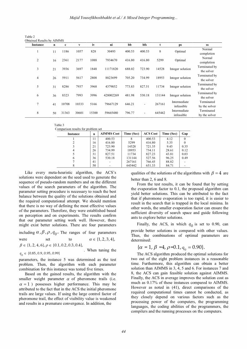
Table 2 Obtained Results by AIMMS

Instance n c v iv ni bb bfs t ps ss

1 11 1186 1057 828 30493 400.53 400.53 8 Optimal Normal

completion

2 16 2361 2177 1088 7934670 416.80 416.80 5299 Optimal Normal

completion

3 21 3936 3697 1848 11171820 688.02 723.90 14528 Integer solution Terminated by

the solver


the solver


the solver


the solver

7 41 10708 10333 5166 79667129 646.21 - 267161 Intermediate infeasible

Terminated by the solver

8 50 31363 30601 15300 59665480 796.77 - 645442 Intermediate

infeasible Terminated

by the solver

Table 3 Comparison results for problem set

Instance n AIMMS Cost Time (Sec) ACS Cost Time (Sec) Gap 1 11 400.53 8 400.53 4.12 0 2 16 416.80 5299 416.80 5.35 0 3 21 723.90 14528 721.35 9.45 0.35 4 26 734.99 18953 734.11 28.61 0.12 5 31 827.51 11734 827.23 43.81 0.03 6 36 530.18 131144 527.56 96.25 0.49 7 41 - 267161 766.45 88.82 - 8 50 - 645442 651.33 84.71 -

Like every meta-heuristic algorithm, the ACS’s solutions were dependent on the seed used to generate the sequence of pseudo-random numbers and on the different values of the search parameters of the algorithm. The parameter setting procedure is necessary to reach the best balance between the quality of the solutions obtained and the required computational attempt. We should mention that there is no way of defining the most effective values of the parameters. Therefore, they were established based on perception and on experiments. The results confirm that our parameter setting work well. However, there might exist better solutions. There are four parameters

including 0, , , .q The ranges of four parameters were set to {1, 2, 3, 4},

0 {0.85, 0.9, 0.95, 0.99}

{1, 2, 4, 6}, {0.1, 0.2 , 0.3, 0.4},

q. When tuning the

parameters, the instance 5 was determined as the test problem. Then, the algorithm with each parameter combination for this instance was tested five times.

Based on the gained results, the algorithm with the smaller weight parameter of pheromone trails (i.e.

1 ) possesses higher performance. This may be attributed to the fact that in the ACS the initial pheromone trails are large values. If using the large control factor of pheromone trail, the effect of visibility value is weakened and results in a premature convergence. In addition, the

qualities of the solutions of the algorithms with 4 are better than 2, 6 and 8.

From the test results, it can be found that by setting the evaporation factor to 0.1, the proposed algorithm can yield better solutions. This can be attributed to the fact that if pheromone evaporation is too rapid, it is easier to result in the search that is trapped in the local minima. In other words, the smaller evaporation factor can ensure the sufficient diversity of search space and guide following ants to explore better solutions.

Finally, the ACS, in which 0q is set to 0.90, can provide better solutions in compared with other values. Thus, the combinations of optimal parameters are determined:

0q{ = 1, =4, =0.1, 0.90}. The ACS algorithm produced the optimal solutions for

two out of the eight problem instances in a reasonable time. Furthermore, this algorithm can obtain a better solution than AIMMS in 3, 4, 5 and 6. For instances 7 and 8, the ACS can gain feasible solution against AIMMS. Finally, the ACS in average improves the solution cost as much as 0.17% of these instances compared to AIMMS. However as noted in (41), direct comparisons of the required computational times cannot be conducted, as they closely depend on various factors such as the processing power of the computers, the programming languages, the coding abilities of the programmers, the compilers and the running processes on the computers.


44

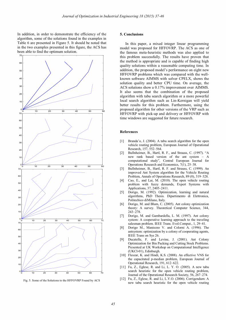
In addition, in order to demonstrate the efficiency of the algorithm, some of the solutions found in the examples in Table 6 are presented in Figure 5. It should be noted that in the two examples presented in this figure, the ACS has been able to find the optimum solution.

Fig. 5. Some of the Solutions to the HFFOVRP Found by ACS

5. Conclusions

In this paper, a mixed integer linear programming model was proposed for HFFOVRP. The ACS as one of the famous meta-heuristic methods was also applied to this problem successfully. The results have proven that the method is appropriate and is capable of finding high quality solutions within a reasonable computing time. In addition, the proposed model’s performance on eight new HFFOVRP problems which was compared with the well-known software AIMMS with solver CPELX, shows the solution quality and better CPU time. On average, the ACS solutions show a 0.17% improvement over AIMMS. It also seems that the combination of the proposed algorithm with tabu search algorithm or a more powerful local search algorithm such as Lin-Kernigan will yield better results for this problem. Furthermore, using the proposed algorithm for other versions of the VRP such as HFFOVRP with pick-up and delivery or HFFOVRP with time windows are suggested for future research.

References

[1] Brandaõ, J. (2004). A tabu search algorithm for the open vehicle routing problem, European Journal of Operational Research, 157, 552–564.

[2] Bullnheimer, B., Hartl, R. F., and Strauss, C. (1997). “A new rank based version of the ant system – A computational study”, Central European Journal for Operations Research and Economics, 7(1), 25–38.

[3] Bullnheimer, B., Hartl, R. F. and Strauss, C. (1999). An improved Ant System algorithm for the Vehicle Routing Problem, Annals of Operations Research, 89 (0), 319–328.

[4] Cao, E., and Lai, M. (2010). The open vehicle routing problem with fuzzy demands, Expert Systems with Applications, 37, 2405–2411.

[5] Dorigo, M. (1992). Optimization, learning and natural algorithms, PhD Thesis. Dipartimento di Elettronica, Politechico diMilano, Italy.

[6] Dorigo, M. and Blum, C. (2005). Ant colony optimization theory: A survey. Theoretical Computer Science, 344, 243–278.

[7] Dorigo, M. and Gambardella, L. M. (1997). Ant colony system: A cooperative learning approach to the traveling salesman problem. IEEE Trans. Evol.Comput., 1, 29–41.

[8] Dorigo M., Maniezzo V. and Colorni A. (1996). The antsystem: optimization by a colony of cooperating agents, IEEE Trans on Sys 26.

[9] Ducatelle, F. and Levine, J. (2001). Ant Colony Optimization for Bin Packing and Cutting Stock Problems. Presented at UK Workshop on Computational Intelligence (UKCI-01), Edinburgh.

[10] Fleszar, K. and Hindi, K.S. (2008). An effective VNS for the capacitated p-median problem, European Journal of Operational Research, 191, 612–622.

[11] Fu, Z., Eglese, R. and Li, L. Y. O. (2005). A new tabu search heuristic for the open vehicle routing problem, Journal of the Operational Research Society, 56, 267–274.

[12] Fu, Z., Eglese, R. and Li, L.Y.O. (2006). Corrigendum: A new tabu search heuristic for the open vehicle routing

0 10 20 30 40 50 600

10

20

30

40

50

60

70

0 10 20 30 40 50 600

10

20

30

40

50

60

70

0 10 20 30 40 50 60 700

10

20

30

40

50

60

70

0 10 20 30 40 50 60 700

10

20

30

40

50

60

70


45

problem, Journal of the Operational Research Society, 57, 1018.

[13] Geetha, S., Vanathi P. T. and Poonthalir, G. (2012). Metaheuristic approach for the multiple-depot vehicle routing problem, Applied Artificial Intelligence, 26(9), 878-901

[14] Letchford, A. N., Lysgaard, J. and Eglese, R. W. (2007). A branch-and-cut algorithm for the capacitated open vehicle routing problem, Journal of the Operational Research Society, 58, 1642–1651.

[15] Li, F., Golden, B. and Wasil, E. (2007). The open vehicle routing problem: Algorithms, large-scale test problems, and computational results, Computers and Operations Research, 34, 2918–2930.

[16] Li, X., Tian, P., and Aneja, Y. P. (2010). An adaptive memory programming metaheuristic for the heterogeneous fixed fleet vehicle routing problem, Transportation Research Part E, 46, 1111–1127.

[17] Maniezzo, V., Colorni, A. and Dorigo, M. (1994). The ant system applied to the quadratic assignment problem. Universite Libre de Bruxelles, Belgium, Tech. Rep. IRIDIA/94-28.

[18] McMellan, N., (2006). RNA Secondary Structure Prediction using Ant Colony Optimization, Master Thesis. School of Informatics, University of Edinburgh.

[19] MirHassani, S. A. and Abolghasemi N. (2011). A particle swarm optimization algorithm for open vehicle routing problem, Expert Systems with Applications, 38(9), 11547-11551.

[20] Ozfirat, P. M. and Ozkarahan, I. (2010). A Constraint programming heuristic for a heterogeneous vehicle routing problem with split deliveries, Applied Artificial Intelligence, 24(4), 277-294.

[21] Pisinger, D. and Ropke, S. (2007). A general heuristic for vehicle routing problems, Computers and Operations Research, 34, 2403–2435.

[22] Popovic, J. (1995). Vehicle routing in the case of uncertain demand: a Bayesian approach, Transportation Planning and Technology, 19(1), 19-29

[23] Reimann, M., Doerner, K. and Hartl, R. F. (2004). D-ants: savings based ants divide and conquer the vehicle routing problem, ComputersandOperations Research, 31, 563–591.

[24] Sariklis, D. and Powell, S. (2000). A heuristic method for the open vehicle routing problem, Journal of the Operational Research Society, 51, 564–573.

[25] Schrage, L. (1981). Formulation and structure of more complex/realistic routing and scheduling problems, Networks, 11, 229–232.

[26] Sedighpour, M., Ahmadi, V., Yousefikhoshbakht, M., Didehvar, F. and Rahmati, F. (2014). Solving the open vehicle routing problem by a hybrid ant colony optimization. Kuwait Journal of Science, 41 (3), 139-162.

[27] Syslo, M., Deo, N. and Kowalik, J. (1983). Discrete Optimization Algorithms with Pascal Programs, Prentice Hall.

[28] Taillard, E. D. (1999). A heuristic column generation method for the heterogeneous fleet VRP, RAIRO , 33, 1-14.

[29] Tarantilis, C. D., Ioannou, G., Kiranoudis, C.T. and Prastacos, G.P. (2005). Solving the open vehicle routing problem via a single parameter metaheuristic algorithm, Journal of the Operational Research Society, 56, 588–596.

[30] Tarantilis, C. D., Ioannou, G., Kiranoudis, C.T. and Prastacos, G.P. (2005). Solving the open vehicle routing

problem via a single parameter metaheuristic algorithm, Journal of the Operational Research Society, 56, 588–596.

[31] Teodorovic, D., Krcmar-Nozic, E. and Pavkovic, G. (1995). The mixed fleet stochastic vehicle routing problem, Transportation Planning and Technology, 19(1), 31-43

[32] Tzeng, G. H., Huang, W. C. and Teodorovic, D. (1997). A spatial and temporal bi‐criteria parallel‐savings‐based heuristic algorithm for solving vehicle routing problems with time windows, Transportation Planning and Technology, 20(2), 163-181

[33] Yousefi khoshbakht, M., Didehvar, F. and Rahmati, F. (2014). Solving the heterogeneous fixed fleet open vehicle routing problem by a combined metaheuristic algorithm. International Journal of Production Research, 52 (9), 2565-2575

[34] Yousefi khoshbakht, M., Didehvar, F. and Rahmati, F. (2014). A combination of modified tabu search and elite ant system to solve the vehicle routing problem with simultaneous pickup and delivery. Journal of Industrial and Production Engineering, 31 (2), 65-75

[35] Yousefi khoshbakht, M. and Khorram, E. (2012). Solving the vehicle routing problem by a hybrid meta-heuristic algorithm. Journal of Industrial Engineering International, 8 (1), 1-9

[36] Yousefi khoshbakht, M. and Sedighpour, M. (2012). A combination of sweep algorithm and elite ant colony optimization for solving the multiple traveling salesman problem. Proceedings of the Romanian Academy A, 13 (4), 295-302.


46

Documents

A Mixed Integer Programming Formulation for the ... · PDF fileA Mixed Integer Programming Formulation for the Heterogeneous Fixed Fleet Open Vehicle Routing Problem Majid Yousefikhoshbakhta,*,