Embed Size (px)
Citation preview
Course on Advanced Programming for
Scientific Computing
A Mixed Finite Element Solver forCoupled 3D/1D Fluid Problems
Prof. Luca Formaggia
A. Y. 2014-2015
Domenico Notaro 80443

Abstract
The main goal of this project is to develop of a general-purpose finite element solverfor large scale simulations of microcirculation.
Thanks to dimensional (or topological) model reduction techniques, the vessel treeis described as a one-dimensional (1D) manifold immersed in a three-dimensional(3D) interstitial volume. Vessels can be seen as concentrated sources to reduce thecomputational cost of simulations. However, concentrated sources lead to singularsolutions that still require computationally expensive graded meshes to guaranteeaccurate approximation. The main computational barrier consists in the ill-posedness ofrestriction operators (such as the trace operator) applied on manifolds with co-dimensionlarger than one. We overcome the computational challenges of approximating PDEs onmanifolds with high dimensionality gap by means of nonlocal restriction operators thatcombine standard traces with mean values of the solution on low dimensional manifolds.
This approach, originally developed by C. D’Angelo, is extended here to the mixedformulation of flow problems with applications to microcirculation. In this way weobtain a simultaneous approximation of velocity and pressure field that guaranteesgood accuracy with respect to mass conservation.
An outline of the remainder of the paper follows: Section 1 describe the generalmathematical framework of the coupled multiscale problem. The implementation of theabove model using the Finite Element library GetFEM++ is addressed in 2. We presentnumerical results from various benchmark problems to validate our solver. Finally,Section 3 contains a detailed description of the C++ code available at the followinglink:
https://github.com/domeniconotaro/PACS.
2

Contents
1 Mathematical Formulation 31.1 Coupling microcirculation with interstitial flow . . . . . . . . . . . . . . . . 41.2 Dimensional analysis . . . . . . . . . . . . . . . . . . . . . . . . . . . . . . . 61.3 Boundary conditions . . . . . . . . . . . . . . . . . . . . . . . . . . . . . . . 71.4 Compatibility conditions . . . . . . . . . . . . . . . . . . . . . . . . . . . . . 81.5 Weak formulation . . . . . . . . . . . . . . . . . . . . . . . . . . . . . . . . . 91.6 Numerical Approximation . . . . . . . . . . . . . . . . . . . . . . . . . . . . 10
2 GetFEM implementation 132.1 Uncoupled 3D and 1D problems . . . . . . . . . . . . . . . . . . . . . . . . . 13
2.1.1 Stand-alone tissue problem . . . . . . . . . . . . . . . . . . . . . . . 142.1.2 Stand-alone vessel network problem . . . . . . . . . . . . . . . . . . 15
2.2 Coupled 3D-1D problem with a single-branch network . . . . . . . . . . . . 182.3 Coupled 3D-1D problem with a single-bifurcation network . . . . . . . . . . 192.4 Code validation: primal vs mixed . . . . . . . . . . . . . . . . . . . . . . . . 21
3 C++ code 273.1 Re-design of the code . . . . . . . . . . . . . . . . . . . . . . . . . . . . . . . 273.2 Assembling improvements . . . . . . . . . . . . . . . . . . . . . . . . . . . . 313.3 The library problem3d1d . . . . . . . . . . . . . . . . . . . . . . . . . . . 363.4 Doxygen documentation . . . . . . . . . . . . . . . . . . . . . . . . . . . . . 37
1 Mathematical Formulation
We study a mathematical model for fluid transport in a permeable biological tissue perfusedby a vessel network with arbitrary topology. The domain in R3 where the model is definedis composed by two parts, Ωt and Ωv, denoting the interstitial volume and the vessel bedrespectively. Assuming that the vessels can be described as cylindrical tubes, we denotewith Γ the outer surface of Ωv while Λ indicates the 1D manifold representing the vesselcenterline [cfr. Fig.1]. The vessel radius R is generally subject to change in the network.
We consider the interstitial volume Ωt as an isotropic porous medium, described by theDarcy’s law. Ignoring inertial and body forces, it reads:
ut = − 1
µIK∇pt (1)
where ut is average filtration velocity vector in the tissue, IK is the permeability tensor, µis the viscosity of the fluid and pt is the fluid pressure. Recall that in the simple isotropic
3

Figure 1: On the left the interstitial tissue slab with one embedded capillary; on the rightreduction from 3D to 1D description of the capillary vessel.
case the permeability tensor is given by IK = k II, being k the scalar permeability and II theidentity tensor.
Concerning the vessels, we start assuming a steady incompressible Navier-Stokes modelfor blood flow, namely:
ρ (uv · ∇)uv − µ∆uv +∇pv = 0 (2)
where uv is the flow velocity, pv is the pressure and ρ the density of the fluid.
1.1 Coupling microcirculation with interstitial flow
At this stage the two problems are completely uncorrelated. Indeed, to close the problemwe need to impose continuity of the flow at the interface Γ = ∂Ωv ∪ ∂Ωt, namely:
uv · n = ut · n = Lp(pv − pt), uv · τττ = 0 on Γ , (3)
where n and τττ are the outward unit normal vector and unit tangent vector of the surface Γ,respectively, while Lp is the hydraulic conductivity of the vessel wall.
Finally, for the problem (1)-(5)-(3) to be uniquely solvable, in Section 1.3 we will specifysuitable boundary conditions on ∂Ωv and ∂Ωt.
Equations (1), (2), (3) identify a fully three-dimensional model able to capture thephenomena we are interested in. However, many technical difficulties arise in the numericalapproximation of the coupling between a complex network with the surrounding volume.To this purpose, we adopt the multiscale approach developed by C. D’Angelo1 to avoidresolving the complex 3D geometry of the network. We exploit the Immersed BoundaryMethod (IBM) combined with the assumption of large aspect ratio between vessel radiusand capillary axial length. This approach is represented in Figure 1. More precisely, weapply a suitable rescaling of the equations and let the capillary radius go to zero (R→ 0).
1 Multiscale Modelling of Metabolism and Transport Phenomena in Living Tissue, C. D’Angelo, 2007.
4

As a consequence, the three-dimensional description of the vessels is reduced to a simplifiedone-dimensional representation by replacing the immersed interface and the related interfaceconditions with an equivalent mass source, namely:
ut · n = f(pt, pv) on Γ , (4)
being f the flux per unit area released through the surface Γ: it is a point-wise constitutivelaw for the capillary leakage in terms of the fluid pressure.
Therefore, also at the modeling level a relevant simplification may be applied withoutsignificant loss of accuracy. In the case of microcirculation it is indeed possible to easilyderive a reduced flow model from the full Navier-Stokes equations: specifically, a quasi-static approximation is acceptable. To this purpose, we decompose the network Λ intoindividual branches Λi, i = 1, · · · , N . Branches are parametrized by the arc length si; atangent unit vector λλλi is also defined over each branch, accounting for an arbitrary branchorientation. Differentiation over the branches is defined using the tangent unit vector,namely ∂si := ∇ ·λλλi on Λi, i.e. ∂si represents the projection of ∇ along λi. The blood flowalong each branch of the network can be described by means of Poiseuille’s law for laminarstationary flow of incompressible viscous fluid through a cylindrical tube with radius R.According to Poiseuille’s flow, conservation of momentum and mass reads:
uv,i = −R2
8µ
∂pv,i∂si
λλλi and − πR2∂uv,i∂si
= gi on Λi , (5)
where gi is the transmural flux leaving the vessel. As a consequence of the geometricassumptions, the vessel velocity has fixed direction and unknown scalar component alongthe vessel, namely uv,i = uv,iλλλi. We shall hence formulate the vessel problem using thescalar unknown uv. The governing flow equations for the whole network Λ are obtained bysumming (5) over the index i.
Finally, the coupled problem for microcirculation and interstitial flow reads as follows:
µ
kut +∇pt = 0 in Ω
∇ · ut − f(pt, pv) δΛ = 0 in Ω
8µ
R2uv +
∂pv∂s
= 0 in Λ
∂uv∂s
+1
πR2f(pt, pv) = 0 in Λ
. (6)
Then, the constitutive law for the leakage of the vessel walls is provided by means of theStarling’s law of filtration,
f(pt, pv) = 2πRLp (pv − pt) , (7)
5

0
1
2
(uv0 , pv
0)
(uv1 , pv
1)
(uv2 , pv
2)
Figure 2: On the left, a simple network made by a single Y-shaped bifurcation. Arrowsshow the flow orientation: one inflow branch on the left of the bifurcation point, two outflowbranches on the right. On the right the related discretization of the vessel network: thedomain has been split into branches, the problem will be assembled over each branch andcompatibility conditions will be added at the junction point.
with
pt(s) =1
2πR
∫ 2π
0pt(s, θ) Rdθ . (8)
Since the vessel bed is approximated with its centerline, the average pv(s) coincides withits pointwise value pv(s).
Finally, we notice that in problem (6) the subregion Ωt has been identified with theentire domain Ω, because the one-dimensional manifold Λ has null measure in R3. Theabove notation will be extensively used in the remainder.
1.2 Dimensional analysis
To put into evidence the most significant mechanisms governing the flow between microcir-culation and the biological tissue, it is useful to write the equations in dimensionless form.First, we identify the characteristic dimensions of our problem: length, velocity and pressureare chosen as primary variables for the analysis. The corresponding characteristic valuesare: (i) the average spacing between capillary vessels d, (ii) the average velocity in thecapillary bed U , and (iii) the average pressure in the interstitial space P . Correspondingly,the dimensionless groups affecting our equations are:
- R′ =R
dnon-dimensional radius,
- κt =k
µ
P
Udhydraulic conductivity of the tissue,
6

- Q = 2πR′LpP
Uhydraulic conductivity of the capillary walls,
- κv =πR′4
8µ
Pd
Uhydraulic conductivity of the capillary bed.
Therefore, the coupled dimensionless problem of microcirculation and tissue interstitiumreads as follows:
1
κtut +∇pt = 0 in Ω
∇ · ut −Q (pv − pt) δΛ = 0 in Ω
πR′2
κvuv +
∂pv∂s
= 0 in Λ
∂uv∂s
+1
πR′2Q (pv − pt) = 0 in Λ
. (9)
For simplicity of notation, we used the same symbols for the dimensionless variables, i.evelocities and pressure scaled by U and P , respectively.
Remark 1. The code is entirely written in dimensionless form. As we will explain lateron in Sec. 3 the PDE coefficients can be easily set through an input list. For the sake ofcompleteness, we make the user able to set either the dimensionless parameters (R′, κt, Q, κv)or the dimensional ones (R, k, µ, Lp, d, P, U): in the latter case the adimensional analysis isperformed internally.
1.3 Boundary conditions
As mentioned previously, for the problem (9) to be well-posed we have to specify suitableboundary conditions (BCs) on both the tissue and vessel boundary, i.e. ∂Ω and ∂Λrespectively.
Since we aim to present the most generic setting, we assume the tissue interstitiumboundary to be partitioned as follows:
∂Ω = Γp ∪ Γu ,Γp ∩
Γu = ∅ . (10)
As suggested by the apices p and u, we enforce a given pressure distribution over Γp and/ora fixed value for the normal flux over Γu, namely:
pt = gt on Γp , (11)
ut · n = β( pt − p0 ) on Γu . (12)
In equation (12) p0 represents far field pressure value, while β can be interpreted as aneffective conductivity accounting for layers of tissue surrounding the considered sample.
7
Assuming that the interstitial pressure decays from pt to p0 over a distance comparable tothe sample characteristic size, D, dimensional analysis shows that a rough estimate of theconductivity is β = κt/D. For the pressure datum we require gt ∈ L2(Γp).
Concerning the network, we split the collection of extrema into two subsets: on boundaryextrema, Ep, we enforce a pressure distribution, on immersed extrema, Eu, we enforce theflux (hence the vessels velocity); namely:
pv = gv on Ep (13)
πR′2 uv = β( pv − p0 ) on Eu (14)
where gv is a boundary datum for which require measurability and square-summability,namely gv ∈ L2(Ep), while p0 and β are as above. In particular, in future applicationswe will always enforce a constant pressure drop P outv − P inv , that means we will adoptpiecewise-constant boundary data.
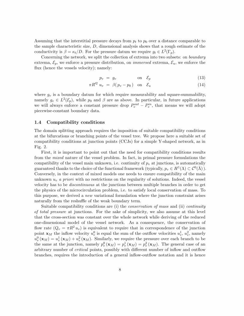
1.4 Compatibility conditions
The domain splitting approach requires the imposition of suitable compatibility conditionsat the bifurcations or branching points of the vessel tree. We propose here a suitable set ofcompatibility conditions at junction points (CCJs) for a simple Y-shaped network, as inFig. 2.
First, it is important to point out that the need for compatibility conditions resultsfrom the mixed nature of the vessel problem. In fact, in primal pressure formulations thecompatibility of the vessel main unknown, i.e. continuity of pv at junctions, is automaticallyguaranteed thanks to the choice of the functional framework (typically, pv ∈ H1(Λ) ⊂ C0(Λ) ).Conversely, in the context of mixed models one needs to ensure compatibility of the mainunknown uv a priori with no restrictions on the regularity of solutions. Indeed, the vesselvelocity has to be discontinuous at the junctions between multiple branches in order to getthe physics of the microcirculation problem, i.e. to satisfy local conservation of mass. Tothis purpose, we derived a new variational formulation where the junction constraint arisesnaturally from the reshuffle of the weak boundary term.
Suitable compatibility conditions are (i) the conservation of mass and (ii) continuityof total pressure at junctions. For the sake of simplicity, we also assume at this levelthat the cross-section was constant over the whole network while deriving of the reducedone-dimensional model of the vessel network. As a consequence, the conservation offlow rate (Qv = πR2 uv) is equivalent to require that in correspondence of the junctionpoint xM the inflow velocity u0
v is equal the sum of the outflow velocities u1v, u
2v, namely
u0v (xM ) = u1
v (xM ) + u2v (xM ). Similarly, we require the pressure over each branch to be
the same at the junction, namely p0v (xM ) = p1
v (xM ) = p2v (xM ). The general case of an
arbitrary number of critical points, possibly with different number of inflow and outflowbranches, requires the introduction of a general inflow-outflow notation and it is hence
8

postponed. Indeed, it is important to emphasize that such compatibility conditions areenforced in a natural way, at the level of the variational formulation.
1.5 Weak formulation
The derivation of a weak formulation of (9) that fulfils mass conservation is tricky andit is not reported in this paper. The idea is to integrate by parts the diverge terms insubequations (a) and (c) of (6) and then manipulate the resulting boundary term. In thisway we obtain, at the same time, a quasi-symmetric formulation of the coupled 3D/1Dproblem and the weak imposition of the mass conservation constraint. In particular, thefollowing integration by parts formula can be proved:∫
ΛπR′2
∂pv∂s
vv ds = −∫
ΛπR′2 pv
∂vv∂s
ds +[πR′2 pv vv
]Λout
Λin
+∑j ∈J
pv(sj)
∑i∈Pout
j
πR′2i vv |Λ+i−∑i∈Pin
j
πR′2i vv |Λ−i
,
(15)
where J indicates the set of junction points of the network, while P in/outj are the vesselswho enter/exit a given junction. The last term in (15) is indeed the weak counterpart of themass conservation constraint (written for the generic test function vv). See [?] for furtherdetails.
The variational formulation of problem (9) reads:Find ut ∈ Vt , pt ∈ Qt , uv ∈ Vv , pv ∈ Qv s.t.
( 1
κtut , vt
)Ω
+1
β
(ut · n , vt · n
)Γu−(pt , ∇ · vt
)Ω
=
= −(gt , vt · n
)Γp−(p0 , vt · n
)Γu
∀vt ∈ Vt(∇ · ut , qt
)Ω−(Q (pv − pt) , qt
)Λ
= 0 ∀qt ∈ Qt
( π2R′4
κvuv , vv
)Λ
+1
β[π2R′4 uv vv ]Eu −
(πR′2 pv , ∂svv
)Λ− 〈 vv, pv 〉J =
= −[πR′2 gv vv ]Ep − [πR′2 p0 vv ]Eu ∀vv ∈ Vv(πR′2 ∂suv , qv
)Λ
+(Q (pv − pt) , qv
)Λ
+ 〈uv, qv 〉J = 0 ∀qv ∈ Qv
(16)
We introduced the compact notation 〈 ·, · 〉J to indicate the junction term, that is the weakimposition of local mass conservation over each junction point in J , namely:
〈uv, qv 〉J := −∑j ∈J
∑i∈Pout
j
πR′2i uv |Λ+i−∑i∈Pin
j
πR′2i uv |Λ−i
qv(sj) . (17)
9

1.6 Numerical Approximation
The Finite Element Method is adopted to approximately solve (16). We denote with T ht anadmissible family of partitions of Ω into tetrahedrons K that satisfies the usual conditions ofa conforming triangulation of Ω. We use discontinuous piecewise-polynomial finite elementsfor pressure and Hdiv-conforming Raviart-Thomas for velocity, namely
Ykh :=wh ∈ L2 (Ω) : wh|K ∈ Pk−1(K) ∀K ∈ T ht
, (18)
RTkh :=wh ∈ H(div,Ω) : wh|K ∈ Pk−1(K; Rd)⊕ xPk−1(K) ∀K ∈ T ht
, (19)
for every integer k ≥ 0, where Pk indicates the standard space of polynomials of degree≤ k in the variables x = (x1, . . . , xd). For the simulations presented later on, the lowestorder Raviart-Thomas approximation has been adopted, corresponding to k = 0 above.
Concerning the capillary network, we split the discrete domain into segments, Λh =⋃Ni=1 Λhi , being where Λhi is a finite element mesh on the one-dimensional manifold Λi. The
solution of (16)(c),(d) over a given branch Λi is approximated using continuous piecewise-polynomial finite element spaces for both pressure and velocity. Since we want the vesselvelocity to be discontinuous at multiple junctions [cfr. Section 1.4], we define the relatedfinite element space over the whole network as the collection of the local spaces of the singlebranches. We have the following trial spaces for vessel pressure and velocity, respectively:
Xk+1h (Λ) :=
wh ∈ C0(Λ) : wh|S ∈ Pk+1 (S) ∀S ∈ Λh
, (20)
Wk+2h (Λ) :=
N⋃i=1
Xk+2h (Λi) , (21)
for every integer k ≥ 0. As a result, we use generalized Taylor-Hood elements on eachnetwork branch, satisfying in this way the local stability of the mixed finite element pair forthe network. At the same time, we guarantee that the pressure approximation is continuousover the entire network Λ. In particular, for the numerical experiments shown later on wehave used the lowest order, that is k = 0.
We can now derive a discrete formulation of our problem by projecting the continuousinfinite-dimensional PDEs over the discrete spaces defined above. Then, by writing thediscrete unknowns as linear combinations of the finite element base functions, we can deducethe following linear system:
Mtt −DTtt O O
Dtt Btt O −BtvO O Mvv −DT
vv − JTvvO −Bvt Dvv + Jvv Bvv
Ut
Pt
Uv
Pv
=
Ft
0
Fv
0
. (22)
10
Submatrices and subvectors are defined as follows:
[Mtt]i,j :=( 1
κtϕϕϕjt , ϕϕϕ
it
)Ω
+1
β
(ϕϕϕjt · n , ϕϕϕit · n
)Γu
Mtt ∈ RNht ×Nh
t ,
[Dtt]i,j :=(∇ ·ϕϕϕjt , ψit
)Ω
Dtt ∈ RNht ×Mh
t ,
[Btt]i,j :=(Qψjt δΛh
, ψit)
ΩBtt ∈ RM
ht ×Mh
t ,
[Btv]i,j :=(Qψjv δΛh
, ψit)
ΩBtv ∈ RM
ht ×Mh
v ,
[Bvt]i,j :=(Qψjt , ψ
iv
)Λ
Bvt ∈ RMhv×Mh
t ,
[Bvv]i,j :=(Qψjv , ψ
iv
)Λ
Mtt ∈ RMhv×Mh
v ,
[Mvv]i,j :=( π2R′4
κvϕjv , ϕ
iv
)Λ
+1
β[π2R′4 ϕjv ϕ
iv ]Eu Mvv ∈ RN
hv×Nh
v ,
[Dvv]i,j :=(πR′2 ∂sϕ
jv , ψ
iv
)Λ
Dvv ∈ RNhv×Mh
v ,
[Jvv]i,j := 〈 [ϕjv], ψiv 〉J Jvv ∈ RNhv×Mh
v ,
[Ft]i := −(ght , ϕϕϕ
it · n
)Γp−(ph0 , ϕϕϕ
it · n
)Γu
Ft ∈ RNht ,
[Fv]i := −[πR′2 gv ϕiv ] Ep − [πR′2 p0 ϕ
iv ] Eu Fv ∈ RN
hv ,
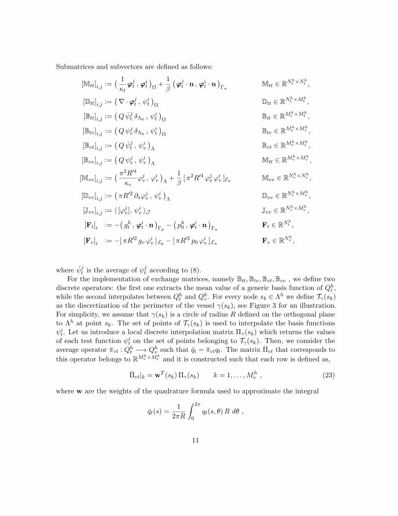
where ψjt is the average of ψjt according to (8).For the implementation of exchange matrices, namely Btt,Btv,Bvt,Bvv , we define two
discrete operators: the first one extracts the mean value of a generic basis function of Qht ,while the second interpolates between Qht and Qhv . For every node sk ∈ Λh we define Tγ(sk)as the discretization of the perimeter of the vessel γ(sk), see Figure 3 for an illustration.For simplicity, we assume that γ(sk) is a circle of radius R defined on the orthogonal planeto Λh at point sk. The set of points of Tγ(sk) is used to interpolate the basis functionsψit. Let us introduce a local discrete interpolation matrix Πγ(sk) which returns the valuesof each test function ψit on the set of points belonging to Tγ(sk). Then, we consider theaverage operator πvt : Qht −→ Qhv such that qt = πvtqt. The matrix Πvt that corresponds to
this operator belongs to RMhv×Mh
t and it is constructed such that each row is defined as,
Πvt|k = wT (sk) Πγ(sk) k = 1, . . . ,Mhv , (23)
where w are the weights of the quadrature formula used to approximate the integral
qt(s) =1
2πR
∫ 2π
0qt(s, θ)R dθ ,
11

γ(sk)
Λhsk
Tγ(sk)
Figure 3: Illustration of the vessel with its centerline Λh, a cross section, its perimeter γ(sk)and its discretization Tγ(sk) used for the definition of the interface operators πvt : Qht −→ Qhvand πtv : Qhv −→ Qht .
on the nodes belonging to Tγ(sk). The discrete interpolation operator πtv : Qhv −→ Qhtreturns the value of each basis function belonging to Qht in correspondence of nodes of Qhv .
In algebraic form it is expressed as an interpolation matrix Πtv ∈ RMhv×Mh
t . Using thesetools we obtain:
Btt = ΠTvtMP
vv Πvt , (24)
Btv = ΠTvtMP
vv , (25)
Bvt = MPvv Πvt , (26)
Bvv = MPvv , (27)
being MPvv the pressure mass matrix for the vessel problem defined by[
MPvv
]i,j
:=(Qψjv , ψ
iv
)Λ.
Concerning the implementation of junction compatibility conditions, we introduce alinear operator giving the restriction with sign of a basis function of V h
v over a given junctionnode. For a given k ∈ J , we define Rk : V h
v −→ R such that:
Rk(ϕjv ) :=
+πR′2l ϕ
jv(sk) j in Λhl ∧ l ∈ Poutk
−πR′2l ϕjv(sk) j in Λhl ∧ l ∈ P ink
, (28)
for all j = 1, . . . , Nhv , where the expression ”j in Λh
l ” means that the j-th dof is linkedto some vertex of the l-th branch. Note that we are implicitly using the usual propertyof Lagrangian finite element basis functions, i.e. that they vanish on all nodes except the
12
related one. As a consequence, our definition is consistent for all junction vertexes. Indeed,Rk may only assume values
−πR′2l , 0,+πR′2l
for some l and in particular Rk(ϕjv ) = 0
for all couples of indexes (k, j) that are uncorrelated. Furthermore, the definition of Rk canbe trivially extended to all network vertexes. Using this operator, the generic (i, j) elementof Jvv may be computed as follows:
[Jvv]i,j = −∑k∈J
Rk(ϕjv ) ψiv(sk) . (29)
2 GetFEM implementation
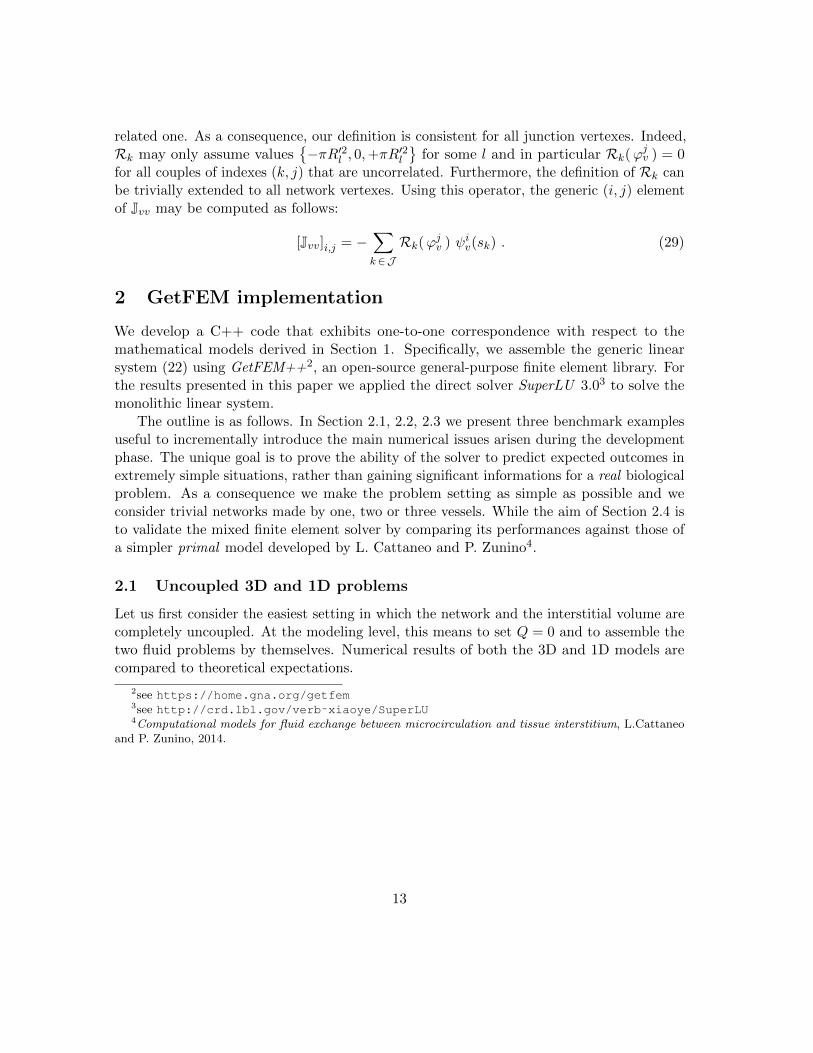
We develop a C++ code that exhibits one-to-one correspondence with respect to themathematical models derived in Section 1. Specifically, we assemble the generic linearsystem (22) using GetFEM++2, an open-source general-purpose finite element library. Forthe results presented in this paper we applied the direct solver SuperLU 3.03 to solve themonolithic linear system.
The outline is as follows. In Section 2.1, 2.2, 2.3 we present three benchmark examplesuseful to incrementally introduce the main numerical issues arisen during the developmentphase. The unique goal is to prove the ability of the solver to predict expected outcomes inextremely simple situations, rather than gaining significant informations for a real biologicalproblem. As a consequence we make the problem setting as simple as possible and weconsider trivial networks made by one, two or three vessels. While the aim of Section 2.4 isto validate the mixed finite element solver by comparing its performances against those ofa simpler primal model developed by L. Cattaneo and P. Zunino4.
2.1 Uncoupled 3D and 1D problems
Let us first consider the easiest setting in which the network and the interstitial volume arecompletely uncoupled. At the modeling level, this means to set Q = 0 and to assemble thetwo fluid problems by themselves. Numerical results of both the 3D and 1D models arecompared to theoretical expectations.
2see https://home.gna.org/getfem3see http://crd.lbl.gov/verb˜xiaoye/SuperLU4Computational models for fluid exchange between microcirculation and tissue interstitium, L.Cattaneo
and P. Zunino, 2014.
13

2.1.1 Stand-alone tissue problem
The mixed formulation of the three-dimensional Darcy’s problem in the interstitial volumeΩ ⊂ Rd reads:
1
κtut +∇pt = 0 in Ω
∇ · ut = ft in Ω
, (30)
where ft ∈ L2 (Ω) represents an arbitrary mass source term distributed over the tissuevolume. We notice that in the case of coupled (Q 6= 0) problems it turns into a localterm concentrated over the network Λ [cfr. (7)]. Problem (30) is complemented withhomogeneous conditions at the outer faces of the tissue slab, namely:
gt = 0 on ∂Ω . (31)
We adopt our mixed solver to approximate solve the linear system associated to (30), thatlooks similar to the top-left block of (22):[
Mtt −DTtt
Dtt O
][Ut
Pt
]=
[0
Gt
]. (32)
In particular, we consider a very simple setting where the exact solution is known. Let usconsider a simple fictional domain corresponding to a unitary cube in R3, namely Ω = [ 0, 1 ]3.The tissue sample is discretized using a tetrahedral structured mesh with characteristic sizeh = 1/20, as shown in Fig. 4. It is easy to check that an admissible solution of Darcy’sproblem (30) on a three-dimensional parallelepiped Ω = [ 0, Lx ]× [ 0, Ly ]× [ 0, Lz ] is givenby the following sinusoid:
pext = sin
(2π x
Lx
)sin
(2π y
Ly
)sin
(2π z
Lz
), (33)
who evidently fulfils the boundary condition (31). The related velocity field follows fromDarcy’s law (30)(a):
uext = −κt∇pext = −2πκt
1/Lx cos
(2π x
Lx
)sin
(2π y
Ly
)sin
(2π z
Lz
)1/Ly sin
(2π x
Lx
)cos
(2π y
Ly
)sin
(2π z
Lz
)1/Lz sin
(2π x
Lx
)sin
(2π y
Ly
)cos
(2π z
Lz
)
. (34)
Finally, we substitute the expression (34) into the mass equation (30)(b) to obtain thedatum:
gt = ∇ · uext = 4π2κt
(1
L2x
+1
L2y
+1
L2z
)pext . (35)
14

Figure 4: On the left, the discretization of the single-branch network: it is made by 21equally distributed nodes, Λh =
⋃20j=1 [ sj−1, sj ]. On the right the triangulation of the tissue
domain Ωh. In both cases we chose h = 0.05.
We specify the mass source (35) in the solver and compute the numerical solution (pht ,uht ).
As shown in Figure 2.1.1 there is full compliance between the computed solution and expectedone (33),(34). In particular, the interstitial pressure’s values belong to the expected interval,[−1, 1 ], while the magnitude of the computed velocity assumes values in [ 0, 2π ].
Remark 2. Pk projection of the discrete Raviart-Thomas velocityAs far as we know there are still many technical issues in dealing with non-lagrangian finiteelements in GetFEM++. In particular, there is no automatic way to interpolate on thespace RT0 nor to export a function belonging to this space for post-processing. To overcomethis issue we introduce the orthogonal L2-projection on the space of piecewise polynomialsPk, namely Πk
0,Ω : H (div,Ω) −→ [Pk (Ω) ]d. In the whole post-processing phase we use
Πk0,Ωu
ht as surrogate of the Hdiv-conforming Raviart-Thomas approximation uht . In fact
the former lives in standard lagrangian finite element spaces and we can apply the routinesprovided by the GetFEM library.
2.1.2 Stand-alone vessel network problem
The one-dimensional Poiseuille’s problem of fluid flow within the microcirculatory networkin its mixed formulation is given by
πR′2
κvuv +
∂pv∂s
= 0 s ∈ Λ
∂uv∂s
= 0 s ∈ Λ
. (36)
15

Figure 5: Numerical solution of (30) with unitary parameters Lx = Ly = Lz = 1, κt = 1.On the left the interstitial pressure pht , on the right the magnitude of the velocity field |uht |.
We enforce non-homogeneous fully-pressure boundary conditions at the extrema of thenetwork, namely:
gv(0) = 1 and gv(1) = 0 . (37)
The discretization of problem (36) turns into the resolution of a linear system equivalent tothebottom-right block of (22), namely:[
Mvv −DTvv
Dvv O
][Uv
Pv
]=
[Fv
0
]. (38)
We aim to solve the linear system (38) for an extremely simple vessel network made by asingle unitary vessel, Λ = [ 0, 1 ]. The 1D domain is discretized using 21 equally distributednodes [see Fig. 4(b) ]. The exact solution for such a simplified case can be derived by hand,namely:
pexv (s) = 1− s
2, (39)
uexv (s) = − κvπ R′2
∂pv∂s≡ κv
2πR′2. (40)
Theoretical expectations are fully confirmed from numerical results, as shown in Figure 6.As expected the pressure is linearly decreasing between the imposed boundary values 1 and0, while velocity is constant and equal to its expected value 1/2π. As a consequence, weassert that our solver behaves properly at least for what concerns the assembling of vesselterms.
16

arc lenght s
0 0.1 0.2 0.3 0.4 0.5 0.6 0.7 0.8 0.9 1
pressure pv
0.5
0.75
1
pv(s) = 1-s/2
ph
v(s) : h=0.2
ph
v(s) : h=0.1
ph
v(s) : h=0.05
arc lenght s
0 0.1 0.2 0.3 0.4 0.5 0.6 0.7 0.8 0.9 1
velocity uv
0
0.05
0.1
0.15
0.2
0.25
0.3
uv(s) = 1/2π
uh
v(s) : h=0.2
uh
v(s) : h=0.1
uh
v(s) : h=0.05
Figure 6: Numerical solution of (38) with unitary parameters R′ = 1, κv = 1. On the topthe 3D visualization (-Z view). On the bottom the 1D visualization of capillary pressure andvelocity as functions of the arc length s: the exact solution trend is compared to numericalvalues with 5, 10, 20 elements respectively. Boundary conditions are not exactly fulfilledbecause we used the lowest order approximation P0/P1, hence a centred approximation forpressure. To overcome this issue we shall use Pk/Pk+1 FE approximations with k > 0 [cfr.Fig. ?? ]. If this is the case the integration over a generic discrete capillary with more thanone vertex would be exact.
17

Figure 7: Computational domain for test-case II. The discrete network Λh is made bya single vessel immersed in a unitary slab of tissue interstitium, Ωh. We have used adiscretization step h = 0.05 for both the 1D and 3D problems.
2.2 Coupled 3D-1D problem with a single-branch network
To keep away any suspiciousness about the implementation of the coupling term betweenvessel network and the porous medium, we considered the case of a straight vessel immersedin a unitary cube of interstitial tissue [see Fig. 7 ]. For such a simple setting, we caneasily isolate the exchange terms. The coupled differential problem is given by (9). At themodeling level, the only significant simplification of the present test-case is that we don’thave to deal with compatibility conditions at bifurcations of the vessel tree. Therefore, byrepeating the argument of section 1, we obtain a linear system that is the specializationof (22) for Jvv = O. The mixed finite element solver is used to approximately solve themonolithic system. We adopt the unitary geometries presented in the first test-case. Sincewe have no analytical solution in this case, we exploit the numerical solution proposed by J.Chapman and R. Shipley5 for the single branch problem. In that work the authors model afluid flow through the leaky neovasculature and porous interstitium of a solid tumor, inparticular they consider the simplest case of an isolated capillary immersed in a tumortissue, giving rise to the the same problem addressed here. Then, in order to reproducenumerical results of [?] we choose the non-dimensional parameters of the problem as follows:
R′ = 10−2 , κt = 4 , κv = π R′3/8Lp , Q = 2π (41)
5Multiscale modelling of fluid and drug transport in vascular tumours., J. Chapman and R. Shipley, 2010
18

s
0 0.1 0.2 0.3 0.4 0.5 0.6 0.7 0.8 0.9 1
pv(s)
0
0.1
0.2
0.3
0.4
0.5
0.6
0.7
0.8
0.9
1
Lp=10
-4
Lp=2x10
-6
Lp=10
-6
Lp=5x10
-7
Lp=10
-7
Lp=10
-8
Figure 8: Numerical solution of the Chapman benchmark problem obtained with h = 0.05and dimensionless parameters R′ = 10−2, κt = 4, κv = π R′3/8Lp, Q = 2π. We report thevessel pressure as function of arclength phv(s) for different vascular permeabilities Lp =10−4, 2× 10⁻⁶, 10−6, 5× 10⁻⁷, 10−7, 10−8. To be compared with Fig.7 in [Chapman2008].
where Lp ∈
10−4, 2× 10⁻⁶, 10−6, 5× 10⁻⁷, 10−7, 10−8
is an array of non-dimensionalvascular permeability. The boundary datum in this case is given by:
gv(0) = 1.0 and gv(1) = 0.5 . (42)
In Figure 8 we represent the capillary pressure as a function of arc-length for differentvascular permeabilities. We can observe perfect agreement with the the plots shown in[?] (not reported here). Moreover, we notice that for the lowest value of the vascularpermeability Lp, corresponding to an almost impermeable vessel, the computational modelpredicts a linearly decreasing pressure, in agreement with the Poiseuille equation thatgoverns the flow. Conversely, for high permeability values there is a substantial deviationfrom the linear trend because the leakage dominates over the axial flow component.
2.3 Coupled 3D-1D problem with a single-bifurcation network
With the third and final step of the code verification phase we face the fundamental issueof mass conservation at the discrete level. For this purpose, we adopt a vessels networkslightly more complicated than the previous one, in which a single junction point is present[see Fig. 9 ]. For simplicity, we assume the average radius to be constant over the three
19

Figure 9: Computational domain for test-case III. The discrete vessels network Λh is madeby three capillaries affecting the same junction point xM = (0.5, 0.5, 0.5): Λ0
h enteringbranch, Λ1
h and Λ2h exiting branches. The tissue interstitium domain Ωh is a unit cube, as
in test cases I and II. We have used a discretization step h = 0.05 for both the 1D and 3Dproblems.
20

vessels [cfr. 1.4]. We observe that the conservation of total pressure,
p0v(xM ) = p1
v(xM ) = p2v(xM ) ≡ pv(xM ) , (43)
is automatically ensured thanks to the use of continuous finite elements for the vesselspressure approximation. Conversely, in order to impose the mass conservation constraint,
u0v(xM ) = u1
v(xM ) + u2v(xM ) , (44)
we have to implement the compatibility condition. In practice, in the simple Y-shapedconfiguration, we first identify the FEM degrees of freedom (dof) related to the samejunction node. For those dof we add in some specific entries of the problem matrix +1 foreach inflow branch and −1 for each outflow branch. This observation allows us to bypassthe non-trivial issue of assembling the compatibility matrix Jvv for a generic network withmultiple junctions [cfr. (29) ]. Since this is a practical rather than theoretical issue, weprefer to postpone its discussion to Section 3.
Using our computational model we assemble the linear system (22) on the computationaldomain (Ωh,Λh) described in Fig. 9. Boundary conditions are as in the previous example.We notice that both vessels pressure and velocity [cfr. top panel] confirm the expectedbehaviour along the network: the former is continuous everywhere and it correctly decreasesbetween the inlet and the outlet values; the latter is almost constant over each branch andit halves after the junction. We conclude that conditions (43) and (44) are fulfilled alsoat the numerical level. Furthermore, Fig.10(bottom) confirms that, also in this case, the3D/1D coupling behaves correctly.
2.4 Code validation: primal vs mixed
We aim to validate our computational model in its ultimate version. For this purpose,we shall face a more complex problem where we put together the ingredients introducedthrough the above test-cases. Once the validation is achieved, we shall apply our tool insome real life circumstances.
The primal or pressure formulation of the microcirculation problem reads
−κt ∆pt −Q (pv − pt) δΛ = 0 in Ω
ut = −κt∇pt in Ω
−κv∂2pv∂s2
+Q (pv − pt) = 0 in Λ
uv = − κvπR′2
∂pv∂s
λλλ in Λ
(45)
The two velocity fields, ut and uv, may be easily computed a posteriori once one knowsthe pressures. By repeating the procedure seen in Sections ??, ??, 1.6 one can derive the
21

Figure 10: Numerical solutions of the coupled 3D/1D fluid problem obtained with h = 0.05and unitary dimensionless parameters κt = 1, κv = 1, Q = 1, R′ = 1. (top) Vessels solution(phv , u
hv) at the longitudinal medium plane. (bottom) Evaluation of the coupling between
3D and 1D pressures and velocities.
22

Figure 11: Computational domain for the validation experiment. The network Λh is madeby 46 segments for a total length of 15.0 and an average radius R′ = 0.05; it is immersedin a unit cube of tissue interstitium Ωh = [ 0, 1 ]3. Black segments represent dead-endcapillaries.
following algebraic formulation:[Att + Btt Btv
Bvt Avv + Bvv
][Pt
Pv
]=
[Ft
Fv
](46)
where Att, Avv are the stiffness matrices for tissue and vessels problems respectively, namely:
[Att]i,j := κt(∇ψjt , ∇ψit
)Ω
[Avv]i,j := κv(∂sψ
jv , ∂sψ
iv
)Λ
.
The exchange matrices Btt,Btv,Bvt,Bvv, as well as the right hand sides are defined as inSection 1.6. By comparing (??) with (22) it is clear that the primal problem is easier toassemble and to solve w.r.t. the mixed one. With the resolution of both pressure andvelocity, we aim to gain the advantage of a more accurate approximation, mainly in termsof satisfaction of the mass conservation’s constraint.
We consider the coupled domain (Ω,Λ) in Fig. ?? consisting of a non trivial one-dimensional manifold immersed in a three-dimensional unitary cube. The average radius ofthe capillary vessels is assumed to be constant and set to R = 5 µm. The characteristiclength of the problem is chosen as the dimension of the tissue slab, d = 100 µm. Avascularized healthy tissue is characterized by an average interstitial pressure P = 1 mmHg
23

PRIMAL DUAL
dof number [ ] 3×10³ 1.5×10⁵
CPU time [ s ] 2.51 453.8
cond number [ ] 2×10⁵ 7×10⁴
Table 1: Characterization of the SuperLU solving algorithm.
and by a characteristic flow speed in the capillary bed of U = 100 µm/s. The parametersthat characterize the transport properties of the tissue are the hydraulic conductivity of theinterstitium, k = 10−18 m2, the hydraulic conductivity of the capillary walls, Lp = 10−12
m2 s/kg and the plasma viscosity µ = 4× 10⁻³ kg/m s. Given these data, we compute thedimensionless groups defined in Section 1.2:
R′ = 0.05, κt = 3.33× 10⁻⁶, Q = 4.19× 10⁻⁷, κv = 8.18× 10⁻² . (47)
Since κv, the dimensionless conductivity of the capillary bed, is significantly larger thanthe other transport quantities, we infer that, as expected, the transport in the coupledcapillary/interstitial medium is dominated by the flow in the vascular network.
We apply both the mixed and primal solver with 48000 four-nodes tetrahedral elementsfor the tissue slab Ωh and 1410 linear elements for the discrete network Λh. For the 1Dvessels network problem we adopt standard continuous piecewise-linear finite elements forpressure while non-standard local piecewise-quadratic finite elements have been implementedto approximate the velocity at each branch. Regarding the 3D tissue interstitium problem,we adopt discontinuous piecewise-constant finite element for pressure and H(div)-conforminglow order Raviart-Thomas finite element for velocity. Solving times and condition numberare reported in Tab. 2.4. As expected, the primal code is very much faster than the mixedone who has to solve a monolithic system that is 15 times greater. Figures 12-13 showresults of the simulations. It is clear from the visual comparison [cfr. Fig. 13] that theaccuracy of the mixed approximation of 3D velocity field is significantly better than theprimal approximation. Of course, we pay a worse accuracy for the 3D pressure. Concerningthe vessels network problem we omit the comparative view since no substantial differencewould be appreciated.
24

Figure 12: Numerical solution of the 1D vessel problem, (pv,h, uv,h) obtained with h = 0.05and non-dimensional parameters R′ = 0.05, Q = 4.189× 10⁻⁷, κv = 0.082. As expected thepressure (left) is almost linearly decreasing between the imposed boundary values 2 and 1and it is continuous at junctions while velocity (right) is almost constant over each branchand it correctly splits at junctions. We used a mixed P1/P2 finite element approximationfor capillary pressure and velocity, respectively. We decide to do not report the outcomeof primal code since there would be no difference to the eye [cfr. Tab. ??]. Note that, inagreement with Sec. ?? uv,h is null (dark blue) over the three dead-ends.
25
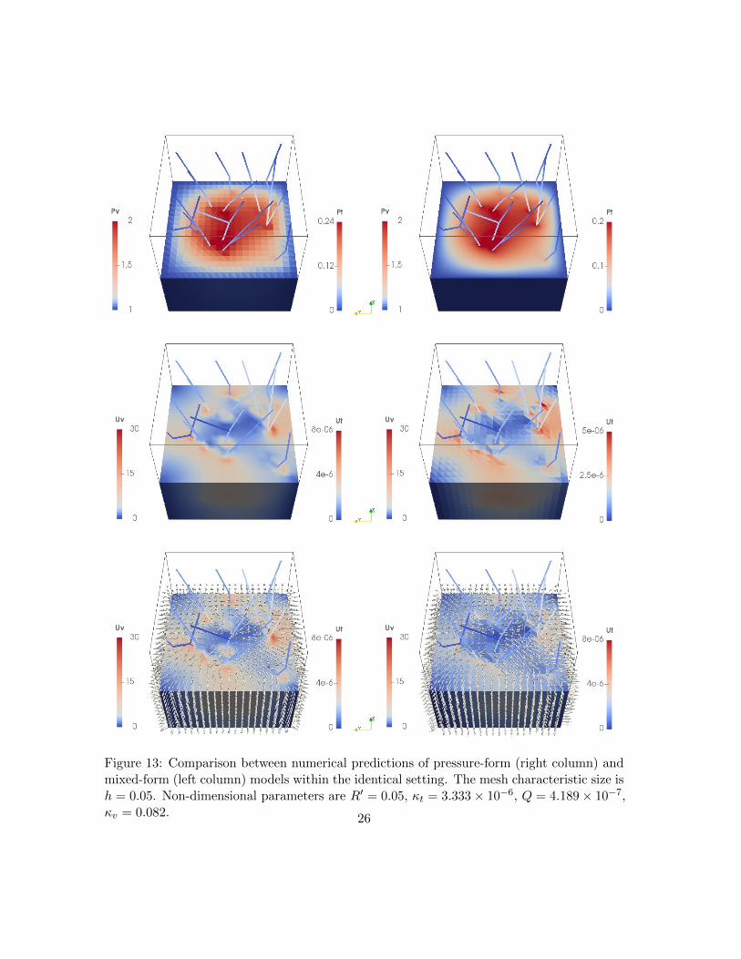
Figure 13: Comparison between numerical predictions of pressure-form (right column) andmixed-form (left column) models within the identical setting. The mesh characteristic size ish = 0.05. Non-dimensional parameters are R′ = 0.05, κt = 3.333× 10⁻⁶, Q = 4.189× 10⁻⁷,κv = 0.082. 26

3 C++ code
The latest stable release of the code is available at the following link:
https://github.com/domeniconotaro/PACS.
Let us briefly review the main achievements. The starting point is the code developed byL. Cattaneo for the tumor growth problem, available in src/4 primalmixed/primal.This is a first attempt to implement a finite element solver for coupled problems withdimensionality gap. However, it presents three main lacks: (i) it has no structure, the wholeproject has been implemented in one unreadable file main.cc, (ii) many functionalities arehard-coded and (iii) it does not conserve mass. Therefore, we improved and extended theavailable code in order to account for new purposes and applications. First, we re-designedthe whole code in a more harmonic and C++11 oriented way; then, we improved theimplementation of both tissue and vessel problems to gain the advantages of a mixedpressure-velocity formulation. At the end, the survivor of the primal code within the presentpackage are limited to a few lines.
3.1 Re-design of the code
Before starting with significant modifications and improvements, we decided to re-organizethe available code in such a way that the new C++11 standard is adopted.
First, in order to make the code more readable, we unified the terminology and make itconsistent with that of the numerical model we derived in the first section of this contribution.This is meant to facilitate future users and developers who are now guarantee about theone-to-one correspondence between theory and implementation.
Then, as first real modification, we export the declaration of the main structure rep-resenting the 3D/1D problem to an appropriate header file (problem3d1d.hpp). Asa well-known practise in C++ programming, the definition of the class has been movedto a source file (problem3d1d.cpp). We keep inside the main class all the attributeswho effectively identify an instance of the problem, such as the meshes, finite elementmethods, boundary conditions and so on. On the other hand, external attributes such asthe user-defined descriptors of the algorithm (descr3d1d.hpp), the dimensions of theproblem (dof3d1d.hpp) or physical parameters (param3d1d.hpp) have been moved toproper header files.
Furthermore, following the two main design principles of OOP, namely encapsulationand information hiding, we completely re-organize members’ scope. In this way, we define asimple interface between the computational model and users: the whole internal structurehas private scope while public accessors are eventually provided to inspect the attributes.
27

//! Main class defining the coupled 3D/1D fluid problem.class problem3d1d
public:
//! Constructor/*!
It links integration methods and finite element methods to themeshes
*/problem3d1d(void) :
mimt(mesht), mimv(meshv),mf_Pt(mesht), mf_coeft(mesht), mf_Ut(mesht),mf_Pv(meshv), mf_coefv(meshv)
//! Initialize the problem/*!
1. Read the .param filename from standard input2. Import problem descriptors (file paths, GetFEM types, ...)3. Import mesh for tissue (3D) and vessel network (1D)4. Set finite elements and integration methods5. Build problem parameters6. Build the list of tissue boundary data7. Build the list of vessel boundary (and junction) data
*/void init (int argc, char *argv[]);//! Assemble the problem/*!
1. Initialize problem matrices and vectors2. Build the monolithic matrix AM3. Build the monolithic rhs FM
*/void assembly (void);//! Solve the problem/*!
Solve the monolithic system AM*UM=FM (direct or iterative)
*/bool solve (void);//! Export results into vtk files/*!
Export solutions Ut, Pt, Uv, Pv from the monolithic array UM
*/void export_vtk (const string & suff = "");//! Compute mean tissue pressureinline scalar_type mean_pt (void)
28

return asm_mean(mf_Pt, mimt,gmm::sub_vector(UM, gmm::sub_interval(dof.Ut(), dof.Pt())));
//! Compute mean vessel pressureinline scalar_type mean_pv (void)
return asm_mean(mf_Pv, mimv,gmm::sub_vector(UM,
gmm::sub_interval(dof.Ut()+dof.Pt()+dof.Uv(), dof.Pv())));//! Compute total flow rate (network to tissue) - pressureinline scalar_type flow_rate (void) return TFR; ;
protected:
//! Mesh for the interstitial tissue @f$\Omega@f$ (3D)mesh mesht;//! Mesh for the vessel network @f$\Lambda@f$ (1D)mesh meshv;//! Intergration Method for the interstitial tissue @f$\Omega@f$mesh_im mimt;//! Intergration Method for the vessel network @f$\Lambda@f$mesh_im mimv;//! Finite Element Method for the interstitial velocity
@f$\mathbfu_t@f$mesh_fem mf_Ut;//! Finite Element Method for the interstitial pressure @f$p_t@f$mesh_fem mf_Pt;//! Finite Element Method for PDE coefficients defined on the
interstitial volumemesh_fem mf_coeft;//! Finite Element Method for the vessel velocity @f$u_v@f$//! \note Array of local FEMs on vessel branches @f$\Lambda_i@f$
(@f$i=1,\dots,N@f$)vector<mesh_fem> mf_Uvi;//! Finite Element Method for the vessel pressure @f$p_v@f$mesh_fem mf_Pv;//! Finite Element Method for PDE coefficients defined on the vessel
branches//! \note Array of local FEMs on vessel branches @f$\Lambda_i@f$
(@f$i=1,\dots,N@f$)vector<mesh_fem> mf_coefvi;//! Finite Element Method for PDE coefficients defined on the networkmesh_fem mf_coefv;
//! Algorithm description strings (mesh files, FEM types, solverinfo, ...)
29

descr3d1d descr;//! Physical parameters (dimensionless)param3d1d param;
//! List of BC nodes on the tissuevector< node > BCt;//! List of BC nodes of the networkvector< node > BCv;//! List of junction nodes of the networkvector< node > Jv;
//! Monolithic matrix for the coupled problemsparse_matrix_type AM;//! Monolithic array of unknowns for the coupled problemvector_type UM;//! Monolithic right hand side for the coupled problemvector_type FM;
...
;
This approach allows to build the most generic tool that is at the same time the easiestpossible for oncoming ”non developing” users and, at the same time, to safeguard thedeveloper from the risks of altering the implementation. In the end, the only methods thatremain public define exactly what one needs to do in a main file, that is to (i) declare anew instance of the problem, (ii) set problem’s parameters and initialize the problem, (iii)assemble the linear system, (iv) solve it and finally (v) save results for post-processing.
...// Declare a new problemgetfem::problem3d1d p;// Initialize the problemp.init(argc, argv);// Build the monolithic systemp.assembly();// Solve the problemif (!p.solve()) GMM_ASSERT1(false, "solve procedure has failed");// Save results in .vtk formatp.export_vtk();// Display some global results: mean pressures, total flow ratestd::cout << " Pt average = " << p.mean_pt() << std::endl;std::cout << " Pv average = " << p.mean_pv() << std::endl;std::cout << " Network-to-Tissue TFR = " << p.flow_rate() <<
std::endl;
30

...
After these manipulations the package has the following hierarchical structure:
doc/ : Code documentation (to be generated)
include/ : General header files
lib/ : Main library (to be generated)
src/ : Example sources
1 uncoupled/ : solve the uncoupled 1d and 3d problems
2 singlebranch/ : solve the coupling with single-vessel network
3 Ybifurcation/ : solve the problem with Y-shaped network
4 primalmixed/ : compare the output of primal and mixed solvers
5 CFS/ : simulate the flow of CSF in the brain
config.mk: Instruction to find the GetFEM++ library in the system
Doxyfile : Instruction to build the code documentation
Makefile : Instruction to install the whole project
It can be seen that the provided examples follow exactly the benchmarks provided in Section2. The identical structure has been preserved in all five subdirectory, namely:
vtk/: Output in vtk format
input.param : List of user-defined parameters
main.cpp : Main program
Makefile : Instruction to install the example
network.pts : File of points of the vessel network
3.2 Assembling improvements
As second stage of the code development, we assemble the new terms arising from the mixedformulation of both the 3D and 1D problems [cfr. Sec. 1.6].
Specifically, we define the assembly procedures for the Darcy’s matrices Mtt and Dttwithin the following template function (assembling3d.hpp):
31

Figure 14: Face numbering of the interstitial boundary ∂Ω.
template<typename MAT>voidasm_tissue_darcy
(MAT & M, MAT & D,const mesh_im & mim,const mesh_fem & mf_u,const mesh_fem & mf_p,const mesh_region & rg = mesh_region::all_convexes())
GMM_ASSERT1(mf_p.get_qdim() == 1,
"invalid data mesh fem for pressure (Qdim=1 required)");GMM_ASSERT1(mf_u.get_qdim() > 1,
"invalid data mesh fem for velocity (Qdim>1 required)");// Build the mass matrix Mttgetfem::asm_mass_matrix(M, mim, mf_u, rg);// Build the divergence matrix Dttgeneric_assemblyassem("M$1(#2,#1)+=comp(Base(#2).vGrad(#1))(:,:,i,i);");assem.push_mi(mim);assem.push_mf(mf_u);assem.push_mf(mf_p);assem.push_mat(D);assem.assembly(rg);
Moreover, we provide a generic implementation of tissue boundary conditions. We assemblesix different regions, each associated to one of the faces of the parallelepiped interstitialvolume Ω. We enumerate the regions with f = 0, 1, . . . , 5, as shown in Figure 14, and we
32

then confer a label ”DIR” or ”MIX” according to the user choice. Thanks to this approach,it is possible to specify at runtime on which faces to enforce either the condition on pressurept = gt or the condition of velocity ut · n = β(pt − p0).
template<typename MAT, typename VEC>voidasm_tissue_bc
(MAT & M, VEC & F,const mesh_im & mim,const mesh_fem & mf_u,const mesh_fem & mf_data,const std::vector<getfem::node> & BC,const VEC & P0,const VEC & coef)
GMM_ASSERT1(mf_u.get_qdim()>1, "invalid data mesh fem (Qdim>1
required)");GMM_ASSERT1(mf_data.get_qdim()==1, "invalid data mesh fem (Qdim=1
required)");
std::vector<scalar_type> G(mf_data.nb_dof());std::vector<scalar_type> ones(mf_data.nb_dof(), 1.0);
// Define assembly for velocity bc (\Gamma_u)generic_assemblyassemU("g=data$1(#2);" "c=data$2(#2);"
"V$1(#1)+=-g(i).comp(Base(#2).vBase(#1).Normal())(i,:,k,k);""M$1(#1,#1)+=c(i).comp(Base(#2).vBase(#1).Normal().vBase(#1).Normal())(i,:,j,j,:,k,k);");
assemU.push_mi(mim);assemU.push_mf(mf_u);assemU.push_mf(mf_data);assemU.push_data(P0);assemU.push_data(coef);assemU.push_vec(F);assemU.push_mat(M);// Define assembly for pressure bc (\Gamma_p)generic_assemblyassemP("p=data$1(#2);"
"V$1(#1)+=-p(i).comp(Base(#2).vBase(#1).Normal())(i,:,k,k);");assemP.push_mi(mim);assemP.push_mf(mf_u);assemP.push_mf(mf_data);assemP.push_data(G);assemP.push_vec(F);
33

for (size_type f=0; f < BC.size(); ++f)
GMM_ASSERT1(mf_u.linked_mesh().has_region(f),"missed mesh region" << f);
if (BC[f].label=="DIR") // Dirichlet BCgmm::copy(gmm::scaled(ones, BC[f].value), G);assemP.assembly(mf_u.linked_mesh().region(BC[f].rg));
else if (BC[f].label=="MIX") // Robin BC
assemU.assembly(mf_u.linked_mesh().region(BC[f].rg));else if (BC[f].label=="INT") // Internal Node
DAL_WARNING1("internal node passed as boundary.");else if (BC[f].label=="JUN") // Junction Node
DAL_WARNING1("junction node passed as boundary.");else
GMM_ASSERT1(0, "Unknown Boundary Condition "<< BC[f].label << endl);
Therefore, we define the Poiseuille’s matrices Mvv and Dvv for the vessel network problem.In light of the non-standard finite element method we have defined for the vessel velocity uv[cfr. (21)] we must assemble the sub-matrices associated to each branch Λi independently.For this purpose, we provide the following template function (assembling1d.hpp):
Observe that the vessel problem has a precise block structure. For example, with theY-shaped network used in Sec. 2.3 we have
Mtt −DTtt O O O O
Dtt Btt O O O BtvO O M0
vv O O −D0Tvv − J0T
vv
O O O M1vv O −D1T
vv − J1Tvv
O O O O M2vv −D2T
vv − J2Tvv
O −Bvt D0vv + J0
vv D1vv + J1
vv D2vv + J2
vv −Bvv
Ut
Pt
U0v
U1v
U2v
Pv
=
Ft
0
Fv
0
.
Boundary conditions are indeed implemented with a different approach than the onedescribed for the tissue boundary. The boundary values to be enforced are indeed specifiedin the file of points (pts) defining the network geometry. For each segment in the list it
34

is possible to specify the inlet and outlet values. These values are imported in GetFEM(mesh1d.hpp) and used to build mesh regions made by a single point. On this region weassemble the boundary term as follows:
template<typename MAT, typename VEC>voidasm_network_bc
(MAT & M, VEC & F,const mesh_im & mim,const std::vector<mesh_fem> & mf_u,const mesh_fem & mf_data,const std::vector<getfem::node> & BC,const VEC & P0,const VEC & R,const scalar_type beta)
// Aux datastd::vector<scalar_type> ones(mf_data.nb_dof(), 1.0);
for (size_type bc=0; bc < BC.size(); bc++)
size_type i = abs(BC[bc].branches[0]);size_type start = i*mf_u[i].nb_dof();scalar_type Ri = compute_radius(mim, mf_data, R, i);
if (BC[bc].label=="DIR") // Dirichlet BC// Add gv contribution to Fvscalar_type BCVal = BC[bc].value*pi*Ri*Ri;getfem::asm_source_term(gmm::sub_vector(F,
gmm::sub_interval(start,mf_u[i].nb_dof())),mim, mf_u[i], mf_data, gmm::scaled(ones, BCVal), BC[bc].rg);
else if (BC[bc].label=="MIX") // Robin BC
// Add correction to MvvMAT Mi(mf_u[i].nb_dof(), mf_u[i].nb_dof());getfem::asm_mass_matrix(Mi,
mim, mf_u[i], BC[bc].rg);gmm::scale(Mi, pi*pi*Ri*Ri*Ri*Ri/beta);gmm::add(gmm::scaled(Mi, -1.0),
gmm::sub_matrix(M,gmm::sub_interval(start, mf_u[i].nb_dof()),gmm::sub_interval(start, mf_u[i].nb_dof())));
gmm::clear(Mi);// Add p0 contribution to Fvgetfem::asm_source_term(gmm::sub_vector(F,
35
gmm::sub_interval(start,mf_u[i].nb_dof())),mim, mf_u[i], mf_data, gmm::scaled(P0, pi*Ri*Ri), BC[bc].rg);
else if (BC[bc].label=="INT") // Internal Node
DAL_WARNING1("internal node passed as boundary.");else if (BC[bc].label=="JUN") // Junction Node
DAL_WARNING1("junction node passed as boundary.");else
GMM_ASSERT1(0, "Unknown Boundary Condition"<< BC[bc].label << endl);
The assembly procedures for the exchange matrices Btt, Btv, Bvt and Bvv have been thenmodified in order to reproduce the expressions (24), (25), (26), (27), namely (assembling3d1d.hpp):
template<typename MAT, typename VEC>voidasm_exchange_mat
(MAT & Btt, MAT & Btv, MAT & Bvt, MAT & Bvv,const getfem::mesh_im & mim,const getfem::mesh_fem & mf_v,const getfem::mesh_fem & mf_coefv,const MAT & Mbar, const MAT & Mlin,const VEC & Q)
// Assembling Bvvgetfem::asm_mass_matrix_param(Bvv, mim, mf_v, mf_coefv, Q);// Assembling Bvtgmm::mult(Bvv, Mbar, Bvt);// Assembling Btvgmm::mult(gmm::transposed(Mlin), Bvv, Btv);// Assembling Bttgmm::mult(gmm::transposed(Mlin), Bvt, Btt);
3.3 The library problem3d1d
In light of the final release of the code, we collect routines, external functions and variablesdefining our coupled 3D/1D problem to build a static library. This is hence resolved in acaller at compile-time and copied into a target application by a compiler, linker, or binder,
36

producing an object file and a stand-alone executable.Why static? We are aware about the advantages and disadvantages of choosing a
statically-linked library instead of a dynamic one. It is known that in static linking, thesize of the executable becomes greater than in dynamic linking, as the library code is storedwithin the executable rather than in separate files. But if library files are counted as part ofthe application - as in the present case - then the total size will be similar, or even smaller ifthe compiler eliminates the unused symbols. Finally, in light of the previous considerationsas well as the restrained size of the library, we opt for the former.
The library libproblem3d1d.a can be automatically built using the provided Makefileand it is indeed adopted for all the provided examples 1-5. It is built from the followingheaders
assembling1d.hpp : Miscelleanous assembly routines for the 1D network problem
assembling3d1d.hpp : Miscelleanous assembly routines for the 3D tissue problem
assembling3d.hpp : Miscelleanous assembly routines for the 3D/1D coupling
defines.hpp : Miscellaneous definitions for the 3D/1D coupling
descr3d1d.hpp : Definition of the aux class for algorithm description strings
dof3d1d.hpp : Definition of the aux class for the number of degrees of freedom
mesh1d.hpp : Miscelleanous handlers for 1D network mesh
mesh3d.hpp : Miscelleanous handlers for 1D network mesh
param3d1d.hpp : Definition of the class node
problem3d1d.cpp : Definition of the aux class for physical parameters
problem3d1d.hpp : Declaration of the aux class for physical parameters
utilities.cpp : Definition of the main class for the 3D/1D coupled problem
utilities.hpp : Declaration of the main class for the 3D/1D coupled problem
See the README file for installation instructions.
3.4 Doxygen documentation
The whole code has been extensively commented and documented. The last release of thecode provides the possibility to automatically generate a detailed code documentation usingDoxygen6. See the README file for installation instructions.
6see www.doxygen.org
37