A MIMO channel model for wireless personal area networks ...lup.lub.lu.se/search/ws/files/4272138/1530432.pdf · Fredrik Tufvesson, Senior Member, IEEE, and Andreas F. Molisch, Fellow,

LUND UNIVERSITY

PO Box 117221 00 Lund+46 46-222 00 00

A MIMO channel model for wireless personal area networks

Kåredal, Johan; Almers, Peter; Johansson, Anders J; Tufvesson, Fredrik; Molisch, Andreas

Published in:IEEE Transactions on Wireless Communications

DOI:10.1109/TWC.2010.01.090034

Published: 2010-01-01

Link to publication

Citation for published version (APA):Kåredal, J., Almers, P., Johansson, A. J., Tufvesson, F., & Molisch, A. (2010). A MIMO channel model forwireless personal area networks. IEEE Transactions on Wireless Communications, 9(1), 245-255. DOI:10.1109/TWC.2010.01.090034

General rightsCopyright and moral rights for the publications made accessible in the public portal are retained by the authorsand/or other copyright owners and it is a condition of accessing publications that users recognise and abide by thelegal requirements associated with these rights.

• Users may download and print one copy of any publication from the public portal for the purpose of privatestudy or research. • You may not further distribute the material or use it for any profit-making activity or commercial gain • You may freely distribute the URL identifying the publication in the public portalTake down policyIf you believe that this document breaches copyright please contact us providing details, and we will removeaccess to the work immediately and investigate your claim.

https://doi.org/10.1109/TWC.2010.01.090034

http://portal.research.lu.se/portal/en/publications/a-mimo-channel-model-for-wireless-personal-area-networks(86c4d32c-8933-4702-add4-52f12a0bfa3a).html

Download date: 22. Jul. 2018

IEEE TRANSACTIONS ON WIRELESS COMMUNICATIONS, VOL. 9, NO. 1, JANUARY 2010 245

A MIMO Channel Model forWireless Personal Area Networks

Johan Karedal, Member, IEEE, Peter Almers, Anders J Johansson, Member, IEEE,Fredrik Tufvesson, Senior Member, IEEE, and Andreas F. Molisch, Fellow, IEEE

Abstract—Recent years have seen an increasing attention givento wireless Personal Area Networks (PANs), which are typicallynetworks with small transmitter-receiver separation. The desirefor high data rates has led to an interest in deploying multiple-input multiple-output (MIMO) transmission for such systems, butup until this date there exists, to the authors’ best knowledge, noMIMO channel model that enables performance simulations ofsuch systems. An important characteristic of PANs, and at thesame time an important difference to regular wireless local areanetworks, is the interaction between the antenna array and theuser. In conjunction with the irregular antenna arrangementsthat are typical for PAN devices, this has been shown to leadto flexible channel statistics. In this paper we present a MIMOmodel for PANs that incorporates these effects by prescribingdifferent small-scale statistics and gains to different antenna ele-ments. The proposed model can thus be seen as a generalizationof the classical MIMO model for line-of-sight situations. Themodel is compared to several sets of measurement data and foundto provide a very good description of the essential PAN channelcharacteristics. We also provide a detailed parameterization ofthe model for a particular PAN scenario.

Index Terms—Personal area networks, channel measurements,MIMO, statistical channel model, irregular antenna arrays.

I. INTRODUCTION

W IRELESS Personal Area Networks (PANs) have gainedan increasing interest in recent years [1], [2]. Such

networks, commonly defined as having transmitter (TX) andreceiver (RX) separated by less than 10 m and located withinthe same room, usually involve the transmission of highdata rates, and for that reason multiple-input multiple-output(MIMO) systems [3], [4], [5] seem especially suitable. Thisaspect was also recognized and explored in the EuropeanMAGNET project [6].

For the efficient design of any wireless system, an under-standing of the propagation channel and a suitable model isnecessary [7]. PAN channels differ markedly from traditional

Manuscript received January 9, 2009; revised June 12, 2009; acceptedAugust 3, 2009. The associate editor coordinating the review of this paperand approving it for publication was C.-C. Chong.

J. Karedal, A. J. Johansson, and F. Tufvesson are with the Dept. ofElectrical and Information Technology, Lund University, Lund, Sweden (e-mail: {Johan.Karedal, Anders.Johansson, Fredrik.Tufvesson}@eit.lth.se).

P. Almers is with ST-Ericsson, Lund, Sweden (e-mail:[email protected]).

A. F. Molisch is with the Dept. of Electrical Engineering, Uni-versity of Southern California, Los Angeles, CA, USA (e-mail: [email protected]).

Part of this work was funded from the SSF Center of Excellence forHigh-Speed Wireless Communications and a grant from the Swedish ScienceCouncil.

Digital Object Identifier 10.1109/TWC.2010.01.090034

wireless local area network (WLAN) channels, which wasdiscussed in the recent paper [8]. Three major differenceswere pinpointed: (i) the distance ranges are typically smaller,(ii) the antenna arrangements can be quite different withnon-homogeneous element properties and (iii) an increasedinfluence by human presence close to the antenna devicescan generally be expected. These characteristics were foundto produce “flexible” fast fading statistics of the channel:different antenna elements are subject to different fast fadingstatistics, and the fast fading statistics of an antenna elementcan change significantly even for small movements of thearray. It was also noted that the (small-scale averaged) channelgain generally is different at different antenna elements. Amodel for the complete fading of the single-antenna link waspresented in [8], however no MIMO modeling was considered.The current paper alleviates this gap by presenting a novelmodel that predicts the MIMO capabilities of PANs.

A common modeling method that automatically includesantenna correlation is to use a geometric-stochastic channelmodel, where scatterers are randomly placed in a geometryand their contributions summed up at the RX [9]. Thisapproach is theoretically possible for any wireless system,but not practically feasible for PANs. This can be explainedas follows. The likely reason for the flexible fading statisticsobserved in [8] lies in the interaction between the antenna andthe user. Hence, even small movements of the user/antenna canlead to variations of the antenna patterns, such that differentpaths are excluded or included at different antenna elements. Ageometric modeling of PAN MIMO systems with non-staticTX and RX terminals thus requires knowledge of the time-varying antenna patterns for each individual element, whichis neither easily measured nor easily implemented.

Several analytical models to include antenna correlationexist in the literature [9], e.g., the “Kronecker model” (see e.g.,[10], [11]) and the models by Sayeed [12] and Weichselbergeret al. [13], respectively. However, such models rely on theassumption on uniform antenna arrays, i.e., different antennaelements are assumed to follow the same fading statistics, anassumption that is not generally valid for PANs. Polarizationsmodels [14], [15] include different mean powers (by separatingco-polarized and cross-polarized power), but to the authors’best knowledge, no MIMO model that incorporates both theeffects of different fading statistics and different mean powerat different elements has yet been presented in the literature.

In this paper, we show that PAN MIMO channels can bemodeled using a generalization of the well-known line-of-sight

1536-1276/10$25.00 c⃝ 2010 IEEE

Authorized licensed use limited to: IEEE Xplore. Downloaded on January 21, 2010 at 08:23 from IEEE Xplore. Restrictions apply.

246 IEEE TRANSACTIONS ON WIRELESS COMMUNICATIONS, VOL. 9, NO. 1, JANUARY 2010

(LOS) MIMO model of [16], i.e., by describing the channel asthe sum of a dominant and a fading part. Typical characteris-tics of PAN systems are obtained by assigning different Ricean𝐾–factors and different gains to the channels between differ-ent antenna elements. The proposed model does thus not claimto describe the physical reality, but rather aim at constitutinga means of capturing the essential channel characteristics. Byextensive comparisons to measurement data, we show that ourmodel is able to reproduce realistic MIMO properties in termsof capacity, eigenvalue distribution and antenna correlation.We also provide a detailed parameterization of the model,applicable for a particular type of PAN scenario.

The remainder of the paper is organized as follows: Sec. IIdraws the outline of the model by providing a narrowband de-scription and Sec. III verifies the modeling approach by com-parisons to measurement data. Sec. IV extends the model toinclude temporal and frequency correlative properties whereasSec. V provides a parameterization based on measurementdata. An implementation recipe of the model is found inSec. VI, followed by a validation of the model parameteri-zation in Sec. VII and finally, a summary and conclusions inSec. VIII wraps up the paper.

II. NARROWBAND MODEL

A. The LOS MIMO Model

Our modeling approach relies on the assumption that thechannel can be split into a dominant and a fading part. Thisapproach was used by Farrokhi et al. [16], who described theclassical LOS MIMO channel for an 𝑀 ×𝑁 channel matrixH by1

H =√𝐺

(√𝐾

1 +𝐾H𝑑𝑚 +

√1

1 +𝐾H𝑓𝑑

). (1)

In (1), H𝑑𝑚 is the dominant component of the channel,available to all antenna elements and H𝑓𝑑 is the fadingcomponent that is randomly varying between different antennachannels (defined as the channel from TX array element 𝑛to RX array element 𝑚, denoted [H]𝑚𝑛) and whose entriesare (uncorrelated) complex Gaussian with zero mean and unitvariance. 𝐾 is the Ricean 𝐾–factor of the system, definedas the ratio of dominant power to fading power, and 𝐺 isthe large-scale, local averaged, channel gain. This model thusassumes that the only correlating effect between the antennachannels lies in the dominant component. Furthermore, forlinear antenna arrays H𝑑𝑚 is given by the array responsesa (𝜃) as

H𝑑𝑚 = a (𝜃𝑟)a (𝜃𝑡)𝑇 , (2)

where 𝜃𝑡 and 𝜃𝑟 are the angle-of-departureand angle-of-arrival, respectively, and a (𝜃) =[1 𝑒𝑗𝑘𝑑 cos 𝜃 . . . 𝑒𝑗𝑘𝑑(𝐿−1) cos 𝜃

]𝑇, where 𝑘 = 2𝜋𝜆−1 is

the wave number for a wavelength 𝜆, for an 𝐿–element lineararray with element separation 𝑑 [16].

1Though using the notation “specular” and “scattered”.

B. Proposed PAN MIMO Model

We now extend (1) by making use of two importantcharacteristics of PAN channels [8], both due to the irregularantenna arrangements causing different antenna element to“see” different environments:

∙ different antenna channels can experience different small-scale statistics;

∙ different antenna channels can have different channelgain.

These effects are incorporated into our model by assigningdifferent 𝐾–factors for the small-scale statistics2 as wellas different channel gains to different antenna channels. Tofacilitate the latter, it is suitable to split the total channel gain𝐺 of (1) into

𝐺 = 𝐺𝑐𝑜𝑚𝐺𝑟𝑒𝑙, (3)

such that 𝐺𝑐𝑜𝑚 contains the large-scale effects of distancedecay and shadowing that are common to all antenna channels,whereas the gain relative 𝐺𝑐𝑜𝑚 is denoted 𝐺𝑟𝑒𝑙, which isindividual for the different antenna channels. Our generalmodel can thus be written

H =√𝐺𝑐𝑜𝑚P⊙ (Ψ1(K)⊙H𝑑𝑚 +Ψ2(K)⊙H𝑓𝑑

), (4)

where

P =

⎡⎢⎢⎢⎣√𝐺𝑟𝑒𝑙

11 ⋅ ⋅ ⋅√𝐺𝑟𝑒𝑙

1𝑁

.... . .

...√𝐺𝑟𝑒𝑙𝑀1 ⋅ ⋅ ⋅

√𝐺𝑟𝑒𝑙𝑀𝑁

⎤⎥⎥⎥⎦ , (5)

K =

⎡⎢⎣𝐾11 ⋅ ⋅ ⋅ 𝐾1𝑁

.... . .

...𝐾𝑀1 ⋅ ⋅ ⋅ 𝐾𝑀𝑁

⎤⎥⎦ , (6)

⊙ is the Schur-Hadamard product and we define the matrixfunctions Ψ1 and Ψ2 as

Ψ1(K) =[K⊙ [1+K]−1

]1/2, (7)

Ψ2(K) = [1+K]−1/2 , (8)

where [⋅]1/2 and [⋅]−1 denote the element-wise square rootand exponentiation with exponent −1, respectively and 1 isthe 𝑀 ×𝑁 matrix consisting of all ones.

Since the antenna arrays of PANs are less likely to be uni-formly linear, a generalized model of the dominant componentin (4) also seems suitable. Ideally, we would model the phase(as well as its movement-induced variations) at the differentantenna elements exactly, but as mentioned in Sec. I, thisprocedure requires knowledge about the antenna patterns andtheir sensitivity to movements. We therefore choose to neglectthe phase variations3 and instead opt for modeling the array

2We thus inherently use a different approach for the small-scale statisticsthan in [8], which modeled them as being generalized gamma distributed.Though the model of [8] indeed provides a good description of the fading ofa single link, the physical interpretation of the Ricean 𝐾–factor makes theapproach of this paper more appealing for MIMO modeling.

3Note, however, that P and K contain information about the magnitude ofthe antenna patterns variations due to movements of the arrays.


KAREDAL et al.: A MIMO CHANNEL MODEL FOR WIRELESS PERSONAL AREA NETWORKS 247

responses geometrically. Thus, we let the dominant componentbe given by (2), but with a slightly more general array response

a (𝜃) =[𝑒𝑗𝑘Δ1 𝑒𝑗𝑘Δ2 . . . 𝑒𝑗𝑘Δ𝐿

]𝑇, (9)

where Δ𝑖 = Δ𝑖 (𝜃) is the difference in geometrical pathlength, relative the center of the array, for array element 𝑖and an angle-of-arrival/departure 𝜃.

A further generalization would include the correlations ofthe fading channels. We do not treat this here because thesimpler uncorrelated model gives, as will be discussed furtheron, good agreement with reality.

III. MODEL VALIDATION

In this section we investigate whether the proposed modelof (4) can provide an adequate description of the MIMOPAN channel. We thus verify its ability to reproduce channelproperties by first estimating model parameters from MIMOPAN channel measurements, using those as input to modelsimulations and then comparing simulated results to thoseobtained directly from the measurements.

A. PAN Measurements

PAN measurements were performed in an office environ-ment using 3–element handheld devices at each end of thelink, i.e., 𝑀 = 𝑁 = 3 in our evaluations.4 The antenna arraysconsist of slot antenna elements and are irregular in the sensethat the elements have different orientation as well as direction(see [8], Fig. 1c). Complex channel frequency responses 𝐻(𝑓)were collected using the RUSK LUND channel sounder thatperforms measurements based on the switched array principle[17]. A frequency range 5.2±0.1 GHz was measured, dividedinto 𝑁𝑓 = 321 frequency points, using a test signal length of1.6 𝜇s.

We define large-scale movement of the terminals as move-ment of the TX/RX “users,” whereas motion of the terminalsonly, i.e., while the users are standing still, is referred to assmall-scale movement. Furthermore, we define static measure-ments as those where the only temporal channel variationsstem from small-scale movement of the terminals, whereasdynamic measurements are defined as those where there isadditional large-scale movement of the terminals or the en-vironment. In the static measurements, 9 measurements withdifferent amount of body shadowing were made for each ofthe 29 large-scale locations, each consisting of 10 small-scalesamples of 𝐻(𝑓) recorded while slowly moving the antennadevice in front of the user (thus rendering different sampleswith small spatial offsets). In total, 2610 static measurementswere taken between various positions inside the offices, withvarying shadowing inflicted on the antenna arrays and a TX-RX separation between 1 and 10 m (for details regarding themeasurement setup, see [8]).

Seven different dynamic measurements were recorded, eachwith a duration of 10 s and a temporal increment of 18.9ms, thus equating a total of 𝑁𝑡 = 500 temporal samples. Infour measurements, the users of the TX and RX devices were

4Results only make use of three out of originally four elements, since oneelement on the TX device was found faulty, see [8] for details.

standing still inside an office (i.e., no large-scale movementof the terminals), while six persons were moving randomlywithin the same office. We distinguish between cases wherepeople were allowed to cross the optical LOS or not, andwhere the users of the devices were facing each other ornot. Additionally, three measurements were made while theusers of the antenna devices were walking (i.e., large-scalemovement of the terminals); the surroundings were static inthis case.

B. Parameter Estimation

For the static measurements, the entries of P and K areestimated based on only frequency domain data, H = H (𝑓),i.e., 321 samples (for simplicity, the dependence on 𝑓 isomitted in the subsequent equations). Maximum-likelihoodestimates (MLEs) �̂�𝑚𝑛 are derived using a grid search over𝐾 = 0 (linear scale) and a range from −20 to 20 dB with anincrement of 0.1 dB.5 The relative channel gain is derived asthe average over frequency samples by

�̂�𝑟𝑒𝑙𝑚𝑛 =

1

�̂�𝑐𝑜𝑚𝑁𝑓

∑𝑓

∣[H]𝑚𝑛∣2 , (10)

where

�̂�𝑐𝑜𝑚 =1

𝑁𝑓𝑀𝑁

∑𝑓,𝑚,𝑛

∣[H]𝑚𝑛∣2 . (11)

For the dynamic measurements, the statistical ensemble forestimation of 𝐾𝑚𝑛 and 𝐺𝑟𝑒𝑙

𝑚𝑛 is increased to contain frequencydata collected over 5 temporal samples (i.e., a total of 321×5samples), a time period over which the channel is consideredstationary.

For each measured channel matrix, the estimated parametersP̂, K̂ and �̂�𝑐𝑜𝑚 are used with simulated matrices H𝑑𝑚 andH𝑓𝑑 in order to derive a simulated channel matrix accordingto (4). Since the body influence makes antenna calibration,and subsequently estimation of the angles of arrival anddeparture, impossible we reside to letting 𝜃𝑟 and 𝜃𝑡 be randomvariables in the simulation process. Furthermore, to accountfor a completely arbitrary orientation of the antenna arrays,we let 𝜃𝑟 and 𝜃𝑡 be uniformly distributed over [0, 2𝜋).6

C. Channel Capacity, Eigenvalue Distribution and AntennaCorrelation

We derive three comparative measures from the measuredas well as simulated 3×3 channel matrices: (i) the frequency-averaged channel capacity (evaluated for a signal-to-noise ratio𝜌 = 20 dB) given by

𝐶 =1

𝑁𝑓

∑𝑓

log2 det(I𝑀 +

𝜌

𝑁HH𝐻

), (12)

where {⋅}𝐻 denotes the Hermitian transpose, (ii) thefrequency-averaged eigenvalues of HH𝐻 , 𝜆𝑖, 𝑖 = 1, 2, 3, and

5Note that there exists no closed-form expression for the MLE of 𝐾 (seee.g., [18]).

6We thus use separate reference systems for each side of the link.



18 19 20 21 22 23 24 25 26 27 28

10−3

10−2

10−1

100

Capacity [bits/s/Hz]

CD

F

Meas.PAN modelLOS model

Fig. 1. CDFs of measured and simulated capacity of the static measurements.

(iii) the frequency-averaged correlation at the TX and RX side,estimated by

R𝑇𝑋 =1

𝑁𝑓

∑𝑓

H𝐻H, (13)

R𝑅𝑋 =1

𝑁𝑓

∑𝑓

HH𝐻 , (14)

respectively. In order to investigate the necessity of thehigher model complexity that follows from using individualantenna channel parameters, we perform simulations usingour proposed model as well as using the classical LOSmodel of (1) and compare the results. For the latter case,we derive �̂� and �̂� as the average of the individual an-tenna channel estimates, i.e., �̂� = (𝑀𝑁)−1

∑𝑚𝑛 �̂�𝑚𝑛 and

�̂� = �̂�𝑐𝑜𝑚(𝑀𝑁)−1∑

𝑚𝑛 �̂�𝑟𝑒𝑙𝑚𝑛. Furthermore, we normalize

H such that1

𝑁𝑓

∑𝑓

∣∣H∣∣2𝐹 = 𝑀𝑁, (15)

in order to remove the influence of 𝐺𝑐𝑜𝑚 in the capacityevaluations.

Fig. 1 shows cumulative distribution functions (CDFs) ofthe measured and simulated capacity for all static measure-ments, whereas Fig. 2 shows CDFs of the measured andsimulated eigenvalues of HH𝐻 . We find that the proposedmodel provides a very good fit to the measurement data, bothin terms of predicting capacity and by correctly modeling theunderlying eigenvalues. The simpler model of (1), on the otherhand, greatly overestimates capacity. This can also be seenby deriving the mean squared error (MSE) between measuredand simulated capacity, which is 0.5 for the proposed modelwhereas the classical LOS model has an MSE of 2.5.

The estimated antenna correlation suggests that the pro-posed model slightly underestimates capacity. Fig. 3 showsCDFs of the measured and simulated antenna correlation onthe TX side (the correlation on the RX side shows similarresults), and we find that the proposed model overestimatesthe correlation between antenna elements somewhat, an effectwe subscribe to a positive bias in the 𝐾-factor estimation.

10−2

10−1

100

101

102

10−3

10−2

10−1

100

λ

CD

F


λ3

λ2

λ1

Fig. 2. CDFs of measured and simulated eigenvalues of the static measure-ments. The reason behind the capacity overestimation by the classical LOSmodel can be seen in terms of an overestimation of the weaker eigenvalues.

0 0.1 0.2 0.3 0.4 0.5 0.6 0.7 0.8 0.9 10

0.1

0.2

0.3

0.4

0.5

0.6

0.7

0.8

0.9

1

Magnitude of TX correlation, |RTX

|

CD

F

[R]12

[R]13

[R]23

Meas.

PAN model

LOS model

Fig. 3. CDFs of measured and simulated TX correlation of the staticmeasurements. The proposed model overestimates the antenna correlationsomewhat likely due to a bias in the 𝐾–factor estimation. The classical LOSmodel is not at all able of correctly describing the correlation properties.

Using only the frequency domain for estimation providesroughly 11–13 independent samples with the delay spreadswe have measured, which in turn leads to an overestimation of𝐾𝑚𝑛 (on average) that results in a higher antenna correlation.However, the overestimation of the correlation is very small,which explains why its effect is not seen in the mean absoluteerror between simulation and measurement (0.01).

Fig. 4 shows measured and simulated capacity for a time-varying7 measurement: TX and RX are static, whereas a dy-namic scattering environment is created by means of randomlymoving people, allowed to cross the optical LOS. Again, wefind that our model is well capable of describing the measuredMIMO properties, which is especially encouraging since thesemeasurements are less influenced by estimator biases due

7Note that even though the measurement is time-varying, model parametersare estimated at every time instant, as described in Sec. III



0 1 2 3 4 5 6 7 8 9 100

5

10

15

20

25

30

Time [s]

Cap

acity

[bi

t/s/H

z]


Norm.

No norm.

Fig. 4. Measured and simulated capacity of a time-varying measurement withno large-scale movement of the TX and RX users, whereas a small group ofpeople are randomly moving around within the office, occasionally obstructingthe optical LOS. Top curves show the capacity using normalized channelsmatrices according to (15), whereas the lower curves show the correspondingcapacity when no normalization has been applied.

to the larger ensemble (eigenvalue distribution and TX/RXcorrelation are not shown for space reasons, but show a matchslightly better than that of the static measurements). Similarresults are obtained for all dynamic measurements. We thusconclude that the proposed model gives a good fit to all setsof measurement data and that we subsequently can model theMIMO properties of PANs accurately by properly describingthe matrices P and K.

IV. EXTENSION TO TIME-VARYING WIDEBAND MODEL

Up until this point, we have seen that the proposed modelworks well for the narrowband case. Next, we want to extend(4) to a time-varying wideband model by inducing temporaland frequency correlation on the channel matrix, i.e., thechannel frequency response matrix is given by

H(𝑓, 𝑡) =√𝐺𝑐𝑜𝑚(𝑡)P(𝑡) ⊙ (Ψ1(K(𝑡)) ⊙H𝑑𝑚(𝑓, 𝑡)

+Ψ2(K(𝑡)) ⊙H𝑓𝑑(𝑓, 𝑡)). (16)

We assume that the dominant part arrives only at the first delaytap of the total channel impulse response, and rotates with aDoppler frequency 𝑓𝑑𝑚𝐷 . We can then compute the dominantfrequency response of each antenna channel,

[H𝑑𝑚 (𝑓, 𝑡)

]𝑚𝑛

,through a Fourier transform of the corresponding one-tapdominant channel impulse response[

h𝑑𝑚 (𝜏, 𝑡)]𝑚𝑛

= 𝑒𝑗(𝑘(Δ𝑚(𝜃𝑟)+Δ𝑛(𝜃𝑡))+2𝜋𝑓𝑑𝑚𝐷 𝑡)𝛿 (𝜏) , (17)

where Δ𝑚 (𝜃𝑟) and Δ𝑛 (𝜃𝑡) are given by (9).The fading part of (16) can be generated using the sum-of-

sinusoids method of [19]. Thus, the channel impulse responseof each antenna channel of the fading part,

[h𝑓𝑑 (𝜏, 𝑡)

]𝑚𝑛

, isgiven as a sum of 𝑄 echoes, each with a phase 𝜙𝑞 , a delay 𝜏𝑞and a Doppler frequency 𝑓𝐷𝑞 , by

[h𝑓𝑑 (𝜏, 𝑡)

]𝑚𝑛

= lim𝑄→∞

1√𝑄

𝑄∑𝑞=1

𝑒𝑗(𝜙𝑞+2𝜋𝑓𝐷𝑞 𝑡)𝛿 (𝜏 − 𝜏𝑞) ,

(18)

where 𝜙𝑞 , 𝜏𝑞 and 𝑓𝐷𝑞 are random variables and 𝜙𝑞 is uni-formly distributed over [0, 2𝜋). Then, the fading frequencyresponse of each antenna channel,

[H𝑓𝑑 (𝑓, 𝑡)

]𝑚𝑛

, can bederived through a Fourier transform of (18). The modelingof 𝑓𝐷𝑞 and 𝜏𝑞 is dependent on the specific scenario weattempt to model, and will hence be treated in the subsequentparameterization section.8

V. MODEL PARAMETERIZATION

In this section, we address the question of parameterizingour model, since providing a parameterization is essentialfor the usefulness of any channel model. We thus give adescription of how the model parameters vary and how theyshould be generated. We thus describe how to model thematrices P and K, which breaks down to modeling 𝐺𝑟𝑒𝑙

𝑚𝑛 and𝐾𝑚𝑛, as well as the Doppler spectrum and delay dispersionof the fading components. During the latter, we also verifythat the time-varying wideband model of (16) can faithfullyreproduce time and frequency properties.

As noted in Sec. II, the statistical ensemble is limited in thestatic measurements, especially concerning the estimation of𝐾𝑚𝑛, which suggests that these data do not constitute a goodbasis for a reliable parameterization. For those reasons, theparameterization we provide in this paper is based only on thedynamic measurements we have at our disposal. However, westress that the measurements set we base our parameterizationon is still sufficiently large to give an adequate parameteriza-tion even though we may not be able to model some effectscompletely. Furthermore, since different fading obviously de-pends on different types of movement, the parameterizationinevitably becomes specialized to the measured scenarios it isbased upon. Here, we limit our modeling to situations withno large-scale movement of TX and RX, constant shadowing(i.e., 𝐺𝑐𝑜𝑚(𝑡) = 𝐺𝑐𝑜𝑚), and a Doppler spread that is onlydue to the movement of scatterers (i.e., 𝑓𝑑𝑚𝐷 = 0). We dothus not make the claim that this parameterization is valid forall possible PAN scenarios, but it does serve as an exampleof parameters for a likely scenario; parameterization of otherscenarios is left as future work.

A. Doppler Spectrum and Delay Dispersion

In theory, knowledge of the measurement geometry allowsfor an analytical derivation of the fading Doppler spectrum.However, such calculations are sensitive to underlying as-sumptions (e.g., on scatterer densities), and we therefore deemestimation of the Doppler spectrum directly from measurementdata a more appealing solution. Such extractions, on the otherhand, can only be done when the channel can be consideredstationary, i.e., when the relative channel gain and the 𝐾-factorcan be considered constant. Due to the previously discussedvariations of these parameters, we therefore only use verysmall time intervals in our Doppler evaluations.

Fig. 5 shows an example of the measured Doppler spectrum,evaluated over 0.2 seconds of one antenna channel from a

8We thus model the Doppler spectrum and the fading correlation (or lackthereof) separately. While not being true in a strict sense, this approach isreasonable under our particular circumstances, i.e., given the irregular antennaarrays we are using.



−25 −20 −15 −10 −5 0 5 10 15 20 25−40

−30

−20

−10

0N

orm

aliz

ed p

ower

[dB

]

Doppler frequency [Hz]

Meas.PAN modelEq. (19)

Fig. 5. Measured and simulated (using (19)) Doppler spectrum of one antennachannel from a time-varying measurement with no large-scale movement ofthe TX and RX users (evaluated over 0.2 seconds).

measurement with static TX and RX users. We find that thespectrum is similar in shape to those previously reported forshort-range fixed systems [20], [21] which is in line with ourintuition; the spectrum is centered around zero Doppler (theDoppler shift of the dominant part). Excluding the contributionat zero Doppler, we find that the fading part of the channelcan be well described by a Laplacian Doppler spectrum

𝑝(𝑓𝐷𝑞

)=

1√2𝑘𝐷

𝑒−√2∣𝑓𝐷𝑞 ∣/𝑘𝐷 , (19)

where 𝑘𝐷 is the Doppler spread of the fading part, for the vastmajority of the antenna channels. We thus let 𝑓𝐷𝑞 in (18) bea random variable with a probability density function (PDF)𝑝(𝑓𝐷𝑞

), where 𝑘𝐷 is the model parameter of interest. 𝑘𝐷 is

extracted for each 0.2 second time interval of each antennachannel of each measurement, and modeled as the ensemblemean.

The individual delays of the fading components in (18),𝜏𝑞 , are modeled as exponentially distributed with a decayconstant 𝛾, following the observations in [8] that the powerdelay profile of the measured environment is well describedby a single exponential decay. The modeling of 𝛾 is alsodescribed in [8], though we extract new parameter values fromthe current set of measurement data (see Table I).

In order to verify that the proposed wideband model faith-fully can reproduce the temporal and frequency correlationproperties of the measurements, we generate PAN MIMOchannel realizations according to (16), with 𝜏𝑞 and 𝑓𝐷𝑞 mod-eled according to the above description and P̂, K̂ and �̂�𝑐𝑜𝑚

estimated from measurement data. By studying simulatedDoppler spectra (see Fig. 5 for an example) and power delayprofiles we draw the conclusion that the time-variant widebandmodel is well capable of producing channels with the desiredproperties.

B. Correlation Between Parameters

The first step in parameterizing 𝐺𝑟𝑒𝑙𝑚𝑛 and 𝐾𝑚𝑛 is to

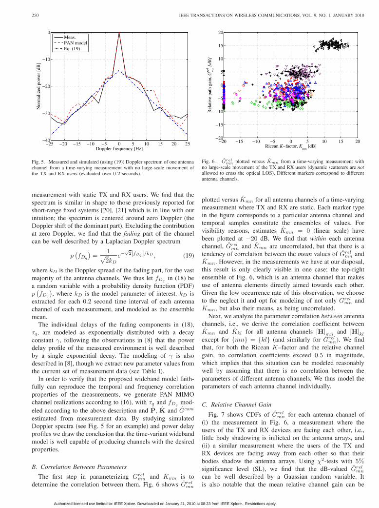
determine the correlation between them. Fig. 6 shows �̂�𝑟𝑒𝑙𝑚𝑛

−20 −15 −10 −5 0 5 10 15 20−20

−15

−10

−5

0

5

10

15

20

Ricean K−factor, Kmn

[dB]

Rel

ativ

e pa

th g

ain,

Gre

lm

n [dB

]

Fig. 6. �̂�𝑟𝑒𝑙𝑚𝑛 plotted versus �̂�𝑚𝑛 from a time-varying measurement with

no large-scale movement of the TX and RX users (dynamic scatterers are notallowed to cross the optical LOS). Different markers correspond to differentantenna channels.

plotted versus �̂�𝑚𝑛 for all antenna channels of a time-varyingmeasurement where TX and RX are static. Each marker typein the figure corresponds to a particular antenna channel andtemporal samples constitute the ensembles of values. Forvisibility reasons, estimates �̂�𝑚𝑛 = 0 (linear scale) havebeen plotted at −20 dB. We find that within each antennachannel, �̂�𝑟𝑒𝑙

𝑚𝑛 and �̂�𝑚𝑛 are uncorrelated, but that there is atendency of correlation between the mean values of �̂�𝑟𝑒𝑙

𝑚𝑛 and�̂�𝑚𝑛. However, in the measurements we have at our disposal,this result is only clearly visible in one case; the top-rightensemble of Fig. 6, which is an antenna channel that makesuse of antenna elements directly aimed towards each other.Given the low occurrence rate of this observation, we chooseto the neglect it and opt for modeling of not only 𝐺𝑟𝑒𝑙

𝑚𝑛 and𝐾𝑚𝑛, but also their means, as being uncorrelated.

Next, we analyze the parameter correlation between antennachannels, i.e., we derive the correlation coefficient between�̂�𝑚𝑛 and �̂�𝑘𝑙 for all antenna channels [H]𝑚𝑛 and [H]𝑘𝑙except for {𝑚𝑛} = {𝑘𝑙} (and similarly for �̂�𝑟𝑒𝑙

𝑚𝑛). We findthat, for both the Ricean 𝐾–factor and the relative channelgain, no correlation coefficients exceed 0.5 in magnitude,which implies that this situation can be modeled reasonablywell by assuming that there is no correlation between theparameters of different antenna channels. We thus model theparameters of each antenna channel individually.

C. Relative Channel Gain

Fig. 7 shows CDFs of �̂�𝑟𝑒𝑙𝑚𝑛 for each antenna channel of

(i) the measurement in Fig. 6, a measurement where theusers of the TX and RX devices are facing each other, i.e.,little body shadowing is inflicted on the antenna arrays, and(ii) a similar measurement where the users of the TX andRX devices are facing away from each other so that theirbodies shadow the antenna arrays. Using 𝜒2-tests with 5%significance level (SL), we find that the dB-valued �̂�𝑟𝑒𝑙

𝑚𝑛

can be well described by a Gaussian random variable. Itis also notable that the mean relative channel gain can be



−20 −15 −10 −5 0 5 10 15 200

0.1

0.2

0.3

0.4

0.5

0.6

0.7

0.8

0.9

1

Relative path gain, Grelmn

[dB]

CD

F

Low body shadowingHigh body shadowing

Fig. 7. CDFs of �̂�𝑟𝑒𝑙𝑚𝑛 for each antenna channel from two time-varying

measurements with no large-scale movement of the TX and RX users, whereasdynamic scatterers are not allowed to cross the optical LOS. One measurementhas the users of TX and RX facing each other (i.e., low body shadowing)whereas the other has the users facing away from each other (i.e., high bodyshadowing).

quite different for different antenna channels, whereas thecorresponding standard deviation (STD) is fairly constant. Wethus let

10 log10𝐺𝑟𝑒𝑙𝑚𝑛 ∼ 𝒩 (

𝜇𝐺𝑚𝑛, 𝜎𝐺), (20)

where we model 𝜇𝐺𝑚𝑛 as a Gaussian random variable (verifiedby another 𝜒2-test with 5% SL) such that

𝜇𝐺𝑚𝑛 ∼ 𝒩 (0, 𝜎𝜇𝐺

). (21)

Note that the realizations of 𝜇𝐺𝑚𝑛 should be adjusted to∑𝑚𝑛 𝜇

𝐺𝑚𝑛 = 0 in order to uphold the definition of 𝐺𝑟𝑒𝑙 and

𝐺𝑐𝑜𝑚. It is furthermore interesting to note that Fig. 7 suggeststhat 𝜇𝐺𝑚𝑛 is affected by the amount of body shadowing; thevariance of 𝜇𝐺𝑚𝑛 is much smaller in the case of large bodyshadowing than when no shadowing prevails. However, ourmeasurement data do not allow for a complete model of thisobservation and we thus have to relegate the matter to futureinvestigations.

With no large-scale movement of TX and RX and assuminga constant shadowing level, we regard 𝐺𝑟𝑒𝑙

𝑚𝑛 as a stationarystochastic process described by its autocorrelation function𝜌𝐺 (Δ𝑡). Fig. 8 shows 𝜌𝐺 (Δ𝑡) evaluated for the “high bodyshadowing” measurement of Fig. 7. We find an exponentialautocorrelation function

𝜌𝐺𝑚𝑛 (Δ𝑡) = exp

{− Δ𝑡

𝑘𝐺𝑚𝑛ln 2

}, (22)

where 𝑘𝐺𝑚𝑛 is the 50% coherence time, suitable to describethis process. Since the coherence time shows large variationsbetween different antenna channels, it seems suitable to modelit as a random variable. Showing no correlation to other modelparameters, we find (using a 𝜒2-test with 5% SL) that 𝑘𝐺𝑚𝑛can be well described by a lognormal PDF, such that

10 log10 𝑘𝐺𝑚𝑛 ∼ 𝒩 (𝜇𝑘𝐺 , 𝜎𝑘𝐺 ) . (23)

0 0.1 0.2 0.3 0.4 0.5 0.6 0.7 0.8 0.9 10

0.1

0.2

0.3

0.4

0.5

0.6

0.7

0.8

0.9

1

Temporal increment, Δt [s]

Tem

pora

l aut

ocor

rela

tion,

ρG

(Δt)

Fig. 8. Temporal autocorrelation of �̂�𝑟𝑒𝑙𝑚𝑛 from a time-varying measurement

with no large-scale movement of the TX and RX users, dynamic scatterersnot allowed to cross the optical LOS and high body shadowing level.

−20 −15 −10 −5 0 5 10 15 200

0.1

0.2

0.3

0.4

0.5

0.6

0.7

0.8

0.9

1

Ricean K−factor, Kmn

[dB]

CD

F

Fig. 9. CDFs of �̂�𝑚𝑛 for each antenna channel from a time-varyingmeasurement with no large-scale movement of the TX and RX users, whereasdynamic scatterers are not allowed to cross the optical LOS. Users of TX andRX are facing each other, i.e., low body shadowing is inflicted on the antennaarrays.

D. Ricean 𝐾–factor

Fig. 9 plots the CDFs of the 𝐾𝑚𝑛 estimates from Fig. 6. Itis notable that the probability of an antenna channel beingRayleigh distributed (𝐾 = 0) is very different betweenantenna channels, and it seems suitable to distinguish betweencases when 𝐾 = 0 and 𝐾 ∕= 0 (linear scale).9 We there-fore model 𝐾𝑚𝑛 as a Markov process with two states, S0(“Rayleigh state,” 𝐾 = 0) and S1 (“Ricean state,” 𝐾 ∕= 0), andtransition probabilities 𝛼𝑚𝑛 = Pr {𝑆1∣𝑆0} (the probabilityof shifting to S1 while in S0) and 𝛽𝑚𝑛 = Pr {𝑆0∣𝑆1} (theprobability of shifting to S0 while in S1).10 In state S0, 𝐾𝑚𝑛

9Even though there is in principle little difference between 𝐾 = 0 and a“very low” 𝐾-factor, the large concentration at 𝐾 = 0 makes this distinctionsuitable compared to using only one PDF.

10In the sequel, we give these probabilities relative our temporal sampling,i.e., 5× 18.9 = 94.7ms



−20 −15 −10 −5 0 5 10 15 200

0.1

0.2

0.3

0.4

0.5

0.6

0.7

0.8

0.9

1T

rans

ition

pro

babi

lity

Mean of K−factor, μKmn

[dB]

Pr{S0|S1}Pr{S1|S0}

−0.053μKmn

+ 0.15

Fig. 10. The transition probabilities 𝛼𝑚𝑛 = 𝑃𝑟 {𝑆1∣𝑆0} and 𝛽 =𝑃𝑟 {𝑆0∣𝑆1} plotted versus the mean of �̂�𝑚𝑛 while in state S1.

is thus constant, whereas in state S1, we find that the dB-valued 𝐾𝑚𝑛 can be reasonably well described (using 𝜒2-testswith 1% SL) by a Gaussian random variable such that

10 log10𝐾𝑚𝑛 ∼ 𝒩 (𝜇𝐾𝑚𝑛, 𝜎𝐾

), (24)

where the standard deviation 𝜎𝐾 is constant since it showsonly small variations between antenna channels. Similar to𝜇𝐺𝑚𝑛, we let 𝜇𝐾𝑚𝑛 be a Gaussian random variable (verified bya 5% 𝜒2-test), such that

𝜇𝐾𝑚𝑛 ∼ 𝒩 (𝜇𝜇𝐾 , 𝜎𝜇𝐾

). (25)

Furthermore, we note that the transition probability 𝛽𝑚𝑛shows a strong correlation with 𝜇𝐾𝑚𝑛 (see Fig. 10), whichimplies that a strongly Ricean antenna channel is less proneof shifting to the Rayleigh state. We find this well describedby a deterministic relationship

𝛽𝑚𝑛(𝜇𝐾𝑚𝑛

)=

⎧⎨⎩

1, 𝜇𝐾𝑚𝑛 < −16−0.053𝜇𝐾𝑚𝑛 + 0.15, −16 ≤ 𝜇𝐾𝑚𝑛 ≤ 2.80, 𝜇𝐾𝑚𝑛 > 2.8,

(26)such that the probability of shifting to the Rayleigh state iszero if the antenna channel is “Ricean enough.” The transitionprobability 𝛼𝑚𝑛, on the other hand, shows no correlation with𝜇𝐾𝑚𝑛, but is better described by a random variable. Using a𝜒2-test with 5% SL, we find that a uniform distribution

𝛼𝑚𝑛 ∼ 𝒰 (0.23, 0.72) (27)

constitutes a good description.For the same reasons mentioned in Sec. V-C, we can regard

𝐾𝑚𝑛 as a stationary stochastic process while in state S1. Here,the temporal autocorrelation of �̂�𝑚𝑛, 𝜌𝐾 (Δ𝑡), can only bedetermined when �̂�𝑚𝑛 is in the S1 state during a sufficientlylong time period, which reduces the statistical ensemblesomewhat. We find that also in this case, an exponentialautocorrelation function

𝜌𝐾𝑚𝑛 (Δ𝑡) = exp

{− Δ𝑡

𝑘𝐾𝑚𝑛ln 2

}, (28)

is suitable, where the 50% coherence time 𝑘𝐾𝑚𝑛 is welldescribed by a lognormal PDF (verified by a 𝜒2-test with 5%SL), such that

10 log10 𝑘𝐾𝑚𝑛 ∼ 𝒩 (

𝜇𝑘𝐾𝑚𝑛, 𝜎𝑘𝐾𝑚𝑛

). (29)

VI. IMPLEMENTATION RECIPE

Channel realizations of an 𝑀 ×𝑁 MIMO system can thusbe generated according to our parameterized model as follows:

1) Select a suitable time window and frequency band forthe simulations and select the sampling grid in time andfrequency.

2) Determine the large-scale shadowing 𝐺𝑐𝑜𝑚 containingdistance-dependent decay, shadowing due to environ-ment and body shadowing. Determine at the sametime, for each antenna channel, the decay constant ofthe power delay profile 𝛾𝑚𝑛 since this parameter iscorrelated with the shadowing. These parameters aredescribed in detail in [8] and have therefore not beencovered in the current paper.

3) Determine the angle-of-arrival, 𝜃𝑟, and angle-of-departure, 𝜃𝑡, of the dominant component from 𝒰 [0, 2𝜋).

4) Determine, for each antenna channel, the parameters ofthe stochastic processes 𝐺𝑟𝑒𝑙

𝑚𝑛 (𝑡): (i) the mean 𝜇𝐺𝑚𝑛 from(21) and (ii) the coherence time 𝑘𝐺𝑚𝑛 from (23).

5) Derive, for each antenna channel, the temporal realiza-tions of 𝐺𝑟𝑒𝑙

𝑚𝑛 (𝑡) from (20) and (22).6) Determine, for each antenna channel, the parameters of

the stochastic processes 𝐾𝑚𝑛 (𝑡): (i) the S1 mean 𝜇𝐾𝑚𝑛from (25), (ii) the S1 coherence time 𝑘𝐾𝑚𝑛 from (29) and(iii) the transition probabilities 𝛼𝑚𝑛 and 𝛽𝑚𝑛 from (27)and (26), respectively.

7) Derive, for each antenna channel, the temporal realiza-tions of 𝐾𝑚𝑛 (𝑡). Start in S1 if 𝛼𝑚𝑛 > 𝛽𝑚𝑛 and in S0otherwise. For each time instant, test if a state transitionshould be made. While remaining in S1, determine𝐾𝑚𝑛 (𝑡) from (24) and (28) until the next state is S0.When changing from S0 to S1, start a new time seriesof 𝐾𝑚𝑛 (𝑡), i.e., disregard any correlation to previousrealizations.

8) Derive the matrices P and K from (5) and (6), respec-tively.

9) Derive, for each antenna channel, the fading channelimpulse response from (18) using 𝛾𝑚𝑛 to derive 𝜏𝑞 and𝑘𝐷 to derive 𝑓𝐷𝑞 from (19). A Fourier transform createsthe corresponding frequency response

[H𝑓𝑑 (𝑓, 𝑡)

]𝑚𝑛

.10) Derive, for each antenna channel, the dominant chan-

nel impulse response from (17) and derive the corre-sponding frequency response

[H𝑑𝑚 (𝑓, 𝑡)

]𝑚𝑛

through aFourier transform.

11) Derive the complete 𝑀 ×𝑁 time-varying channel fre-quency response H (𝑓, 𝑡) from (16).

The model parameters 𝜎𝐺, 𝜎𝜇𝐺 , 𝜇𝑘𝐺 , 𝜎𝑘𝐺 , 𝜎𝐾 , 𝜇𝜇𝐾 , 𝜇𝜇𝐾 ,𝜎𝜇𝐾 , 𝜇𝑘𝐾 , 𝜎𝑘𝐾 , 𝑘𝐷, 𝜇𝛾 , and 𝜎𝛾 are given in Table I.

VII. PARAMETERIZATION VALIDATION

In this section we investigate the suitability of the modelparameterization in terms of its capability to reproduce MIMO



TABLE IMODEL PARAMETERS.

Process Description Notation Value Unit

𝐺𝑟𝑒𝑙𝑚𝑛

STD 𝜎𝐺 1.3 dBSTD of mean 𝜎𝜇𝐺 3.7 dBMean of coherence time 𝜇𝑘𝐺

3.2 dBsSTD of coherence time 𝜎𝑘𝐺

6.8 dBs

𝐾𝑚𝑛

STD 𝜎𝐾 4.0 dBMean of mean 𝜇𝜇𝐾 −0.2 dBSTD of mean 𝜎𝜇𝐾 2.6 dBMean of coherence time 𝜇𝑘𝐾

3.9 dBsSTD of coherence time 𝜎𝑘𝐾

6.3 dBs

𝑓𝐷𝑞 Doppler spread (fd) 𝑘𝐷 5.7 Hz

𝛾Mean of decay constant (fd) 𝜇𝛾 −79 dBsSTD of decay constant (fd) 𝜎𝛾 0.5 dBs

0 5 10 15 200

0.1

0.2

0.3

0.4

0.5

0.6

0.7

0.8

0.9

1

rms delay spread [ns]

CD

F

Meas.Par. model

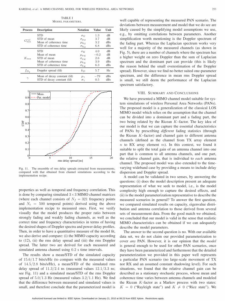
Fig. 11. The ensemble of rms delay spreads extracted from measurements,compared with that obtained from channel simulations according to theimplementation recipe.

properties as well as temporal and frequency correlation. Thisis done by comparing simulated 3×3 MIMO channel matrices(where each channel consists of 𝑁𝑓 = 321 frequency pointsand 𝑁𝑡 = 500 temporal points) derived using the aboveimplementation recipe to measured ones. First, we verifyvisually that the model produces the proper ratio betweenstrongly fading and weakly fading channels, as well as thecorrect time and frequency characteristics in terms of havingthe desired shapes of Doppler spectra and power delay profiles.Then, in order to have a quantitative measure of the model fit,we also derive and compare: (i) the MIMO capacity accordingto (12), (ii) the rms delay spread and (iii) the rms Dopplerspread. The latter two are derived for each measured andsimulated antenna channel using 0.2 s time intervals.

The results show a mean/STD of the simulated capacityof 15.6/1.7 bits/s/Hz (to compare with the measured valuesof 14.5/2.8 bits/s/Hz), a mean/STD of the simulated rmsdelay spread of 11.3/2.4 ns (measured values 12.1/3.3 ns;see Fig. 11) and a simulated mean/STD of the rms Dopplerspread of 5.0/1.3 Hz (measured values 3.2/1.1 Hz). We findthat the difference between measured and simulated values issmall, and therefore conclude that the parameterized model is

well capable of representing the measured PAN scenario. Thedeviations between measurement and model that we do see arelikely caused by the simplifying model assumptions we use,e.g., by omitting correlations between parameters. Anothersimplification worth mentioning is the Doppler spectrum ofthe fading part. Whereas the Laplacian spectrum works verywell for a majority of the measured channels (as shown inFig. 5), there are a number of channels where the spectrum hasa higher weight on zero Doppler than the sum of Laplacianspectrum and the dominant part can provide (this is likelythe reason behind the small overestimation of the Dopplerspread). However, since we find no better suited one-parameterspectrum, and the difference in mean rms Doppler spreadis small, we still deem the performance of the Laplacianspectrum satisfactory.

VIII. SUMMARY AND CONCLUSIONS

We have presented a MIMO channel model suitable for sys-tem simulations of wireless Personal Area Networks (PANs).The proposed model is a generalization of the classical LOSMIMO model which relies on the assumption that the channelcan be divided into a dominant part and a fading part, thetwo being related by the Ricean 𝐾–factor. The key idea ofour model is that we can capture the essential characteristicsof PANs by prescribing different fading statistics (throughthe Ricean 𝐾–factor) and channel gain to different antennachannels (defined as the channel from TX array element𝑛 to RX array element 𝑚). In this context, we found itsuitable to split the total gain of an antenna channel into onepart that is common to all antenna channels, and one part,the relative channel gain, that is individual to each antennachannel. The proposed model was also extended to the time-varying wideband case by providing a means to include delaydispersion and Doppler spread.

A model can be validated in two senses, by answering thequestions: (i) does the model description present an adequaterepresentation of what we seek to model, i.e., is the modelcomplexity high enough to capture the desired effects, and(ii) is the model parameterization representative to describe themeasured scenarios in general? To answer the first question,we compared simulated results on capacity, eigenvalue distri-bution and antenna correlation to those derived from severalsets of measurement data. From the good match we obtained,we concluded that our model is valid in the sense that realisticMIMO characteristics can be obtained if we can adequatelydescribe the model parameters.

The answer to the second question is no. With our availabledata set, we do not claim our provided parameterization tocover any PAN. However, it is our opinion that the modelis general enough to be used for other PAN scenarios, oncethey have been parameterized and furthermore that the detailedparameterization we provided in this paper well representsa particular PAN scenario (no large-scale movement of TXnor RX and an assumed constant shadowing level). For suchsituations, we found that the relative channel gain can bedescribed as a stationary stochastic process, whose mean andcoherence time varies between antenna channels and modeledthe Ricean 𝐾-factor as a Markov process with two states:𝐾 = 0 (“Rayleigh state”) and 𝐾 ∕= 0 (“Rice state”). We



described the transition probabilities and found that while inthe Rice state, 𝐾 can be modeled as a stationary stochasticprocess, with different mean and coherence time for differentantenna channels.

The paper was rounded off by an implementation recipe andthus provides everything that is needed to be used in systemsimulations, though the model parameterization is obviouslybest suited for situations similar to those covered by ourmeasurements. Some correlative effects (e.g., the connectionbetween relative channel gain variance and shadowing, or thecorrelation between the relative channel gain and the Ricean𝐾-factor), could not be fully investigated due the limitednumber of measurements and are thus amongst the mattersconstituting a good basis for future investigations.

ACKNOWLEDGMENTS

We thank Bristol University, especially Prof. Mark Beach,for kindly lending us their antennas.

REFERENCES

[1] D. Bakker, D. M. Gilster, and R. Gilster, Bluetooth End to End, 1st ed.Wiley, 2002.

[2] A. Batra et al., “Multi-band OFDM physical layer proposal," 2003,document IEEE 802.15-03/267r2.

[3] J. H. Winters, “On the capacity of radio communications systemswith diversity in Rayleigh fading environments," IEEE J. Sel. AreasCommun., vol. 5, no. 5, pp. 871-878, June 1987.

[4] G. J. Foschini and M. J. Gans, “On limits of wireless communications ina fading environment when using multiple antennas," Wireless PersonalCommun., vol. 6, pp. 311-335, Feb. 1998.

[5] A. Paulraj, D. Gore, and R. Nabar, Multiple Antenna Systems. Cam-bridge, U.K.: Cambridge University Press, 2003.

[6] [Online]. Available: http://web.archive.org/web/20071024180734/http://www.ist-magnet.org/.

[7] A. F. Molisch, Wireless Communications. Chichester, West Sussex, UK:IEEE Press–Wiley, 2005.

[8] J. Karedal, A. J. Johansson, F. Tufvesson, and A. F. Molisch, “Ameasurement-based fading model for wireless personal area networks,"IEEE Trans. Wireless Commun., vol. 7, no. 11, pp. 4575-4585, Nov.2008.

[9] P. Almers, E. Bonek, A. Burr, N. Czink, M. Debbah, V. Degli-Esposti, H. Hofstetter, P. Kyoesti, D. Laurenson, G. Matz, A. Molisch,C. Oestges, and H. Oezcelik, “Survey of channel and radio propagationmodels for wireless MIMO systems," EURASIP J. Wireless Commun.Networking, vol. 2007.

[10] J. P. Kermoal, L. Schumacher, K. I. Pedersen, P. E. Mogensen, andF. Frederiksen, “A stochastic MIMO radio channel model with exper-imental validation," IEEE J. Sel. Areas Commun., vol. 20, no. 6, pp.1211-1226, Aug. 2002.

[11] D. P. McNamara, M. A. Beach, and P. N. Fletcher, “Spatial correlationin indoor MIMO channels," in Proc. IEEE Int. Symp. Personal, Indoor,Mobile Radio Commun., vol. 1, Lisbon, Portugal, 2002, pp. 290-294.

[12] A. M. Sayeed, “Deconstructing multiantenna fading channels," IEEETrans. Signal Process., vol. 50, no. 10, pp. 2563-2579, Oct. 2002.

[13] W. Weichselberger, M. Herdin, H. Özcelik, and E. Bonek, “A stochasticMIMO channel model with joint correlation of both link ends," IEEETrans. Wireless Commun., vol. 5, no. 1, pp. 90-100, Jan. 2006.

[14] M. Shafi, M. Zhang, A. L. Moustakas, P. J. Smith, A. F. Molisch,F. Tufvesson, and S. H. Simon, “Polarized MIMO channels in 3-D:models, measurements and mutual information," IEEE J. Sel. AreasCommun., vol. 24, no. 3, pp. 514-527, Mar. 2006.

[15] M. Coldrey, “Modeling and capacity of polarized MIMO channels," inProc. IEEE Veh. Technol. Conf. 2008 Spring, Singapore, May 2008, pp.440-444.

[16] F. Rashid-Farrokhi, A. Lozano, G. Foschini, and R. Valenzuela, “Spec-tral efficiency of wireless systems with multiple transmit and receiveantennas," in Proc. IEEE Int. Symp. Personal, Indoor, Mobile RadioCommun., vol. 1, Sep. 2000, pp. 373-377.

[17] R. Thomae, D. Hampicke, A. Richter, G. Sommerkorn, A. Schneider,U. Trautwein, and W. Wirnitzer, “Identification of the time-variantdirectional mobile radio channels," IEEE Trans. Instrum. Meas., vol. 49,no. 2, pp. 357-364, Sep. 2000.

[18] C. Tepedelenlioglu, A. Abdi, and G. B. Giannakis, “The Ricean K factor:estimation and performance analysis," IEEE Trans. Wireless Commun.,vol. 2, no. 4, pp. 799-810, July 2003.

[19] P. Hoeher, “A statistical discrete-time model for the WSSUS multipathchannel," IEEE Trans. Veh. Technol., vol. 41, no. 4, pp. 461-468, Nov.1992.

[20] A. Domazetovic, L. J. Greenstein, N. B. Mandayam, and I. Seskar,“Estimating the Doppler spectrum of a short-range fixed wirelesschannel," IEEE Commun. Lett., vol. 7, no. 5, pp. 227-229, May 2003.

[21] P. Pagani and P. Pajusco, “Characterization and modeling of temporalvariations on an ultrawideband radio link," IEEE Trans. AntennasPropag., vol. 54, no. 11, pp. 3198-3206, Nov. 2006.

Johan Karedal received his M.S. degree in en-gineering physics in 2002 and his Ph.D. in radiocommunications in 2009, both from Lund Univer-sity, Sweden. He is currently a postdoctoral fellow atthe Department of Electrical and Information Tech-nology, Lund University, where his main researchinterests concern measurements and modeling ofthe wireless propagation channel for MIMO andUWB systems. Dr. Karedal has participated in theEuropean research initiative “MAGNET.”

Peter Almers received the M.S. degree in electricalengineering in 1998 and his Ph.D. degree in 2007,both from Lund University, Sweden. Currently heis a senior staff engineer at ST-Ericsson, Lund,Sweden. Between 1998 and 2006, he was also withthe radio research department at TeliaSonera AB(formerly Telia AB), in Malmö, Sweden, mainlyworking with WCDMA and 3GPP standardizationphysical layer issues. From 2007 to 2008, he workedas a research fellow at the Department of Electricaland Information Technology, Lund University.

Dr. Almers has participated in the European research initiatives“COST273,” the European network of excellence “NEWCOM” and theNORDITE project “WILATI.” He received an IEEE Best Student Paper Awardat PIMRC in 2002.

Anders J Johansson received his M.S., Lic. Eng.and Ph.D. degrees in electrical engineering fromLund University, Lund, Sweden, in 1993, 2000 and2004 respectively. From 1994 to 1997 he was withEricsson Mobile Communications AB developingtransceivers and antennas for mobile phones. Since2005 he is an Associate Professor at the Departmentof Electrical and Information Technology, LundUniversity. His research interests include antennas,wave propagation and telemetric devices for medicalimplants as well as antenna systems and propagation

modelling for MIMO systems.

Fredrik Tufvesson was born in Lund, Sweden in1970. He received the M.S. degree in electricalengineering in 1994, the Licentiate Degree in 1998and his Ph.D. in 2000, all from Lund Universityin Sweden. After almost two years at a startupcompany, Fiberless Society, Fredrik is now asso-ciate professor at the Department of Electrical andInformation Technology. His main research interestsare channel measurements and modeling for wirelesscommunication, including channels for both MIMOand UWB systems. Beside this, he also works with

channel estimation and synchronization problems, OFDM system design andUWB transceiver design.



Andreas F. Molisch received the Dipl. Ing., Dr.techn., and habilitation degrees from the TechnicalUniversity Vienna (Austria) in 1990, 1994, and1999, respectively. From 1991 to 2000, he was withthe TU Vienna, becoming an associate professorthere in 1999. From 2000 to 2002, he was with theWireless Systems Research Department at AT&T(Bell) Laboratories Research in Middletown, NJ.From 2002 to 2008, he was with Mitsubishi Elec-tric Research Labs, Cambridge, MA, USA, mostrecently as Distinguished Member of Technical Staff

and Chief Wireless Standards Architect. Concurrently he was also Professorand Chairholder for radio systems at Lund University, Sweden. Since 2009,he is Professor of Electrical Engineering and Head of the Wireless Devicesand Systems (WiDeS) group at the University of Southern California, LosAngeles, CA, USA.

Dr. Molisch has done research in the areas of SAW filters, radiative transferin atomic vapors, atomic line filters, smart antennas, and wideband systems.His current research interests are measurement and modeling of mobileradio channels, UWB, cooperative communications, and MIMO systems. Dr.

Molisch has authored, co-authored or edited four books (among them thetextbook Wireless Communications, Wiley-IEEE Press); 11 book chapters,more than 120 journal papers, and numerous conference contributions, aswell as more than 70 patents and 60 standards contributions.

Dr. Molisch is Area Editor for Antennas and Propagation of the IEEETRANSACTIONS ON WIRELESS COMMUNICATIONS and co-editor of specialissues of several journals. He has been member of numerous TPCs, vice chairof the TPC of VTC 2005 spring, general chair of ICUWB 2006, TPC co-chairof the wireless symposium of Globecomm 2007, TPC chair of Chinacom2007,and general chair of Chinacom 2008. He has participated in the Europeanresearch initiatives “COST 231,” “COST 259,” and “COST273,” where hewas chairman of the MIMO channel working group, he was chairman ofthe IEEE 802.15.4a channel model standardization group. From 2005 to2008, he was also chairman of Commission C (signals and systems) of URSI(International Union of Radio Scientists), and since 2009, he is the Chair of theRadio Communications Committee of the IEEE Communications Society. Dr.Molisch is a Fellow of the IEEE, a Fellow of the IET, an IEEE DistinguishedLecturer, and recipient of several awards.


Documents

A MIMO channel model for wireless personal area networks ...lup.lub.lu.se/search/ws/files/4272138/1530432.pdf · Fredrik Tufvesson, Senior Member, IEEE, and Andreas F. Molisch, Fellow,