Embed Size (px)
Citation preview

1. Report No. FHWA/TX-09/0-5261-2
2. Government Accession No.
3. Recipient's Catalog No.
4. Title and Subtitle A METHOD FOR PREDICTING ASPHALT MIXTURE COMPACTABILITY AND ITS INFLUENCE ON MECHANICAL PROPERTIES
5. Report Date December 2008 Published: May 2009 6. Performing Organization Code
7. Author(s) Eyad Masad, Emad Kassem, Arif Chowdhury, and Zhanping You
8. Performing Organization Report No. Report 0-5261-2
9. Performing Organization Name and Address Texas Transportation Institute The Texas A&M University System College Station, Texas 77843-3135
10. Work Unit No. (TRAIS) 11. Contract or Grant No. Project 0-5261
12. Sponsoring Agency Name and Address Texas Department of Transportation Research and Technology Implementation Office P. O. Box 5080 Austin, Texas 78763-5080
13. Type of Report and Period Covered Technical Report: January 2008-August 2008 14. Sponsoring Agency Code
15. Supplementary Notes Project performed in cooperation with the Texas Department of Transportation and the Federal Highway Administration. Project Title: Using Imaging Analysis Technology to Improve the Laboratory and Field Compaction of HMA URL: http://tti.tamu.edu/documents/0-5261-2.pdf 16. Abstract
This project aimed at providing better understanding of the factors affecting the uniformity and level of compaction; and the performance of asphalt pavements. TxDOT research report 0-5261-1 documented some of the findings of this research project. This research report documents the efforts and findings of experiments conducted with more test sections. In the first phase of this report, a number of field test sections were compacted, and field cores were extracted. These cores were scanned using X-ray Computed Tomography (X-ray CT) to capture the air void distributions in these cores. The air void distribution correlated well with the compaction effort across the mat. The compaction effort was found to be a function of the number of roller passes and the relative location of each pass across the mat. The Compaction Index (CI) developed in the TxDOT research report 0-5261-1 was used to quantify the compaction effort at any point in the pavement. This index combines the number of roller passes along with the effectiveness of each pass on the mat. The compactability of asphalt mixtures in the field correlated well with compactability of asphalt mixtures in the laboratory. The CI was used to quantify the compactability of asphalt mixtures in the field while the slope of the compaction curves obtained from Superpave Gyratory Compactor was used to quantify the compactability of asphalt mixtures in the laboratory. In the second phase of this report, the effect of different levels of compaction on the performance of asphalt mixtures was studied using a fracture mechanics approach and DEM models. The results showed that test specimens with less percent air voids performed better than the ones with higher percent air voids. In addition moisture-conditioned specimens performed worse than the dry ones at the same compaction levels. Furthermore, guidelines were developed to assist in predicting the compactability in the field based on laboratory measurements during the mixture design stage; and to improve the field compaction. 17. Key Words Hot-Mix Asphalt, Compaction, Effectiveness Factor, Uniformity, X-ray CT, HMA Moisture Susceptibility, DEM
18. Distribution Statement No restrictions. This document is available to the public through NTIS: National Technical Information Service Springfield, Virginia 22161 http://www.ntis.gov
19. Security Classif. (of this report) Unclassified
20. Security Classif. (of this page) Unclassified
21. No. of Pages 98
22. Price


A METHOD FOR PREDICTING ASPHALT MIXTURE COMPACTABILITY AND ITS INFLUENCE ON MECHANICAL
PROPERTIES
by
Eyad Masad Associate Research Scientist
Texas Transportation Institute
Emad Kassem Assistant Research Scientist
Texas Transportation Institute
Arif Chowdhury Assistant Research Engineer
Texas Transportation Institute
and
Zhanping You Associate Professor
Michigan Technological University
Report 0-5261-2 Project 0-5261
Project Title: Using Imaging Analysis Technology to Improve the Laboratory and Field Compaction of HMA
Performed in cooperation with the Texas Department of Transportation
and the Federal Highway Administration
December 2008 Published: May 2009
TEXAS TRANSPORTATION INSTITUTE The Texas A&M University System College Station, Texas 77843-3135


v
DISCLAIMER
The contents of this report reflect the views of the authors, who are responsible
for the facts and the accuracy of the data presented herein. The contents do not
necessarily reflect the official view or policies of the Texas Department of Transportation
(TxDOT) or the Federal Highway Administration (FHWA). This report does not
constitute a standard, specification, or regulation. The engineer in charge of the project
was Eyad A. Masad, Texas #96368.

vi
ACKNOWLEDGMENTS
The authors wish to express their appreciation to the Texas Department of
Transportation personnel for their support throughout this project, as well as the Federal
Highway Administration. We would also like to thank the project director Dr. German
Claros and the members of the project monitoring committee, Mr. Ed Oshinski, Mr.
Magdy Mikhail, and Ms. Darlene Goehl for their valuable technical comments during this
project. The co-operation from participating TxDOT district personnel for their support
during field testing are highly appreciated by the authors.

vii
TABLE OF CONTENTS Page
LIST OF FIGURES .............................................................................................................x
LIST OF TABLES ........................................................................................................... xiii
CHAPTER 1 INTRODUCTION AND BACKGROUND .................................................1 OVERVIEW ..............................................................................................................1
PROBLEM STATEMENT AND OBJECTIVES ......................................................2
STUDY PLAN ...........................................................................................................3
Task 1: Conduct Field Compaction ....................................................................3
Task 2: Analyze Air Void Distribution ..............................................................4 Task 3: Evaluate Field Compactability and Laboratory Compactability ...........4 Task 4: Use Fracture Mechanics Approach to Assess Moisture Damage ..........5 Task 5: Use DEM to Study Effect of Air Void on Mechanical
Properties of Asphalt Mixtures ...........................................................................5 Task 6: Develop Guideline for Improving Field Compaction ...........................5
ORGANIZATION OF REPORT ...............................................................................5
CHAPTER 2 EVALUATION OF FIELD COMPACTION ..............................................7 INTRODUCTION .....................................................................................................7 DESCRIPTION OF TEST SECTIONS .....................................................................7
SH 6 in Bryan District ........................................................................................7 SH 44 in Laredo District ....................................................................................8 SL 1 in Austin District ........................................................................................9
RELATIONSHIP BETWEEN COMPACTION EFFORT AND
PERCENT AIR VOIDS ...........................................................................................10 APPLICATIONS OF THE COMPACTION INDEX .............................................17 COMPARISON OF LABORATORY AND FIELD MECHANICAL
PROPERTIES ..........................................................................................................24 EFFECT OF THE AIR VOID DISTRIBUTION ON THE HAMBURG
TEST ........................................................................................................................25 CONCLUSIONS ......................................................................................................28

viii
CHAPTER 3 FRACTURE-BASED ANALYSIS OF INFLUENCE OF
AIR VOIDS ON MOISTURE DAMAGE ........................................................................29
INTRODUCTION AND OBJECTIVES .................................................................29
ASPHALT MIXTURES TEST SPECIMENS .........................................................29
MOISTURE CONDITIONING ...............................................................................31
EXPERIMENTAL TESTS ......................................................................................31
Relaxation Test ..................................................................................................31
Dynamic Direct Tension Test ............................................................................34
Tensile Strength Test .........................................................................................38
Surface Energy Measurements .........................................................................39
CRACK GROWTH FRACTURE MODEL .............................................................40
EXPERIMENTAL TEST RESULTS ......................................................................41
Results of Tensile Relaxation Test .....................................................................41
Results of Dynamic Direct Tension Test ............................................................42
Results of Tensile Strength Test .........................................................................46
Results of Adhesive Bond Energy ......................................................................48
RESULTS AND ANALYSIS .................................................................................49
SUMMARY .............................................................................................................51
CHAPTER 4 DISCRETE ELEMENT MODELS OF MECHANICAL
PROPERTIES OF ASPHALT MIXTURES ....................................................................53
INTRODUCTION ...................................................................................................53
SCOPE .....................................................................................................................53
BACKGROUND OF MICROMECHANICAL MODELS .....................................53
TEST SPECIMENS AND X-RAY CT ....................................................................54
MICROMECHANICAL MODEL DESCRIPTION ................................................56
DEM SIMULATION OF BIAXIAL TEST AND TRIAXIAL TEST .....................56
MICROSTRUCTURE RECONSTRUCTION .......................................................59
3D MODEL PREPARATION .................................................................................60
2D DEM SIMULATION TO SHOW THE EFFECTS OF THE VERTICAL
ORIENTATION ......................................................................................................60

ix
2D DEM SIMULATION TO SHOW THE EFFECTS OF THE
HORIZONTAL ORIENTATION ............................................................................61
COMPARE 3D MODELS, 2D VERTICAL ORIENTATION MODELS,
AND 2D HORIZONTAL ORIENTATION MODELS ...........................................63
AIR VOID ORIENTATION EFFECT ....................................................................65
SUMMARY AND CONCLUSIONS ......................................................................69
CHAPTER 5 GUIDELINE FOR IMPROVING FIELD COMPACTION .......................71 INTRODUCTION ...................................................................................................71 RECOMMENDATIONS DURING THE MIXTURE DESIGN STAGE ...............71 RECOMMENDATIONS DURING THE CONSTRUCTION STAGE ..................74
CHAPTER 6 CONCLUSIONS AND RECOMMENDATIONS .....................................75 CONCLUSIONS.......................................................................................................75
Evaluation of Field Compaction ........................................................................75 Fracture Analysis of Moisture Damage .............................................................76 Discrete Element Models of Mechanical Properties ..........................................76
RECOMMENDATIONS ..........................................................................................76
REFERENCES .................................................................................................................79

x
LIST OF FIGURES FIGURE Page
2-1 Coring Layout on SH 6 ...........................................................................................9
2-2 Application of Prime Coat on Flexible Base .........................................................10
2-3 Number of Passes and the Percent of Air Voids across the Mat in
SH 6 Test Section ..................................................................................................11
2-4 Number of Passes and the Percent of Air Voids across the Mat in
SH 44 Test Section ................................................................................................11
2-5 Number of Passes and the Percent of Air Voids across the Mat in
SL 1 Test Section ..................................................................................................12
2-6 Effectiveness Distribution across Roller Width ....................................................13
2-7 (a) Number of Passes versus the Percent of Air Voids in SH 6 Test Section,
(b) Compaction Index versus the Percent of Air Voids in SH 6 Test Section ......14
2-8 (a) Number of Passes versus the Percent of Air Voids in
SH 44 Test Section, (b) Compaction Index versus the Percent of Air Voids in
SH 44 Test Section ................................................................................................15
2-9 (a) Number of Passes versus the Percent of Air Voids in SL 1 Test Section,
(b) Compaction Index versus the Percent of Air Voids in SL 1 Test Section ......16
2-10 (a) Air Void Distribution (%) across the Mat for SH 6 Test Section,
(b) the CI and Average Percent of Air Voids across the Mat for
SH 6 Test Section ..................................................................................................18
2-11 (a) Air Void Distribution (%) across the Mat for SH 44 Test Section,
(b) the CI and Average Percent of Air Voids across the Mat for
SH 44 Test Section ................................................................................................19
2-12 (a) Air Void Distribution (%) across the Mat for SL 1 Test Section,
(b) the CI and Average Percent of Air Voids across the Mat for
SL 1 Test Section ..................................................................................................20
2-13 The CI versus the Percent of Air Voids ................................................................21
2-14 Compaction Index versus the Slope of LN (No. of Gyrations) and Percent
Air Voids Curve at 8 Percent Air Voids for Different Mixes ...............................22
xi
2-15 Air Void Distribution (%) along the Depth of the Mat for SH 6
Test Section ...........................................................................................................23
2-16 Air Void Distribution (%) along the Depth of the Mat for SH 44
Test Section ...........................................................................................................23
2-17 Air Void Distribution (%) along the Depth of the Mat for SL 1
Test Section ...........................................................................................................24
2-18 The Average, Top, and Bottom Percent of Air Voids for Different Cases ...........27
2-19 Hamburg Test Results for Different Cases ...........................................................27
3-1 0.45 Power Aggregate Gradation Chart ................................................................30
3-2 Applied Load during the Relaxation Test .............................................................32
3-3 Schematic View of LVDTs Configurations .........................................................33
3-4 LVDTs Configuration ...........................................................................................34
3-5 Applied Loading Configurations for Dynamic Direct Tension Test ....................35
3-6 An Example of Measured Stress vs. Pseudostrain ................................................37
3-7 Normalized DPSE, WR vs. Number of Cycles .....................................................37
3-8 Test Sample after Failure inside the MTS ............................................................38
3-9 Test Specimen after Failure (a) Wet Condition, (a) Dry Condition .....................39
3-10 Examples of Tensile Relaxation Test Results at Different Percent Air
Voids in Dry Conditions .......................................................................................42
3-11 Initial Tensile Relaxation Modulus Ratio versus Percent Air Voids ....................43
3-12 Normalized DPSE (WR) versus Number of Cycles at Different Percent
Air Voids ...............................................................................................................44
3-13 Intercept (a) versus Percent Air Voids in Dry Conditions ....................................44
3-14 Intercept (a) versus Percent Air Voids in Wet Conditions ...................................45
3-15 Percent Air Voids versus Slope (b) in Dry Conditions .........................................45
3-16 Percent Air Voids versus Slope (b) in Wet Conditions ........................................46
3-17 Average Tensile Strength versus Percent Air Voids in Dry Conditions ...............47
3-18 Average Tensile Strength versus Percent Air Voids in Wet Conditions ..............47
3-19 Tensile Strength Ratio versus Percent Air Voids .................................................48
3-20 Crack Growth Index at Different Percent Air Voids in Dry and
Wet Conditions ......................................................................................................50

xii
3-21 Crack Growth Index (Wet/Dry) versus Percent Air Voids ...................................50
4-1 Illustration of Image Processing and DEM Modeling Micromechanical
Model Description for Asphalt Mixture Specimens .............................................58
4-2 Vertical and Horizontal “Cut” of the X-ray Images for the 2D Vertical
and Horizontal Models ..........................................................................................59
4-3 3D Model Preparation ...........................................................................................60
4-4 Air Void of the Vertical Section of the Three Specimens (2D Models) ...............62
4-5 Normalized Modulus of the Vertical Section of Three Specimens
(2D Models) ..........................................................................................................62
4-6 Air Void of the Horizontal Section of the Specimens ..........................................63
4-7 Normalized Modulus of the Horizontal Section of the Specimens
(2D Models) ..........................................................................................................63
4-8 Normalized Modulus vs. Air Void (2D and 3D Models) .....................................66
4-9 Compare Air Void Level of the 3D, 2D Vertical Orientation, and 2D
Horizontal Orientation using X-ray CT Images ....................................................67
4-10 Compare Normalized Modulus of 3D, 2D Vertical Orientation, and 2D
Horizontal Orientation using X-ray CT Images ....................................................67
4-11 Comparing Normalized Modulus of the Idealized Images, Real Images,
and 3D Images ......................................................................................................68
5-1 Evaluating the Compactability Process ................................................................73
xiii
LIST OF TABLES TABLE Page
2-1 Summary of Mixture Designs ..................................................................................8
2-2 Description of Compaction Patterns .......................................................................8
2-3 Summary of Mechanical Tests Results .................................................................25
3-1 Aggregate Gradation of SH 87 Type C Asphalt Mixtures ....................................30
3-2 Vacuum Saturation Time ......................................................................................31
3-3 Surface Energy Components .................................................................................40
3-4 Average Parameters for the Fracture Model .........................................................49
4-1 Compaction Data of Laboratory Specimens .........................................................55
4-2 Location of Field Cores ........................................................................................56
4-3 Parameters of 2D and 3D Models .........................................................................68
5-1 Recommended Levels for Field Compactability ..................................................73


1
CHAPTER 1
INTRODUCTION AND BACKGROUND
OVERVIEW
Compaction is the process by which the volume of an asphalt mixture is reduced,
leading to an increase in unit weight of the mixture and interlock among aggregate
particles (Corps of Engineers 2000; Roberts et al. 1996). The performance of asphalt
mixtures is significantly influenced by the degree of compaction. Insufficient compaction
leads to poor asphalt pavement performance even if all desirable mixture design
characteristics are met. Poor compaction can result in premature permanent deformation
or rutting, excessive aging, and moisture damage.
There are many factors that affect the compaction process; these factors include
the properties of the materials in the mixture, environmental variables, conditions at the
lay down site, and the method of compaction. A number of studies were carried out in
order to evaluate the relationship between laboratory and field compaction methods and
mechanical properties of asphalt mixtures (Consuegra et al. 1989; Harvey and Monismith
1993; Peterson et al. 2004; Tashman et al. 2001). Based on the published literature, it can
be seen that very little effort has been devoted in the past to evaluate the effect of changes
in field compaction patterns on degree of compaction and uniformity of air void
distribution in asphalt pavements. This uniformity leads to asphalt pavements with more
uniform properties and improved performance. Additionally, there is a need to develop a
method to relate field compaction to laboratory compaction in order to predict asphalt
mixture compactability based on laboratory measurements.
The effect of the air void distribution on moisture diffusion, as an important cause
of moisture damage in asphalt pavements, also needs to be investigated. Most studies
have focused on permeability as a measure of the infiltration of water in the mixture
(Masad et al. 2006a). However, evidence of severe moisture damage in pavements in
areas with low levels of annual rainfall, such as Arizona and New Mexico (Caro et al.
2007), implies that the diffusion of water vapor could be an important source of moisture
damage in pavements. The diffusion coefficient is an important input for modeling
moisture transport and predicting moisture damage in asphalt mixtures. Developing an

2
experimental procedure for measuring the diffusion coefficient of asphalt mixtures and
evaluating the effect of the air void distribution on the moisture diffusion is one of the
objectives of this study.
Percent and size of air voids are important factors that influence asphalt mixture
mechanical properties. However, experimental and modeling techniques are needed to
quantify the relationship between air void distribution and mechanical properties. These
techniques can then be used to design mixtures with desirable mechanical properties.
PROBLEM STATEMENT AND OBJECTIVES
The degree of compaction has a significant influence on asphalt mixture
performance in the field. Providing all desirable mixture design characteristics without
adequate compaction will lead to poor asphalt pavement performance. Poor compaction
has been associated with premature permanent deformation or rutting, excessive aging,
and moisture damage. There is no method currently available to assess the compactability
of asphalt mixtures in the field based on laboratory measurements. A few studies were
carried out in the past to study the effect of changes in field compaction patterns on
mechanical properties and degree of compaction and air void distribution in asphalt
pavements. This study aimed at providing better understanding of the compaction factors
that influence uniformity and degree of compaction and resulting mechanical properties
of asphalt mixtures. This understanding is necessary in order to compact more uniform
asphalt pavements with improved performance. In addition, this study investigated the
effect of air void distribution on moisture diffusion. Moisture diffusion is one of the
important modes of moisture damage that might occur as a result of poor compaction.
The effect of air void on the performance of asphalt mixtures was investigated using a
fracture mechanics approach and Discrete Element Models (DEM).
Two research reports documents the efforts and findings of TxDOT Research
Project 0-5261. The first report (0-5261-1, Masad et al. 2008) covered the following
topics:
3
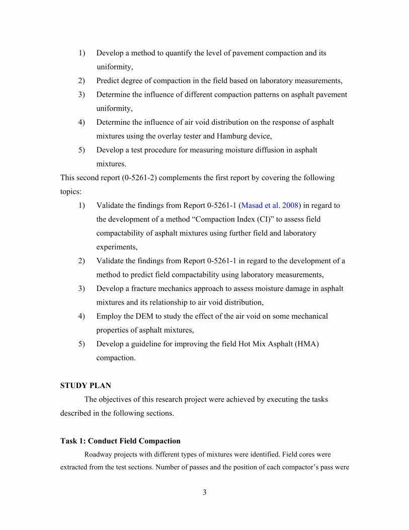
1) Develop a method to quantify the level of pavement compaction and its
uniformity,
2) Predict degree of compaction in the field based on laboratory measurements,
3) Determine the influence of different compaction patterns on asphalt pavement
uniformity,
4) Determine the influence of air void distribution on the response of asphalt
mixtures using the overlay tester and Hamburg device,
5) Develop a test procedure for measuring moisture diffusion in asphalt
mixtures.
This second report (0-5261-2) complements the first report by covering the following
topics:
1) Validate the findings from Report 0-5261-1 (Masad et al. 2008) in regard to
the development of a method “Compaction Index (CI)” to assess field
compactability of asphalt mixtures using further field and laboratory
experiments,
2) Validate the findings from Report 0-5261-1 in regard to the development of a
method to predict field compactability using laboratory measurements,
3) Develop a fracture mechanics approach to assess moisture damage in asphalt
mixtures and its relationship to air void distribution,
4) Employ the DEM to study the effect of the air void on some mechanical
properties of asphalt mixtures,
5) Develop a guideline for improving the field Hot Mix Asphalt (HMA)
compaction.
STUDY PLAN
The objectives of this research project were achieved by executing the tasks
described in the following sections.
Task 1: Conduct Field Compaction
Roadway projects with different types of mixtures were identified. Field cores were
extracted from the test sections. Number of passes and the position of each compactor’s pass were

4
recorded across the mat, and their influence on measured percent air voids in the recovered field
cores was studied. The data and samples collected during the field projects include:
• ambient, surface, and mixture temperature;
• density data measured using nuclear and non-nuclear density gauges;
• equipment used in the project, (screed, dump truck, or materials transfer device,
roller): size, weight, pattern, sequence, number of passes, etc.;
• cores for Saturated Surface Dry (SSD) density, vacuum sealed density, X-ray CT,
and performance testing; and
• plant mixture and virgin aggregate and binder for further testing.
Task 2: Analyze Air Void Distribution
X-ray Computed Tomography (CT) was used to capture the internal structure of
asphalt mixtures. The CT images were analyzed using image analysis techniques (Image-
Pro® Plus software 1999). Three-dimensional maps of air void distribution in pavement
sections were generated by inputting percent air voids as a function of depth (from X-ray
CT images) and the location of cores in the pavement to the Matlab 7.1 software (2004).
This application is considered valuable because it provides an estimate of percent air
voids at any point in the pavement section every 1 mm of depth. As such, one can
determine the detailed three-dimensional distribution of air voids. The uniformity of air
void distribution was quantified using mathematical indices.
Task 3: Evaluate Field Compactability and Laboratory Compactability
In the field, the location of the compactors across the mat during the compaction
process was recorded for each pass by measuring the distance from the edge of the
compactor with respect to the longitudinal joint of the mat. The compactability of asphalt
mixtures in the field was evaluated by considering the number of passes of the rollers and
the relative location of each pass. In the laboratory, a number of laboratory Superpave
Gyratory Compactor (SGC) specimens were compacted for the same asphalt mixtures
studied in the field. The compactability of the laboratory mixtures was quantified by
determining the slope of the percent air voids to number of gyrations on a logarithmic
scale for each sample at a certain percent air voids. The compactability of asphalt
5
mixtures in the laboratory was compared to the compaction index (CI) which quantifies
the compactability of the same mixtures in the field.
Task 4: Use Fracture Mechanics Approach to Assess Moisture Damage
The effect of air voids in asphalt mixtures on moisture susceptibility was
evaluated using a fracture mechanics approach that accounts for fundamental material
properties. Asphalt mixture samples with different percent air voids were prepared. Test
samples were subjected to dynamic loading under two different conditions: dry
(unconditioned) and wet (moisture-conditioned). The crack growth index developed by
Lytton et al. (1993) and later modified by Masad et al. (2006b) and Arambula (2007) was
employed in order to assess moisture susceptibility of asphalt mixtures. The parameters
required for the crack growth index were obtained through a relaxation modulus test, a
tensile test, a dynamic tensile test, and surface energy tests.
Task 5: Use DEM to Study Effect of Air Void on Mechanical Properties of Asphalt
Mixtures
This task focused on studying the air void effect on the Young’s modulus of
asphalt mixtures using Discrete Element Models (DEM). In this task, laboratory
specimens and field cores were scanned using X-ray CT to obtain the microstructure of
the air void levels. Two-dimensional and three-dimensional DEM models were
developed to evaluate the performance of the mixtures.
Task 6: Develop Guideline for Improving Field Compaction
Researchers submitted recommendations based on the findings of this study in
order to compact more uniform asphalt mixtures in the field and to assess the
compactability of asphalt mixtures in the field based on laboratory measurements. The
findings of the compactability of asphalt mixtures would be useful in achieving the
desired compaction levels in the field.
ORGANIZATION OF REPORT
This report documents the research efforts outlined in Tasks 1 through 6. Chapter
1 presents the overview, problem statement, objectives, and the list of tasks conducted
6
under this research project. Chapter 2 provides a brief description of the field projects,
field testing conducted in later part of the research project, and analyses of the uniformity
of air void distribution and the compactability of asphalt mixtures. Chapter 3 discusses
the fracture mechanics approach and the experimental tests used to assess the moisture
damage of asphalt mixtures with different percent of air voids. Chapter 4 reports the
efforts for studying the air void effect on the behavior of asphalt mixtures using DEM.
Chapter 5 introduces a brief guideline for improving the compaction of HMA mixture in
the field and decreasing the effort required to achieve desired field compaction. Finally,
Chapter 6 presents the overall conclusions and recommendations.

7
CHAPTER 2
EVALUATION OF FIELD COMPACTION
INTRODUCTION
As part of Task 2 and 3 outlined in Chapter 1, the research team identified and
conducted testing as part of 14 field HMA compaction projects in Texas. The first report
published from this project documented the research efforts and their findings from the
first 11 projects. This chapter documents the findings from the last three field projects
that were conducted in 2008.
DESCRIPTION OF TEST SECTIONS
Test sections from three field projects were evaluated with the help of the
TxDOT. These test sections were part of SH 44 in the Laredo District, SH 6 in the Bryan
District, and SL 1 (Mopac Highway) in the Austin District. The compaction pattern was
not modified from the one established by the contactor in these construction projects. The
researchers recorded field compaction effort; conducted tests in the field; obtained field
cores, plant mix, and virgin materials; and conducted laboratory tests on laboratory
compacted specimens and field cores. These test sections were studied to evaluate the
findings reported in Report 0-5261-1 (Masad et al. 2008). Table 2-1 provides a brief
description of mixtures used in these field projects; Table 2-2 summarizes the compaction
patterns. The following paragraphs briefly describe the research efforts and construction
projects included in this report.
SH 6 in Bryan District
This construction site was located south of Hearne in Robertson County in the
Bryan District. The test was conducted on the southbound outside lane in June 2008.
Both sides of the HMA mat were restrained. The contractor, Knife River Corporation,
placed 2-inch thick Stone Matrix Asphalt (SMA) after milling off the existing layer.
Before placement of SMA they applied tack coat. This SMA mixture was designed using
sandstone, limestone, and mineral filler with 6.4 percent PG 76-22 binder. This SMA
layer was again covered with one layer of seal coat and PFC. The research team
8
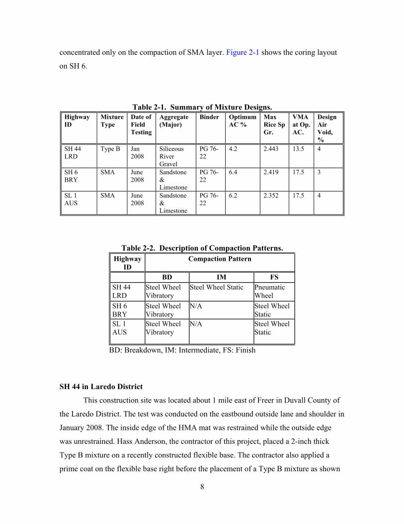
concentrated only on the compaction of SMA layer. Figure 2-1 shows the coring layout
on SH 6.
Table 2-1. Summary of Mixture Designs. Highway ID
Mixture Type
Date of Field Testing
Aggregate (Major)
Binder Optimum AC %
Max Rice Sp Gr.
VMA at Op. AC.
Design Air Void, %
SH 44 LRD
Type B Jan 2008
Siliceous River Gravel
PG 76-22
4.2 2.443 13.5 4
SH 6 BRY
SMA June 2008
Sandstone & Limestone
PG 76-22
6.4 2.419 17.5 3
SL 1 AUS
SMA June 2008
Sandstone & Limestone
PG 76-22
6.2 2.352 17.5 4
Table 2-2. Description of Compaction Patterns. Highway
ID Compaction Pattern
BD IM FS SH 44 LRD
Steel Wheel Vibratory
Steel Wheel Static Pneumatic Wheel
SH 6 BRY
Steel Wheel Vibratory
N/A Steel Wheel Static
SL 1 AUS
Steel Wheel Vibratory
N/A Steel Wheel Static
BD: Breakdown, IM: Intermediate, FS: Finish SH 44 in Laredo District
This construction site was located about 1 mile east of Freer in Duvall County of
the Laredo District. The test was conducted on the eastbound outside lane and shoulder in
January 2008. The inside edge of the HMA mat was restrained while the outside edge
was unrestrained. Hass Anderson, the contractor of this project, placed a 2-inch thick
Type B mixture on a recently constructed flexible base. The contractor also applied a
prime coat on the flexible base right before the placement of a Type B mixture as shown

9
in Figure 2-2. Finally one course seal coat layer was placed on the HMA surface as a
final surface. The research team was focused only on the compaction of the HMA layer.
This Type B mixture included primarily crushed river gravel with a 4.2 percent PG 76-22
binder.
Figure 2-1. Coring Layout on SH 6.
SL 1 in Austin District
This construction site was located in the City of Austin in the Austin District. It
was an SMA overlay project. The test was conducted on the southbound outside lane in
June 2008. Both sides of the HMA mat were restrained. Earlier the existing surface layer
was milled off, followed by placement of a one-layer seal coat. Due to high traffic
volume, the entire paving of this project was completed at night. This SMA mixture was
designed using sandstone, limestone, fly ash, and limestone screening with 6.2 percent
PG 76-22 binder.

10
Figure 2-2. Application of Prime Coat on Flexible Base.
RELATIONSHIP BETWEEN COMPACTION EFFORT AND PERCENT AIR
VOIDS
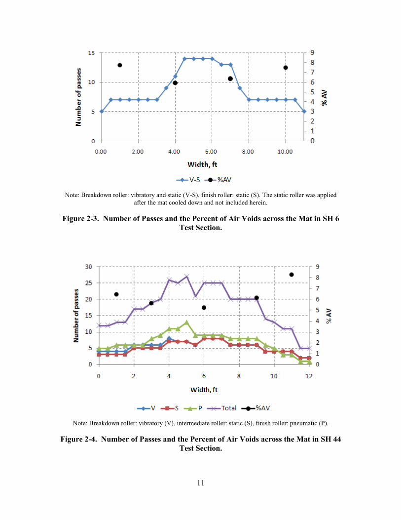
In each of the field projects, the research team recorded the number of roller
passes and their relative locations during each pass. Field cores were obtained from
different locations of the paving mat (white circles in Figure 2-1). The percent air voids
of the extracted field cores were measured using the Saturated Surface Dry (SSD)
Procedure (AASHTO 2002a). The number of passes of each compaction roller was
plotted along with the percent air voids across the test section. The percent air voids
represents the average percent of air voids of at least two cores taken longitudinally at a
given distance from the pavement section edge. Figures 2-3 through 2-5 show the results
of the test sections.
11
Note: Breakdown roller: vibratory and static (V-S), finish roller: static (S). The static roller was applied
after the mat cooled down and not included herein.
Figure 2-3. Number of Passes and the Percent of Air Voids across the Mat in SH 6 Test Section.
Note: Breakdown roller: vibratory (V), intermediate roller: static (S), finish roller: pneumatic (P).
Figure 2-4. Number of Passes and the Percent of Air Voids across the Mat in SH 44
Test Section.
12
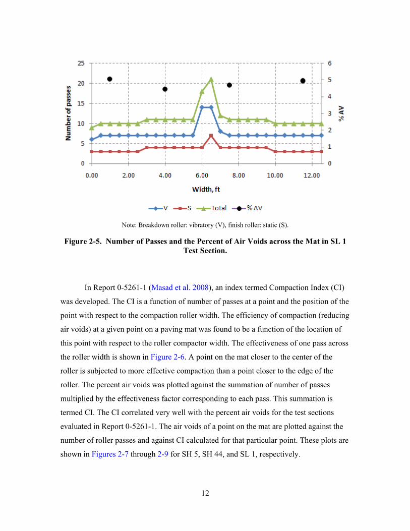
Note: Breakdown roller: vibratory (V), finish roller: static (S).
Figure 2-5. Number of Passes and the Percent of Air Voids across the Mat in SL 1
Test Section.
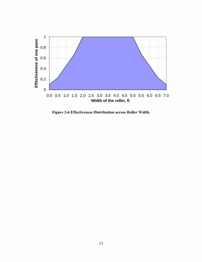
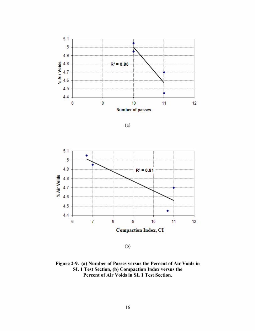
In Report 0-5261-1 (Masad et al. 2008), an index termed Compaction Index (CI)
was developed. The CI is a function of number of passes at a point and the position of the
point with respect to the compaction roller width. The efficiency of compaction (reducing
air voids) at a given point on a paving mat was found to be a function of the location of
this point with respect to the roller compactor width. The effectiveness of one pass across
the roller width is shown in Figure 2-6. A point on the mat closer to the center of the
roller is subjected to more effective compaction than a point closer to the edge of the
roller. The percent air voids was plotted against the summation of number of passes
multiplied by the effectiveness factor corresponding to each pass. This summation is
termed CI. The CI correlated very well with the percent air voids for the test sections
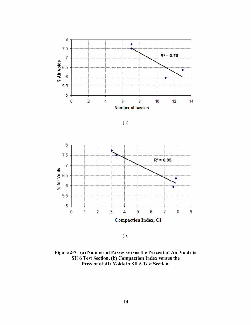
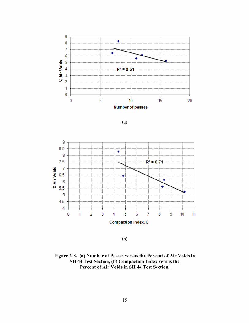
evaluated in Report 0-5261-1. The air voids of a point on the mat are plotted against the
number of roller passes and against CI calculated for that particular point. These plots are
shown in Figures 2-7 through 2-9 for SH 5, SH 44, and SL 1, respectively.
13
Figure 2-6 Effectiveness Distribution across Roller Width.
0
0.2
0.4
0.6
0.8
1
0.0 0.5 1.0 1.5 2.0 2.5 3.0 3.5 4.0 4.5 5.0 5.5 6.0 6.5 7.0
Effe
ctiv
enes
s of
one
pas
s
Width of the roller, ft
14
(a)
(b)
Figure 2-7. (a) Number of Passes versus the Percent of Air Voids in SH 6 Test Section, (b) Compaction Index versus the
Percent of Air Voids in SH 6 Test Section.
15
(a)
(b)
Figure 2-8. (a) Number of Passes versus the Percent of Air Voids in SH 44 Test Section, (b) Compaction Index versus the
Percent of Air Voids in SH 44 Test Section.
16
(a)
(b)
Figure 2-9. (a) Number of Passes versus the Percent of Air Voids in SL 1 Test Section, (b) Compaction Index versus the
Percent of Air Voids in SL 1 Test Section.
17
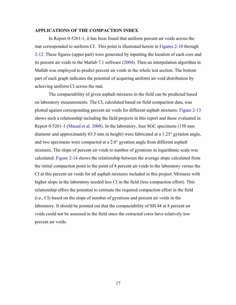
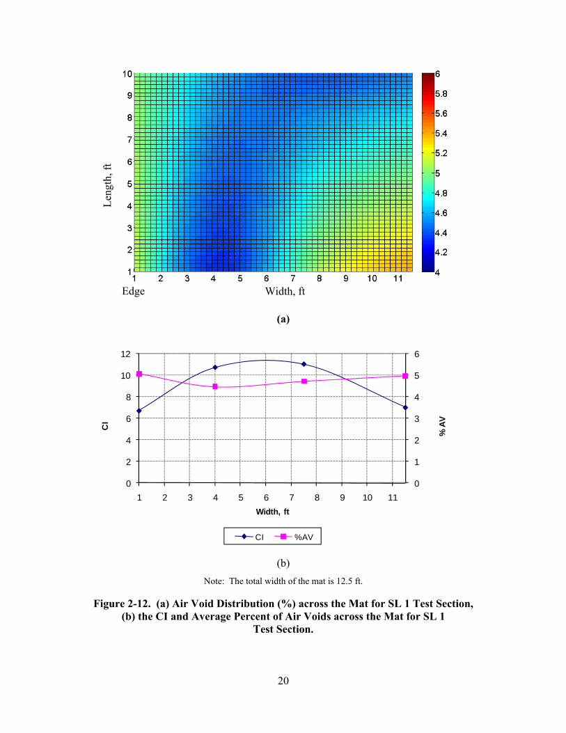
APPLICATIONS OF THE COMPACTION INDEX
In Report 0-5261-1, it has been found that uniform percent air voids across the
mat corresponded to uniform CI. This point is illustrated herein in Figures 2-10 through
2-12. These figures (upper part) were generated by inputting the location of each core and
its percent air voids to the Matlab 7.1 software (2004). Then an interpolation algorithm in
Matlab was employed to predict percent air voids in the whole test section. The bottom
part of each graph indicates the potential of acquiring uniform air void distribution by
achieving uniform CI across the mat.
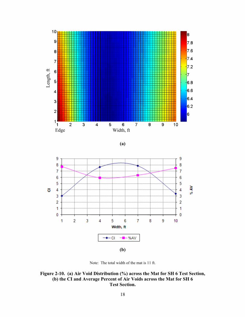
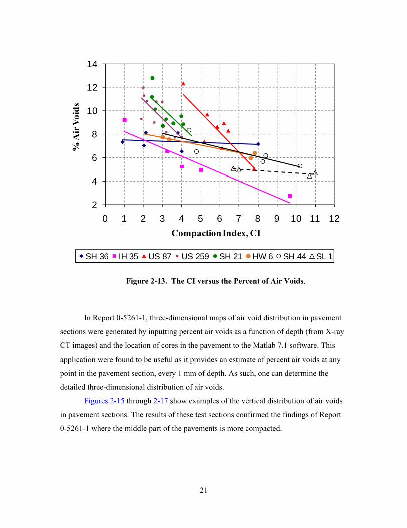
The compactability of given asphalt mixtures in the field can be predicted based
on laboratory measurements. The CI, calculated based on field compaction data, was
plotted against corresponding percent air voids for different asphalt mixtures. Figure 2-13
shows such a relationship including the field projects in this report and those evaluated in
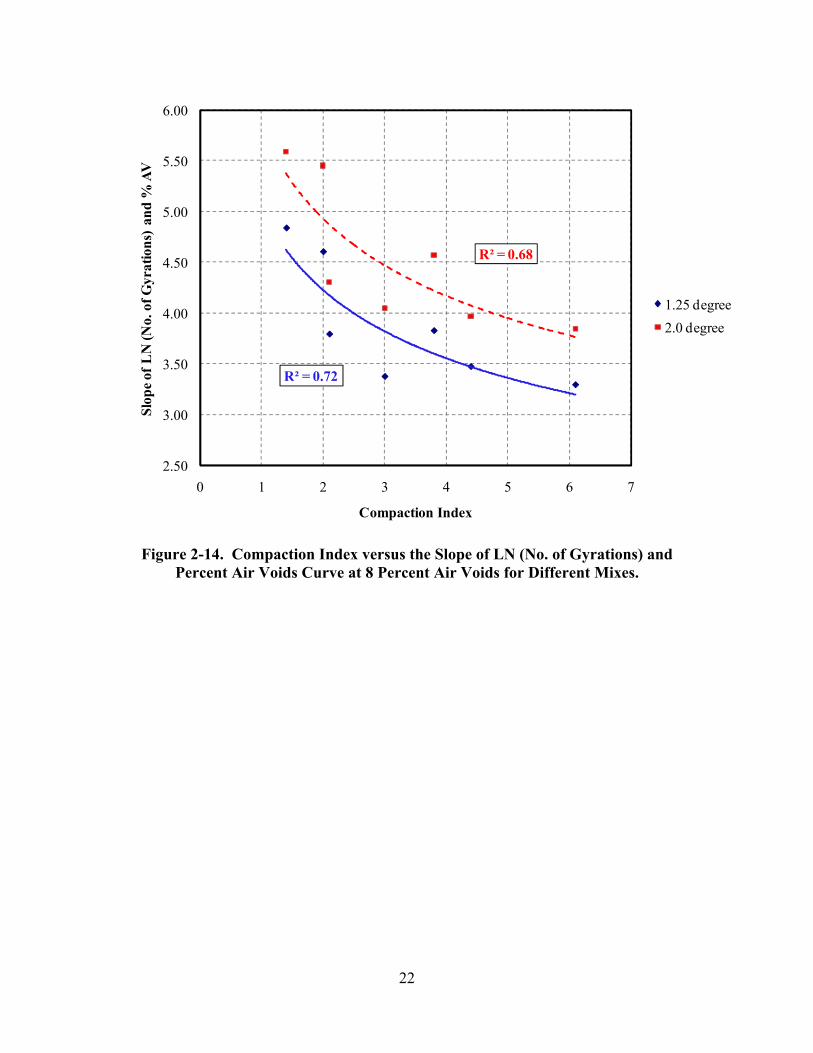
Report 0-5261-1 (Masad et al. 2008). In the laboratory, four SGC specimens (150 mm
diameter and approximately 63.5 mm in height) were fabricated at a 1.25° gyration angle,
and two specimens were compacted at a 2.0° gyration angle from different asphalt
mixtures. The slope of percent air voids to number of gyrations in logarithmic scale was
calculated. Figure 2-14 shows the relationship between the average slope calculated from
the initial compaction point to the point of 8 percent air voids in the laboratory versus the
CI at this percent air voids for all asphalt mixtures included in this project. Mixtures with
higher slope in the laboratory needed less CI in the field (less compaction effort). This
relationship offers the potential to estimate the required compaction effort in the field
(i.e., CI) based on the slope of number of gyrations and percent air voids in the
laboratory. It should be pointed out that the compactability of SH 44 at 8 percent air
voids could not be assessed in the field since the extracted cores have relatively low
percent air voids.
18
(a)
(b)
Note: The total width of the mat is 11 ft.
Figure 2-10. (a) Air Void Distribution (%) across the Mat for SH 6 Test Section,
(b) the CI and Average Percent of Air Voids across the Mat for SH 6 Test Section.
Leng
th, f
t
Width, ft Edge

19
(a)
(b)
Note: The total width of the mat is 12.0 ft.
Figure 2-11. (a) Air Void Distribution (%) across the Mat for SH 44 Test Section, (b) the CI and Average Percent of Air Voids across the Mat for SH 44
Test Section.
Leng
th, f
t
Width, ft Edge
20
(a)
(b)
Note: The total width of the mat is 12.5 ft.
Figure 2-12. (a) Air Void Distribution (%) across the Mat for SL 1 Test Section, (b) the CI and Average Percent of Air Voids across the Mat for SL 1
Test Section.
0
1
2
3
4
5
6
0
2
4
6
8
10
12
1 2 3 4 5 6 7 8 9 10 11
% A
V
CI
Width, ft
CI %AV
Leng
th, f
t
Width, ft Edge
21
Figure 2-13. The CI versus the Percent of Air Voids.
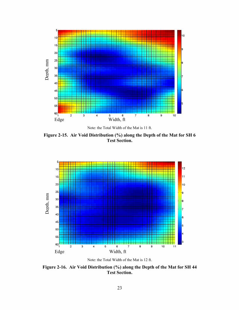
In Report 0-5261-1, three-dimensional maps of air void distribution in pavement
sections were generated by inputting percent air voids as a function of depth (from X-ray
CT images) and the location of cores in the pavement to the Matlab 7.1 software. This
application were found to be useful as it provides an estimate of percent air voids at any
point in the pavement section, every 1 mm of depth. As such, one can determine the
detailed three-dimensional distribution of air voids.
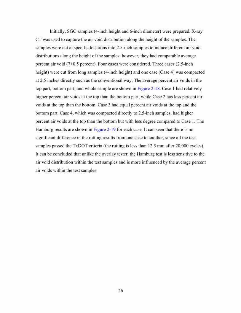
Figures 2-15 through 2-17 show examples of the vertical distribution of air voids
in pavement sections. The results of these test sections confirmed the findings of Report
0-5261-1 where the middle part of the pavements is more compacted.
2
4
6
8
10
12
14
0 1 2 3 4 5 6 7 8 9 10 11 12
% A
ir V
oids
Compaction Index, CI
SH 36 IH 35 US 87 US 259 SH 21 HW 6 SH 44 SL 1
22
Figure 2-14. Compaction Index versus the Slope of LN (No. of Gyrations) and
Percent Air Voids Curve at 8 Percent Air Voids for Different Mixes.
R² = 0.72
R² = 0.68
2.50
3.00
3.50
4.00
4.50
5.00
5.50
6.00
0 1 2 3 4 5 6 7
Slop
e of L
N (N
o. o
f Gyr
atio
ns)
and
% A
V
Compaction Index
1.25 degree2.0 degree
23
Note: the Total Width of the Mat is 11 ft.
Figure 2-15. Air Void Distribution (%) along the Depth of the Mat for SH 6 Test Section.
Note: the Total Width of the Mat is 12 ft.
Figure 2-16. Air Void Distribution (%) along the Depth of the Mat for SH 44 Test Section.
Width, ft Edge
Dep
th, m
m
Width, ft
Dep
th, m
m
Edge

24
Note: the Total Width of the Mat is 12.5 ft.
Figure 2-17. Air Void Distribution (%) along the Depth of the Mat for SL 1 Test Section.
Comparison of Laboratory and Field Mechanical Properties
The research team obtained field cores from the test sections. These cores were
tested to measure density, air void distribution using X-ray CT, permeability, rutting
resistance using a Hamburg wheel tracking device, and fatigue resistance using an
overlay tester. In addition, laboratory specimens were prepared using virgin materials
obtained from the HMA plants for the test projects. These tests procedures were
discussed in detail in Report 0-5261-1. Table 2-3 summarizes the results with the
specimens obtained from the last three field projects.
Dep
th, m
m
Width, ft Edge

25
Table 2-3. Summary of Mechanical Tests Results.
Permeability Test, Overlay Test, Hamburg Test,
cm/sec # of Cycles Rutting Rate
Field Lab. Field Lab. Field Lab.
HW 6 1.0x10⁻³ 1.0x10⁻³ 900+ 642 2.79 0.79
SH 44 5.83x10⁻⁴ 5.82x10⁻⁴ 88 105 0.55 0.49
SL 1 8.5x10⁻⁴ 1.3x10⁻³ 900+ 22 2.32 0.75
EFFECT OF THE AIR VOID DISTRIBUTION ON THE HAMBURG TEST
In Report 0-5261-1, the effect of air void distribution on the overlay test results
was evaluated. In this section, the effect of the air void distribution on the Hamburg test
results was evaluated. The Hamburg results were found to be influenced by the average
percent air void (Masad et al. 2008); however the effect of the air void distribution on the
Hamburg results was not easy to be evaluated for the following reasons:
• The field cores have a dissimilar percent of air voids which make it difficult to
correlate the Hamburg results with the air void structure without considering the
effect of the percent of air voids.
• The field cores, which have similar percent air voids, did not have the similar air
void distribution in all the projects in this study.
For the previous two reasons, it was difficult to acquire a comprehensive
conclusion for all the projects. In order to overcome this problem, a side study was
initiated to eliminate the dissimilarity of the percent of the air voids and the average air
void distribution. This study included testing a number of laboratory samples fabricated
in such a way to induce different air void distributions along the height of the samples.
These samples had 7 percent air voids ± 0.50 percent air voids. The US 259 mix,
described in Report 0-5261-1, was used in this study as it has experienced a considerable
amount of the rutting.
26
Initially, SGC samples (4-inch height and 6-inch diameter) were prepared. X-ray
CT was used to capture the air void distribution along the height of the samples. The
samples were cut at specific locations into 2.5-inch samples to induce different air void
distributions along the height of the samples; however, they had comparable average
percent air void (7±0.5 percent). Four cases were considered. Three cases (2.5-inch
height) were cut from long samples (4-inch height) and one case (Case 4) was compacted
at 2.5 inches directly such as the conventional way. The average percent air voids in the
top part, bottom part, and whole sample are shown in Figure 2-18. Case 1 had relatively
higher percent air voids at the top than the bottom part, while Case 2 has less percent air
voids at the top than the bottom. Case 3 had equal percent air voids at the top and the
bottom part. Case 4, which was compacted directly to 2.5-inch samples, had higher
percent air voids at the top than the bottom but with less degree compared to Case 1. The
Hamburg results are shown in Figure 2-19 for each case. It can seen that there is no
significant difference in the rutting results from one case to another, since all the test
samples passed the TxDOT criteria (the rutting is less than 12.5 mm after 20,000 cycles).
It can be concluded that unlike the overlay tester, the Hamburg test is less sensitive to the
air void distribution within the test samples and is more influenced by the average percent
air voids within the test samples.

27
Figure 2-18. The Average, Top, and Bottom Percent of Air Voids for Different
Cases.
Figure 2-19. Hamburg Test Results for Different Cases.
0
2
4
6
8
10
Case 1 Case 2 Case 3 Case 4
Perc
ent A
ir Vo
ids
Top Bottom Average
28
CONCLUSIONS
The results of the three test sections evaluated in this part of the project agreed
with the findings from Report 0-5261-1. The percent of air voids correlated well with the
compaction effort across the mat. The compaction effort was found to be a function of the
number of roller passes and the location of each pass across the mat. The efficiency of
compaction at a given point is a function of the location of this point with respect to the
roller width. A new index, referred to as the Compaction Index, is proposed to quantify
the compaction effort at any point in the pavement. The CI is used to study the
compactability of asphalt mixtures in the field. The CI correlated well with the slope of
the laboratory compaction curves. Asphalt mixtures with higher slope in laboratory
needed less CI in the field to achieve the same percent air void. In addition, it was found
that in most of the test sections the middle part (across the depth) of the mat is more
compacted than the top and bottom parts.

29
CHAPTER 3
FRACTURE-BASED ANALYSIS OF INFLUENCE OF AIR VOIDS
ON MOISTURE DAMAGE
INTRODUCTION AND OBJECTIVES
As discussed in Report 0-5261-1, percent and size of air voids is an important
factor that influences asphalt pavement performance. In this chapter, experimental
methods and a fracture mechanics approach that accounts for fundamental material
properties are used to evaluate the resistance of asphalt mixtures with different percent air
voids to moisture damage. Asphalt mixture specimens with different percent air voids
were prepared. Test specimens were subjected to dynamic loading under two different
conditions: dry (unconditioned) and wet (moisture-conditioned). The moisture
conditioning was conducted such that specimens with different percent air voids had the
same amount of moisture by varying the moisture conditioning time.
The crack growth index developed originally by Lytton (1993) and later modified
and implemented by Masad et al. (2006b) and Arambula (2007) was employed in order to
assess resistance to moisture damage. The inputs of the fracture model include the
viscoelastic properties, pseudostrain dissipated energy, tensile strength, and the adhesive
bond surface energy of asphalt mixture.
ASPHALT MIXTURES TEST SPECIMENS
This mixture was used in the construction of the overlay of the SH 87 in the
Yoakum District. The mixture was Type C (TxDOT 1993 Specifications) and designed
with Fordyce Gravel and Colorado Materials limestone screening with a PG 76-22
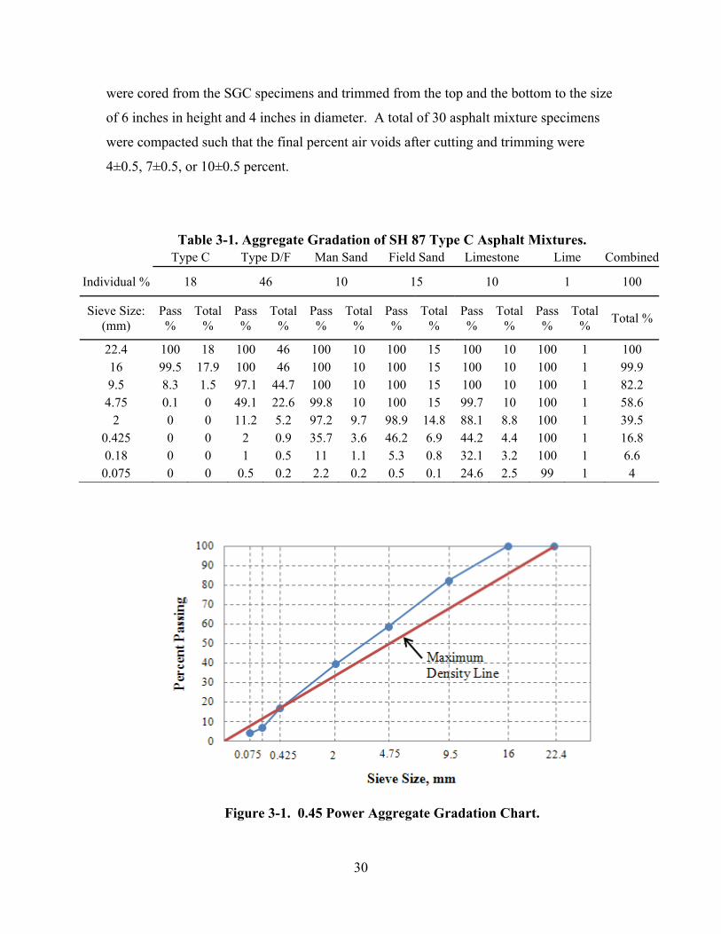
binder. The aggregate gradation is given in Table 3-1 and shown in Figure 3-1.
The Superpave gyratory compactor was used to compact laboratory cylindrical
asphalt mixture specimens. The specimens were prepared according to AASHTO
standards (2002b). The mixing and compaction temperatures were determined according
to TxDOT 2005 specifications based on the binder grade. The mixing and compaction
temperature for the PG 76-22s binder are 325oF and 300oF, respectively. The laboratory
SGC specimens were 7 inches in height and 6 inches in diameter. The test specimens
30
were cored from the SGC specimens and trimmed from the top and the bottom to the size
of 6 inches in height and 4 inches in diameter. A total of 30 asphalt mixture specimens
were compacted such that the final percent air voids after cutting and trimming were
4±0.5, 7±0.5, or 10±0.5 percent.
Table 3-1. Aggregate Gradation of SH 87 Type C Asphalt Mixtures. Type C Type D/F Man Sand Field Sand Limestone Lime Combined
Individual % 18 46 10 15 10 1 100
Sieve Size: (mm)
Pass %
Total %
Pass %
Total %
Pass %
Total %
Pass %
Total %
Pass %
Total %
Pass %
Total % Total %
22.4 100 18 100 46 100 10 100 15 100 10 100 1 100 16 99.5 17.9 100 46 100 10 100 15 100 10 100 1 99.9 9.5 8.3 1.5 97.1 44.7 100 10 100 15 100 10 100 1 82.2
4.75 0.1 0 49.1 22.6 99.8 10 100 15 99.7 10 100 1 58.6 2 0 0 11.2 5.2 97.2 9.7 98.9 14.8 88.1 8.8 100 1 39.5
0.425 0 0 2 0.9 35.7 3.6 46.2 6.9 44.2 4.4 100 1 16.8 0.18 0 0 1 0.5 11 1.1 5.3 0.8 32.1 3.2 100 1 6.6 0.075 0 0 0.5 0.2 2.2 0.2 0.5 0.1 24.6 2.5 99 1 4
Figure 3-1. 0.45 Power Aggregate Gradation Chart.

31
MOISTURE CONDITIONING
Half of the test specimens (five specimens at each percent air voids) were
subjected to moisture conditioning following the modified Lottman procedure without the
freezing stage (AASHTO 2007). A vacuum of 3.38 kPa absolute pressure (736.6 mm Hg.
partial pressure) was used in this study for moisture conditioning. Several specimens at
different percent air voids were prepared and conditioned for different times in order to
determine the time needed to achieve the required saturation level between 70 to 80
percent as required by AASHTO T-283-07. The time measurement started once a
vacuum of 3.38 kPa absolute pressure was achieved. Table 3-2 presents the time required
to achieve the target saturation level for specimens with different percent air voids. This
procedure was followed by placing specimens in a 60 oC water bath for 24 hours. Then,
the test specimens were taken to another 20 oC water bath to cool down before testing.
Table 3-2. Vacuum Saturation Time. Percent Time,
Air Voids Sec 4 90 7 45 10 25
EXPERIMENTAL TESTS
The following section will cover the experimental tests by which the model’s
inputs were determined.
Relaxation Test
This test was used to determine the viscoelastic properties which include the
initial relaxation modulus (Eo) and the modulus relaxation rate (m). A constant axial
tension strain of 80 microstrain was applied to the test specimens for 60 sec followed by
600 sec rest period. Then, a constant compression strain of 80 microstrain was applied for
60 sec. The time interval used to increase the load from 0 to a constant value of 80
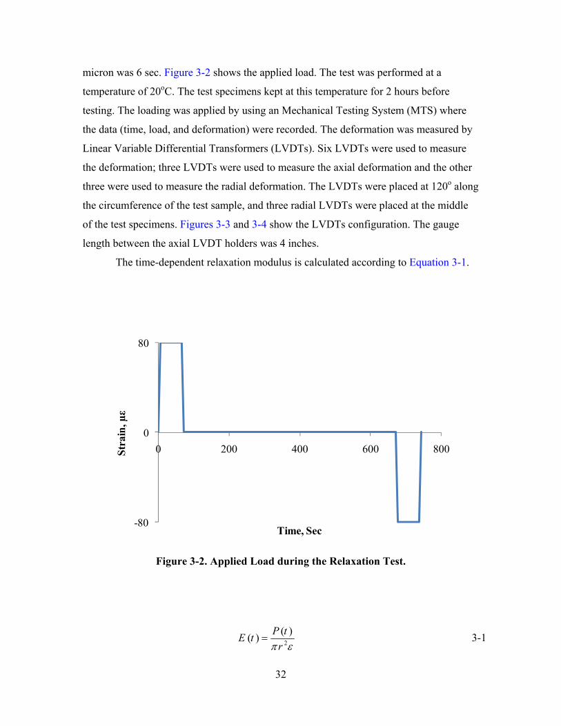
32
micron was 6 sec. Figure 3-2 shows the applied load. The test was performed at a
temperature of 20oC. The test specimens kept at this temperature for 2 hours before
testing. The loading was applied by using an Mechanical Testing System (MTS) where
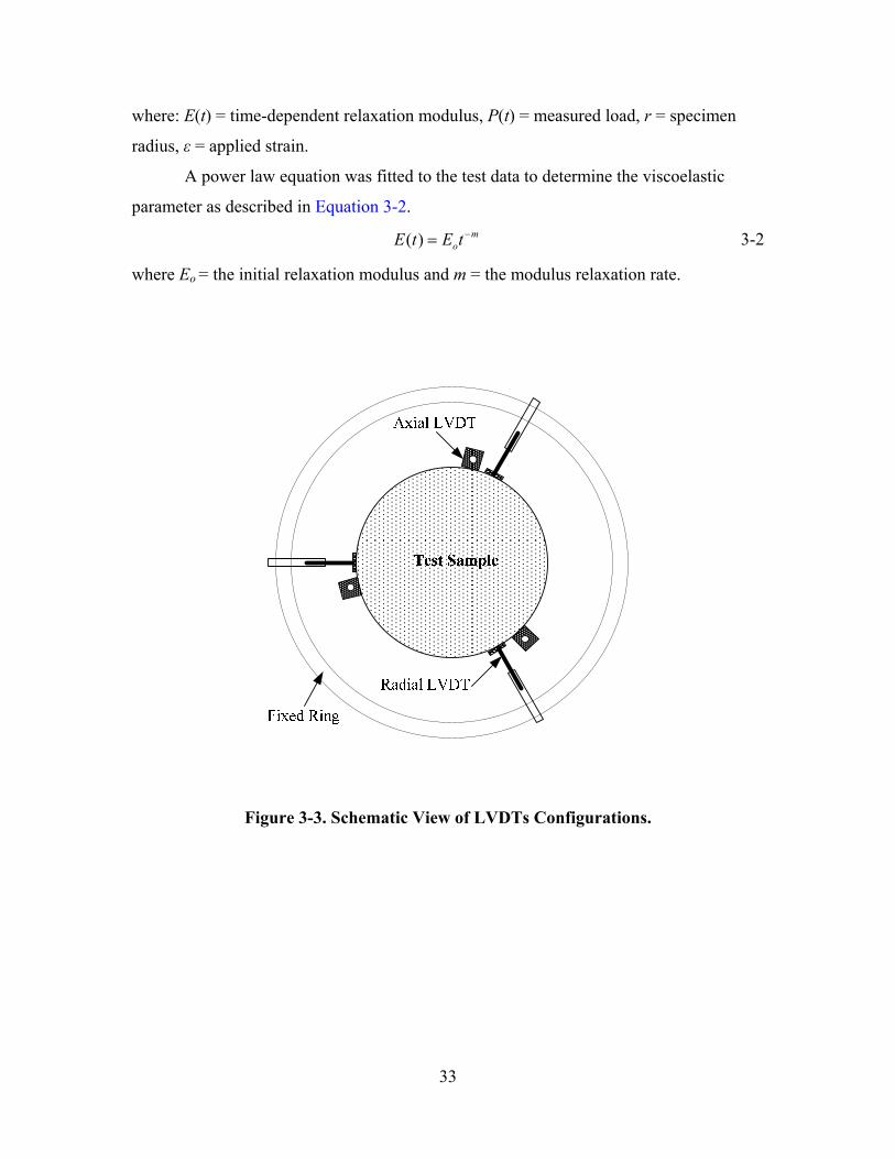
the data (time, load, and deformation) were recorded. The deformation was measured by
Linear Variable Differential Transformers (LVDTs). Six LVDTs were used to measure
the deformation; three LVDTs were used to measure the axial deformation and the other
three were used to measure the radial deformation. The LVDTs were placed at 120o along
the circumference of the test sample, and three radial LVDTs were placed at the middle
of the test specimens. Figures 3-3 and 3-4 show the LVDTs configuration. The gauge
length between the axial LVDT holders was 4 inches.
The time-dependent relaxation modulus is calculated according to Equation 3-1.
Figure 3-2. Applied Load during the Relaxation Test.
2
( )( ) P tE trπ ε
= 3-1
-80
0
80
0 200 400 600 800Stra
in, µε
Time, Sec
33
where: E(t) = time-dependent relaxation modulus, P(t) = measured load, r = specimen
radius, ε = applied strain.
A power law equation was fitted to the test data to determine the viscoelastic
parameter as described in Equation 3-2.
( ) moE t E t −= 3-2
where Eo = the initial relaxation modulus and m = the modulus relaxation rate.
Figure 3-3. Schematic View of LVDTs Configurations.
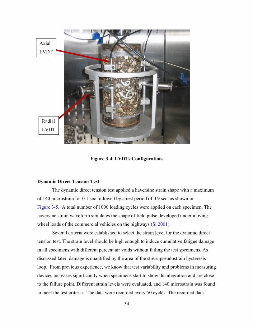
34
Figure 3-4. LVDTs Configuration.
Dynamic Direct Tension Test
The dynamic direct tension test applied a haversine strain shape with a maximum
of 140 microstrain for 0.1 sec followed by a rest period of 0.9 sec, as shown in
Figure 3-5. A total number of 1000 loading cycles were applied on each specimen. The
haversine strain waveform simulates the shape of field pulse developed under moving
wheel loads of the commercial vehicles on the highways (Si 2001).
Several criteria were established to select the strain level for the dynamic direct
tension test. The strain level should be high enough to induce cumulative fatigue damage
in all specimens with different percent air voids without failing the test specimens. As
discussed later, damage is quantified by the area of the stress-pseudostrain hysteresis
loop. From previous experience, we know that test variability and problems in measuring
devices increases significantly when specimens start to show disintegration and are close
to the failure point. Different strain levels were evaluated, and 140 microstrain was found
to meet the test criteria. The data were recorded every 50 cycles. The recorded data
Radial
LVDT
Axial
LVDT

35
points within a single loading cycle should be sufficient to study the dissipated
pseudostrain energy. In this test, for every single recorded loading cycle, the data were
captured every 0.005 sec. The LVDTs configurations were the exact same used in the
relaxation modulus test. The test was conducted at a constant temperature of 20oC. Test
specimens were conditioned at this temperature for about two hours before conducting
the test.
Figure 3-5 Applied Loading Configurations for Dynamic Direct Tension Test.
The viscoelastic stress ( Vσ ) was computed using the Boltzman superposition for
every loading cycle as follows (Arambula 2007):
1
( ) ( )k
mV k o k i i
i
E t C dtσ τ τ −
=
= −∑ 3-3
where: Eo = initial relaxation modulus determined using the relaxation test, τk and ti = the
present and previous time, m = the modulus relaxation rate determined using the
relaxation test, Ci = (dε/dt) the change in strain for every load increment, dt = time
increment, k = number of data points.
0
140
0 1 2 3
Stra
in, µε
Number of Cycles
1000

36
The measured time-dependent tensile stress was calculated in Equation 3-4.
2
( )( )mP tt
rσ
π= 3-4
where: P(t) = the measured load, r = the radius of the sample.
The reference modulus (ER) was estimated according to Equation 3-5.
( ) max( ) max
mR
tEt
σε
= 3-5
where: σm(t)max = the maximum measured time-dependent tensile stress at the first load
cycle, ε(t)max = the maximum measured time-dependent tensile strain at the
corresponding cycle.
The pseudostrain (εR) is the ratio between the viscoelastic stress ( Vσ ) and the
reference modulus (ER) as given in Equation 3-6.
( )( ) VR
R
ttE
σε = 3-6
The dissipated pseudostrain energy (DPSE) is the area of hysteresis loop of the measured
tensile stress ( )m tσ against the calculated pseudostrain (εR) as shown in Figure 3-6. The
area was computed using the double meridian distance method (Wolf and Ghilani 2002).
To account for the reduction in the matter that is able to dissipate the energy, the DPSE
was normalized by the ratio of (PSi/PSo) as follows:
( / )R
i o
DPSEWPS PS
= 3-7
where, WR= normalized DPSE, PSi = pseudostiffness at each load cycle, and PSo = the
maximum pseudostiffness at the first load cycle. The pseudostiffness is the ratio of
maximum measured stress to maximum computed pseudostrain. The normalized DPSE
quantifies the real damage during the dynamic direct tension test.
The relationship between the normalized DPSE (WR) and the number of load
cycles is presented in a semi-log graph in Figure 3-7. This relationship yields a trend line
which has the following form:
ln( )RW a b N= + 3-8
where, b = the rate of fracture damage accumulation, a = the energy associated with the
initial damage which corresponds to the first load cycle.

37
Figure 3-6 An Example of Measured Stress vs. Pseudostrain.
Figure 3-7. Normalized DPSE, WR vs. Number of Cycles.
-40
-20
0
20
40
60
80
100
120
-5.0E-05 0.0E+00 5.0E-05 1.0E-04 1.5E-04
Mea
sure
d St
ress
, Psi
Pseudostrain (in/in)

38
Tensile Strength Test
This test was used to determine the tensile strength of the test specimens. The
tensile strength is a required input in the fracture model. This test was conducted at 20oC
after 10 min of the completion of the dynamic direct tension test. A test sample was
continuously pulled at a constant rate of 0.05 inch/min until the failure occurs.
Figure 3-8 shows a test specimen after failure inside the Materials Testing System
(MTS), while Figure 3-9 shows the failure for the test specimens in dry and wet
conditions. Figure 3-9(a) displays the failure in wet condition where the aggregates were
stripped from the binder. Figure 3-9(b) shows the failure in dry condition where the
aggregates were still coated very well with the binder.
Figure 3-8. Test Sample after Failure inside the MTS.

39
(a) (b)
Figure 3-9. Test Specimens after Failure (a) Wet Condition, (b) Dry Condition. Surface Energy Measurements
The surface energy was used to estimate the adhesive bond surface energy
between asphalt binder and aggregate and the cohesive bond energy of asphalt binder
(Arambula 2007; Howson et al. 2007). The surface energy can be defined as the required
work to create a unit surface area. The surface free energy has three separate components
(Howson et al. 2007): monopolar acidic (Γ+,), monopolar basic (Γ-) and apolar or
Lifshitz-van der Waals (ΓLW). The total surface free energy is calculated according to
Equation 3-9.
2LW + −Γ = Γ + Γ Γ 3-9
The adhesive bond energy (ΔGf) is a required parameter in the proposed model.
The Wilhelmy plate (WP) test and the Universal sorption device (USD) are used to
determine the surface energy components of asphalt binder and aggregates, respectively.
Table 3-3 presents the surface energy components for the asphalt binder and aggregates.
The adhesive bond energy between the binder (subscript A) and aggregate
(subscript S) was calculated using Equation 3-10. The adhesive bond energy when the
water (subscript W) displaces asphalt binder from its interface with the aggregate is
presented in Equation 3-11.
2 2 2a LW LWAS A S A S A SG + − − +Δ = Γ Γ + Γ Γ + Γ Γ 3-10
wetASW AW SW ASGΔ = Γ +Γ −Γ 3-11
40
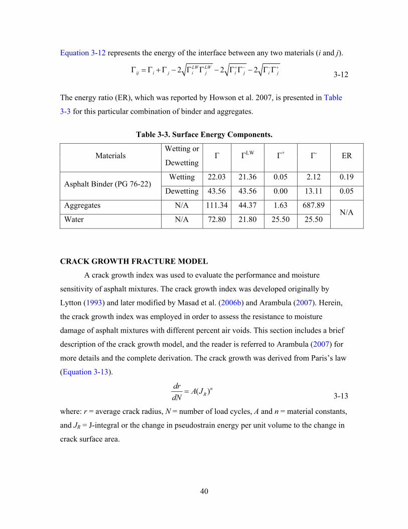
Equation 3-12 represents the energy of the interface between any two materials (i and j).
2 2 2LW LWij i j i j i j i j
+ − − +Γ = Γ +Γ − Γ Γ − Γ Γ − Γ Γ 3-12
The energy ratio (ER), which was reported by Howson et al. 2007, is presented in Table
3-3 for this particular combination of binder and aggregates.
Table 3-3. Surface Energy Components.
Materials Wetting or
Γ ΓLW Γ+ Γ- ER Dewetting
Asphalt Binder (PG 76-22) Wetting 22.03 21.36 0.05 2.12 0.19
Dewetting 43.56 43.56 0.00 13.11 0.05
Aggregates N/A 111.34 44.37 1.63 687.89 N/A
Water N/A 72.80 21.80 25.50 25.50
CRACK GROWTH FRACTURE MODEL
A crack growth index was used to evaluate the performance and moisture
sensitivity of asphalt mixtures. The crack growth index was developed originally by
Lytton (1993) and later modified by Masad et al. (2006b) and Arambula (2007). Herein,
the crack growth index was employed in order to assess the resistance to moisture
damage of asphalt mixtures with different percent air voids. This section includes a brief
description of the crack growth model, and the reader is referred to Arambula (2007) for
more details and the complete derivation. The crack growth was derived from Paris’s law
(Equation 3-13).
( )nR
dr A JdN
= 3-13
where: r = average crack radius, N = number of load cycles, A and n = material constants,
and JR = J-integral or the change in pseudostrain energy per unit volume to the change in
crack surface area.
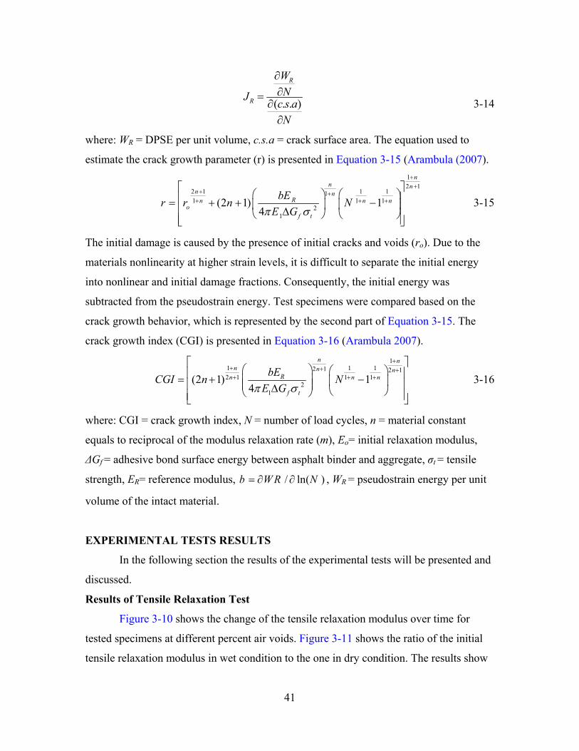
41
( . . )
R
R
WNJ c s aN
∂∂=
∂∂
3-14
where: WR = DPSE per unit volume, c.s.a = crack surface area. The equation used to
estimate the crack growth parameter (r) is presented in Equation 3-15 (Arambula (2007).
12 1
2 1 1 111 1 1
21
(2 1) 14
nn n
n nRn n n
of t
bEr r n NE Gπ σ
++
+ ++ + +
⎡ ⎤⎛ ⎞⎛ ⎞⎢ ⎥= + + −⎜ ⎟⎜ ⎟⎢ ⎥Δ⎝ ⎠ ⎝ ⎠⎢ ⎥⎣ ⎦
3-15
The initial damage is caused by the presence of initial cracks and voids (ro). Due to the
materials nonlinearity at higher strain levels, it is difficult to separate the initial energy
into nonlinear and initial damage fractions. Consequently, the initial energy was
subtracted from the pseudostrain energy. Test specimens were compared based on the
crack growth behavior, which is represented by the second part of Equation 3-15. The
crack growth index (CGI) is presented in Equation 3-16 (Arambula 2007).
11 1 12 1 2 12 1 1 1
21
(2 1) 14
n nn n n
Rn n n
f t
bECGI n NE Gπ σ
++ + ++ + +
⎡ ⎤⎛ ⎞ ⎛ ⎞⎢ ⎥= + −⎜ ⎟ ⎜ ⎟⎢ ⎥⎜ ⎟Δ ⎝ ⎠⎝ ⎠⎢ ⎥⎣ ⎦
3-16
where: CGI = crack growth index, N = number of load cycles, n = material constant
equals to reciprocal of the modulus relaxation rate (m), Eo= initial relaxation modulus,
ΔGf = adhesive bond surface energy between asphalt binder and aggregate, σt = tensile
strength, ER= reference modulus, / ln( )b W R N= ∂ ∂ , WR = pseudostrain energy per unit
volume of the intact material.
EXPERIMENTAL TESTS RESULTS
In the following section the results of the experimental tests will be presented and
discussed.
Results of Tensile Relaxation Test
Figure 3-10 shows the change of the tensile relaxation modulus over time for
tested specimens at different percent air voids. Figure 3-11 shows the ratio of the initial
tensile relaxation modulus in wet condition to the one in dry condition. The results show
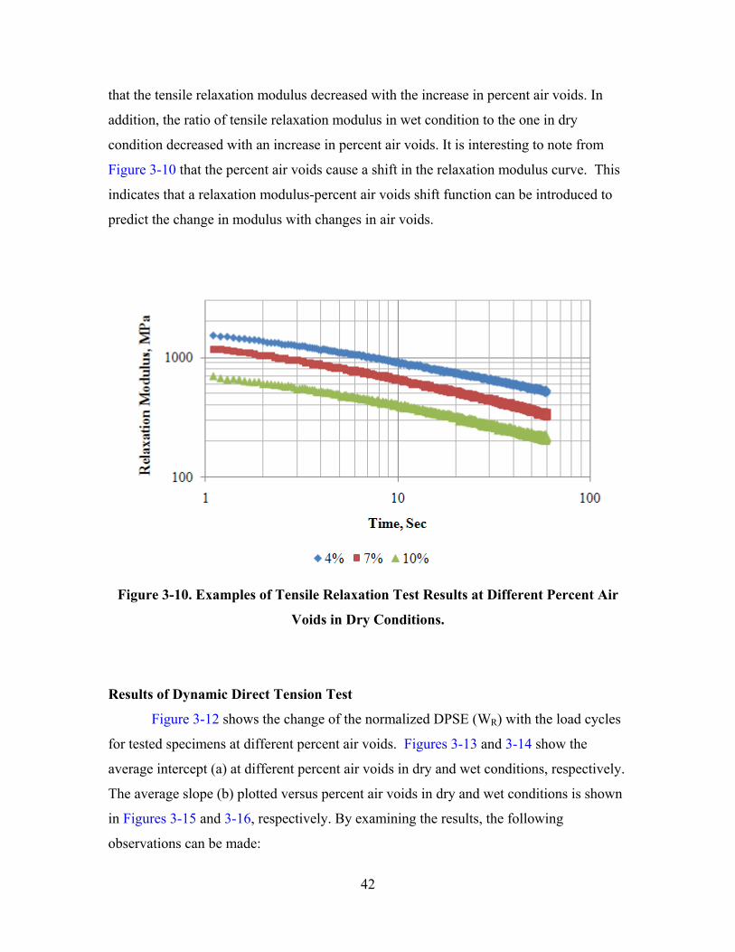
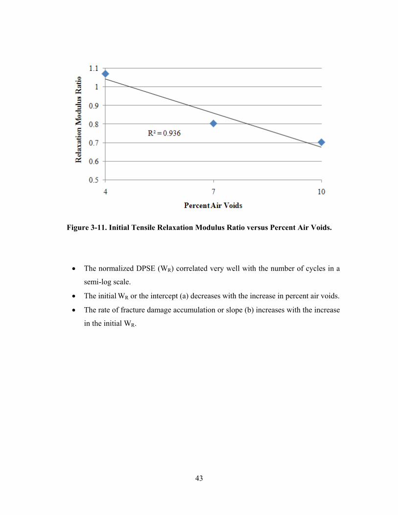
42
that the tensile relaxation modulus decreased with the increase in percent air voids. In
addition, the ratio of tensile relaxation modulus in wet condition to the one in dry
condition decreased with an increase in percent air voids. It is interesting to note from
Figure 3-10 that the percent air voids cause a shift in the relaxation modulus curve. This
indicates that a relaxation modulus-percent air voids shift function can be introduced to
predict the change in modulus with changes in air voids.
Figure 3-10. Examples of Tensile Relaxation Test Results at Different Percent Air
Voids in Dry Conditions.
Results of Dynamic Direct Tension Test
Figure 3-12 shows the change of the normalized DPSE (WR) with the load cycles
for tested specimens at different percent air voids. Figures 3-13 and 3-14 show the
average intercept (a) at different percent air voids in dry and wet conditions, respectively.
The average slope (b) plotted versus percent air voids in dry and wet conditions is shown
in Figures 3-15 and 3-16, respectively. By examining the results, the following
observations can be made:
43
Figure 3-11. Initial Tensile Relaxation Modulus Ratio versus Percent Air Voids.
• The normalized DPSE (WR) correlated very well with the number of cycles in a
semi-log scale.
• The initial WR or the intercept (a) decreases with the increase in percent air voids.
• The rate of fracture damage accumulation or slope (b) increases with the increase
in the initial WR.

44
Figure 3-12. Normalized DPSE (WR) versus Number of Cycles at Different Percent
Air Voids.
Figure 3-13. Intercept (a) versus Percent Air Voids in Dry Conditions.

45
Figure 3-14. Intercept (a) versus Percent Air Voids in Wet Conditions.
Figure 3-15. Percent Air Voids versus Slope (b) in Dry Conditions.

46
Figure 3-16. Percent Air Voids versus Slope (b) in Wet Conditions.
Results of Tensile Strength Test
Figures 3-17 and 3-18 present the average tensile strength for test specimens with
different percent air voids in dry and wet conditions, respectively. The ratio of the
average tensile strength in wet condition to the average tensile strength in dry condition at
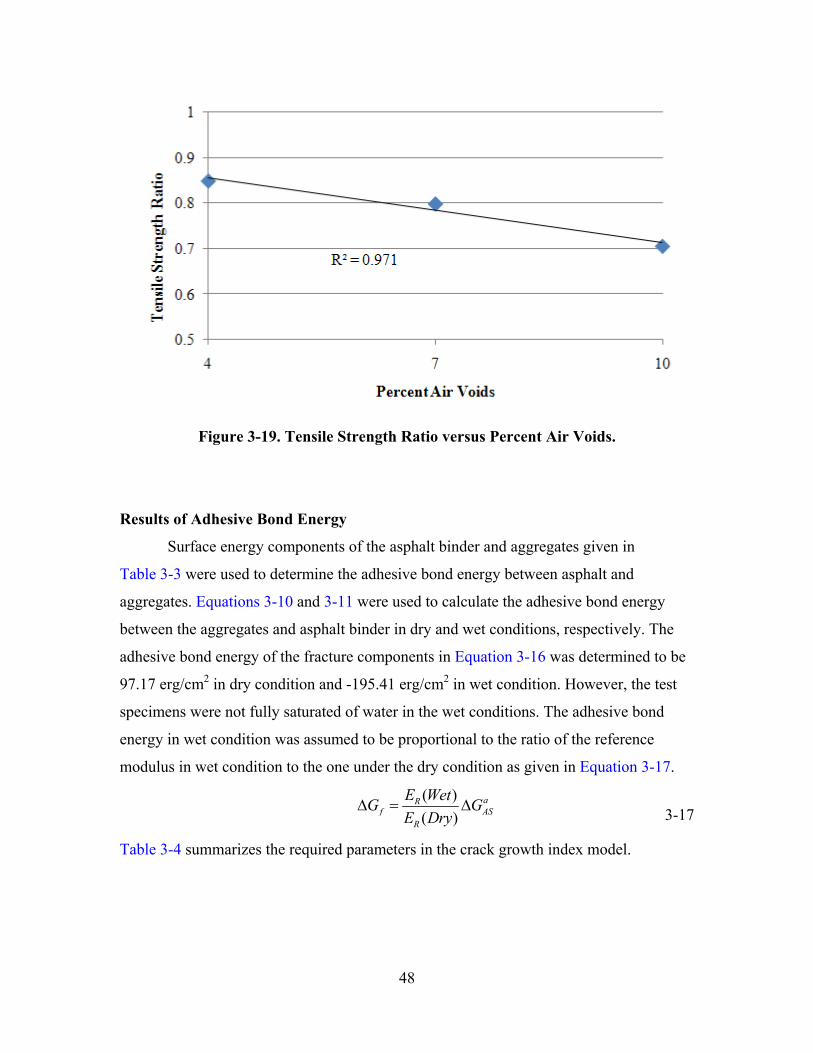
different percent air voids is shown in Figure 3-19. The results show the following:
• The tensile strength decreased with the increase in percent air voids.
• The ratio of tensile strength in wet condition to the one in dry condition
decreased with the increase in percent air voids.

47
Figure 3-17 Average Tensile Strength versus Percent Air Voids in Dry Conditions.
Figure 3-18. Average Tensile Strength versus Percent Air Voids in Wet Conditions.
48
Figure 3-19. Tensile Strength Ratio versus Percent Air Voids.
Results of Adhesive Bond Energy
Surface energy components of the asphalt binder and aggregates given in
Table 3-3 were used to determine the adhesive bond energy between asphalt and
aggregates. Equations 3-10 and 3-11 were used to calculate the adhesive bond energy
between the aggregates and asphalt binder in dry and wet conditions, respectively. The
adhesive bond energy of the fracture components in Equation 3-16 was determined to be
97.17 erg/cm2 in dry condition and -195.41 erg/cm2 in wet condition. However, the test
specimens were not fully saturated of water in the wet conditions. The adhesive bond
energy in wet condition was assumed to be proportional to the ratio of the reference
modulus in wet condition to the one under the dry condition as given in Equation 3-17.
( )( )
aRf AS
R
E WetG GE Dry
Δ = Δ 3-17
Table 3-4 summarizes the required parameters in the crack growth index model.
49
Table 3-4. Average Parameters for the Fracture Model. Percent
Condition E0
m ER a
b σt ΔGf
Air Voids Mpa Mpa J/m3 kPa J/m2
4
Dry 1843.38 0.316 5469.36 25.97 2.45 1100.69 0.09717
Wet 1974.2 0.341 5375.76 24.35 2.46 935.17 0.09551
7
Dry 1394.34 0.318 4437.34 21.43 2.03 816.55 0.09717
Wet 1122.37 0.334 3983.1 19.56 1.44 652.41 0.08722
10
Dry 808.05 0.298 4094.03 12.79 1.03 594.48 0.09717
Wet 594.38 0.316 3436.79 10.09 0.65 419.31 0.08456
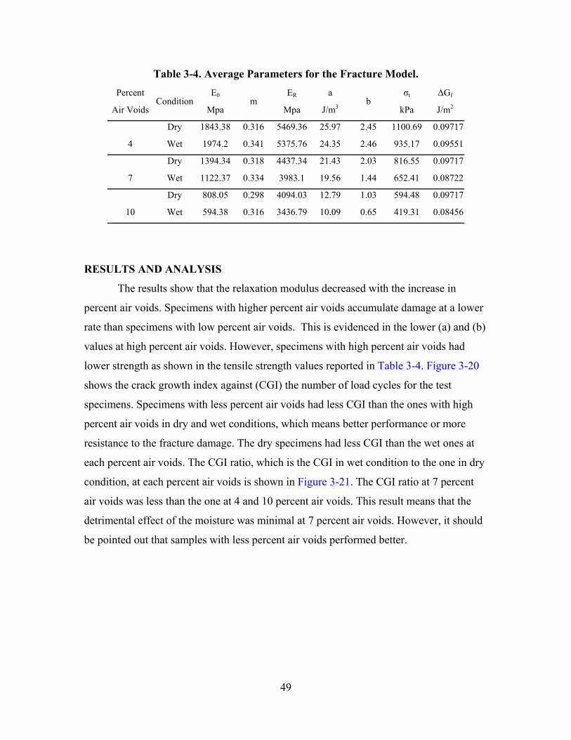
RESULTS AND ANALYSIS
The results show that the relaxation modulus decreased with the increase in
percent air voids. Specimens with higher percent air voids accumulate damage at a lower
rate than specimens with low percent air voids. This is evidenced in the lower (a) and (b)
values at high percent air voids. However, specimens with high percent air voids had
lower strength as shown in the tensile strength values reported in Table 3-4. Figure 3-20
shows the crack growth index against (CGI) the number of load cycles for the test
specimens. Specimens with less percent air voids had less CGI than the ones with high
percent air voids in dry and wet conditions, which means better performance or more
resistance to the fracture damage. The dry specimens had less CGI than the wet ones at
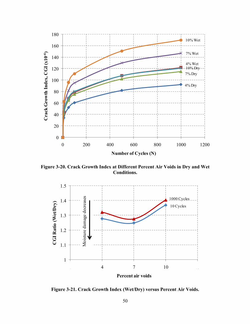
each percent air voids. The CGI ratio, which is the CGI in wet condition to the one in dry
condition, at each percent air voids is shown in Figure 3-21. The CGI ratio at 7 percent
air voids was less than the one at 4 and 10 percent air voids. This result means that the
detrimental effect of the moisture was minimal at 7 percent air voids. However, it should
be pointed out that samples with less percent air voids performed better.
50
Figure 3-20. Crack Growth Index at Different Percent Air Voids in Dry and Wet
Conditions.
Figure 3-21. Crack Growth Index (Wet/Dry) versus Percent Air Voids.
0
20
40
60
80
100
120
140
160
180
0 200 400 600 800 1000 1200
Cra
ck G
row
th In
dex,
CG
I (x1
0-6)
Number of Cycles (N)
7% Dry10% Dry4% Wet
7% Wet
10% Wet
4% Dry
1
1.1
1.2
1.3
1.4
1.5
1 4 7 10 13
CG
I Rat
io (W
et/D
ry)
Percent air voids
10 Cycles
1000 Cycles
Moi
stur
e da
mag
e de
crea
ses
51
SUMMARY
In this chapter, the resistance of asphalt mixtures with different percent air voids
to moisture damage was evaluated by using a fracture mechanics approach. This
approach accounts for fundamental material properties which include the viscoelastic
properties, pseudostrain dissipated energy, tensile strength, and the adhesive bond surface
energy of asphalt mixture. Dry and wet test asphalt mixtures specimens were evaluated.
A crack growth index was used to quantify the damage of the test specimens. The dry
samples performed better than the wet ones at each percent air voids. The test specimens
with less percent air voids performed better than the ones with higher percent air voids.
The detrimental effect of moisture at 7 percent air voids specimens was the least
compared to 4 and 10 percent air voids specimens.
The crack growth fracture model clearly demonstrates the effect of different
percent air voids on the performance of asphalt mixtures. In addition, the model shows
that the detrimental effect of moisture was the greatest at a higher percent air voids, 10
percent. These results show the importance of compaction level on the performance of
asphalt mixtures. Effective compaction results in less percent air voids and provides
better performance. In addition, the fracture mechanics approach presented in this chapter
is a valuable method to evaluate different asphalt mixture designs and select the one with
good resistance to moisture damage.

52
53
CHAPTER 4
DISCRETE ELEMENT MODELS OF MECHANICAL PROPERTIES
OF ASPHALT MIXTURES* INTRODUCTION
Air voids play an important role in the performance of asphalt mixtures as seen in
Chapter 3. This chapter focuses on investigating the air void effect of the mechanical
properties of the asphalt mixtures using Discrete Element Models (DEM). Laboratory
samples and field cores were evaluated. Test specimens were scanned using X-ray CT to
obtain the images of the microstructure of the air void levels. In the simulation of
mechanical properties of the asphalt, two-dimensional (2D) and three-dimensional (3D)
discrete element models were prepared to evaluate the performance of the mixtures. In
the 2D models, both vertical- and horizontal-cut images of the 3D specimen were used to
evaluate the different air void levels. In addition, the relationship between the mixture
modulus versus the air void levels was investigated.
SCOPE
This study focuses on the effects of different air void levels on asphalt mixtures.
The application of the DEM approach was limited to the uniaxial, biaxial, and triaxial
compression test. The 2D and 3D microstructures of the asphalt mixture were obtained
with the X-ray CT technique. The DEM models were based upon the microstructures of
the mixtures.
BACKGROUND OF MICROMECHANICAL MODELS
The micromechanical modeling technique has been successfully used in the past
decade. A unified theory for predicting the overall behavior of composite materials was
_________________
*Reprinted with the permission from “Microstructural and Micromechanical Properties of Field and Lab-Compacted Asphalt Mixtures” by You, Z., Adhikari, S., Masad, E., and Dai, Q., 2009, Journal of the Association of Asphalt Paving Technologists, AAPT, Vol. (78).

54
proposed to analyze the mechanical behavior of the materials (Aboudi 1991; Aboudi
2004). The cell method was used to predict the strength and fatigue failure of composite
materials. A basis for research activity on the micromechanics of heterogeneous materials
was provided by Nemat-Nasser and Hori (1999).
Most current micromechanical models for the asphalt mixture have been used to
predict asphalt mixture’s mechanical properties based upon the ingredients (Li et al. 1999;
Papagiannakis et al. 2002). Based upon progress of the other researchers, a microstructure-
based finite element model for the asphalt mixture (a heterogeneous material) was
developed (Dai et al. 2006; Dai and You 2006). Multiphase asphalt mixture materials,
including aggregates and mastic, were divided into different subdomains. The complex
modulus of the mixture was then predicted by compression tests (Dai and You 2006). The
comparison between the finite element model prediction and laboratory measurement
indicated that the predictions were reliable for the asphalt mixtures.
The Discrete Element Method was applied to the particle flow of granular
materials. The granular medium is represented by an assembly of discrete blocks which
can be considered as rigid or deformable. The method is based on the formulation and
solution of the equations of motion or deformation of these discrete blocks and the
contacts between them. The contact must be identified by proper constitutive models
during the entire deformation or motion process. This study involves the use of a
commercially available discrete element program called Particle Flow Code (PFC) in
Two Dimensions or PFC2D (Itasca 2004a) and Three Dimensions or PFC3D (Itasca
2004b).
Buttlar and You (2001) proposed a microfabric approach to model asphalt
mixture using the discrete element methods, where various material phases (i.e.,
aggregates and mastic) in the asphalt mixture were modeled with bonded clusters of 2D
discrete elements. You et al. (2008) predicted the asphalt mixture modulus across a range
of temperatures and loading frequencies using 3D discrete element models.
TEST SPECIMENS AND X-RAY CT
Three SGC laboratory specimens and eight field cores were evaluated in this
study. The laboratory specimens are 6.5 inches (165 mm) in height by 6 inches (150 mm)
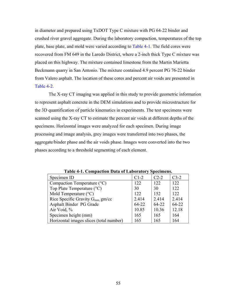
55
in diameter and prepared using TxDOT Type C mixture with PG 64-22 binder and
crushed river gravel aggregate. During the laboratory compaction, temperatures of the top
plate, base plate, and mold were varied according to Table 4-1. The field cores were
recovered from FM 649 in the Laredo District, where a 2-inch thick Type C mixture was
placed on this highway. The mixture contained limestone from the Martin Marietta
Beckmann quarry in San Antonio. The mixture contained 4.9 percent PG 76-22 binder
from Valero asphalt. The location of these cores and percent air voids are presented in
Table 4-2.
The X-ray CT imaging was applied in this study to provide geometric information
to represent asphalt concrete in the DEM simulations and to provide microstructure for
the 3D quantification of particle kinematics in experiments. The test specimens were
scanned using the X-ray CT to estimate the percent air voids at different depths of the
specimens. Horizontal images were analyzed for each specimen. During image
processing and image analysis, grey images were transferred into two phases, the
aggregate/binder phase and the air voids phase. Images were converted into the two
phases according to a threshold segmenting of each element.
Table 4-1. Compaction Data of Laboratory Specimens. Specimen ID C1-2 C2-2 C3-2 Compaction Temperature (°C) 122 122 122 Top Plate Temperature (°C) 30 30 122 Mold Temperature (°C) 122 152 122 Rice Specific Gravity Gmm, gm/cc 2.414 2.414 2.414 Asphalt Binder PG Grade 64-22 64-22 64-22 Air Void, % 10.85 10.36 12.18 Specimen height (mm) 165 165 164 Horizontal images slices (total number) 165 165 164
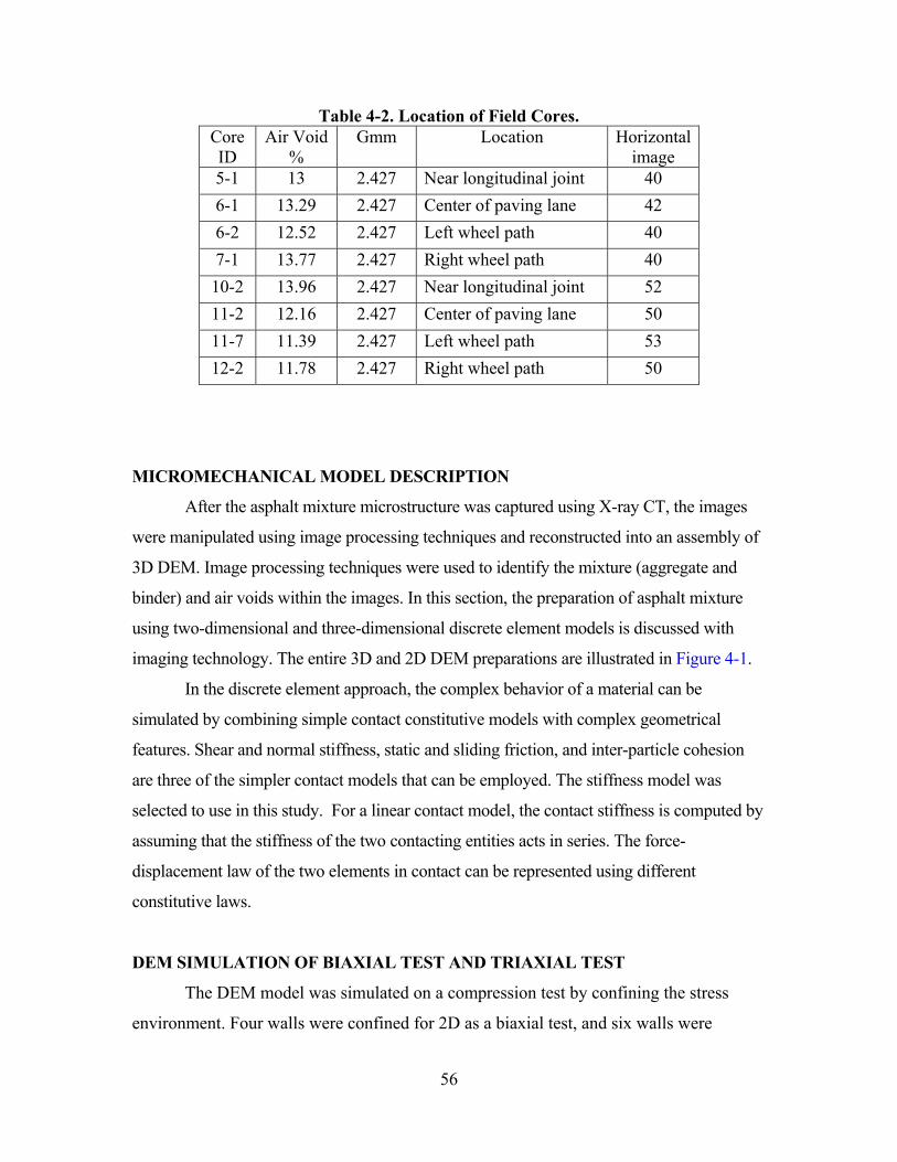
56
Table 4-2. Location of Field Cores. Core ID
Air Void %
Gmm Location Horizontal image
5-1 13 2.427 Near longitudinal joint 40 6-1 13.29 2.427 Center of paving lane 42 6-2 12.52 2.427 Left wheel path 40 7-1 13.77 2.427 Right wheel path 40 10-2 13.96 2.427 Near longitudinal joint 52 11-2 12.16 2.427 Center of paving lane 50 11-7 11.39 2.427 Left wheel path 53 12-2 11.78 2.427 Right wheel path 50
MICROMECHANICAL MODEL DESCRIPTION
After the asphalt mixture microstructure was captured using X-ray CT, the images
were manipulated using image processing techniques and reconstructed into an assembly of
3D DEM. Image processing techniques were used to identify the mixture (aggregate and
binder) and air voids within the images. In this section, the preparation of asphalt mixture
using two-dimensional and three-dimensional discrete element models is discussed with
imaging technology. The entire 3D and 2D DEM preparations are illustrated in Figure 4-1.
In the discrete element approach, the complex behavior of a material can be
simulated by combining simple contact constitutive models with complex geometrical
features. Shear and normal stiffness, static and sliding friction, and inter-particle cohesion
are three of the simpler contact models that can be employed. The stiffness model was
selected to use in this study. For a linear contact model, the contact stiffness is computed by
assuming that the stiffness of the two contacting entities acts in series. The force-
displacement law of the two elements in contact can be represented using different
constitutive laws.
DEM SIMULATION OF BIAXIAL TEST AND TRIAXIAL TEST
The DEM model was simulated on a compression test by confining the stress
environment. Four walls were confined for 2D as a biaxial test, and six walls were
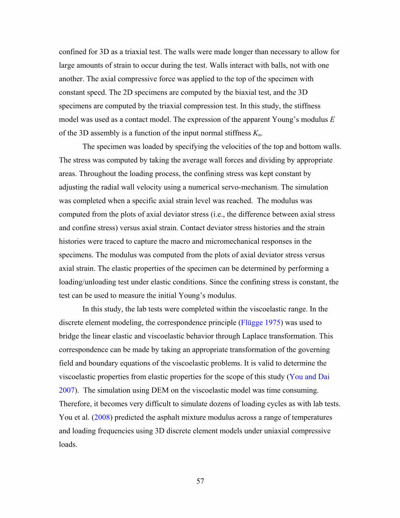
57
confined for 3D as a triaxial test. The walls were made longer than necessary to allow for
large amounts of strain to occur during the test. Walls interact with balls, not with one
another. The axial compressive force was applied to the top of the specimen with
constant speed. The 2D specimens are computed by the biaxial test, and the 3D
specimens are computed by the triaxial compression test. In this study, the stiffness
model was used as a contact model. The expression of the apparent Young’s modulus E
of the 3D assembly is a function of the input normal stiffness Kn.
The specimen was loaded by specifying the velocities of the top and bottom walls.
The stress was computed by taking the average wall forces and dividing by appropriate
areas. Throughout the loading process, the confining stress was kept constant by
adjusting the radial wall velocity using a numerical servo-mechanism. The simulation
was completed when a specific axial strain level was reached. The modulus was
computed from the plots of axial deviator stress (i.e., the difference between axial stress
and confine stress) versus axial strain. Contact deviator stress histories and the strain
histories were traced to capture the macro and micromechanical responses in the
specimens. The modulus was computed from the plots of axial deviator stress versus
axial strain. The elastic properties of the specimen can be determined by performing a
loading/unloading test under elastic conditions. Since the confining stress is constant, the
test can be used to measure the initial Young’s modulus.
In this study, the lab tests were completed within the viscoelastic range. In the
discrete element modeling, the correspondence principle (Flügge 1975) was used to
bridge the linear elastic and viscoelastic behavior through Laplace transformation. This
correspondence can be made by taking an appropriate transformation of the governing
field and boundary equations of the viscoelastic problems. It is valid to determine the
viscoelastic properties from elastic properties for the scope of this study (You and Dai
2007). The simulation using DEM on the viscoelastic model was time consuming.
Therefore, it becomes very difficult to simulate dozens of loading cycles as with lab tests.
You et al. (2008) predicted the asphalt mixture modulus across a range of temperatures
and loading frequencies using 3D discrete element models under uniaxial compressive
loads.
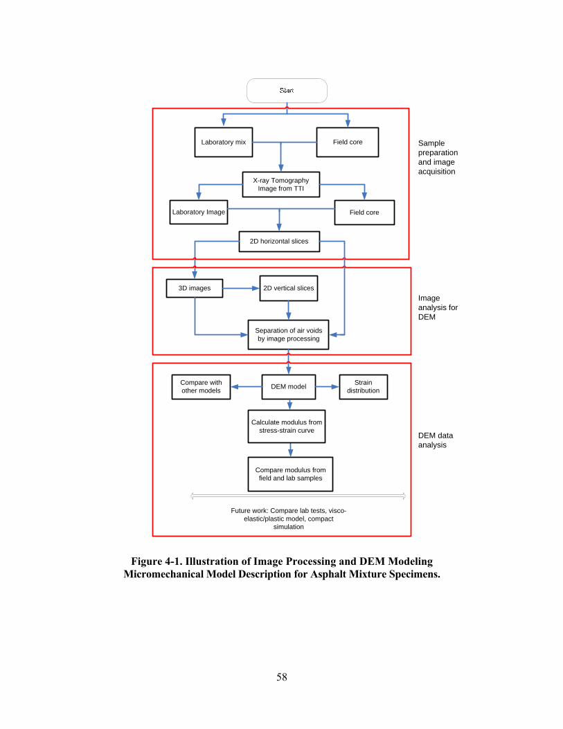
58
Laboratory mix Field core
X-ray Tomography Image from TTI
2D horizontal slices
2D vertical slices
Separation of air voids by image processing
DEM model Strain distribution
Compare modulus from field and lab samples
Future work: Compare lab tests, visco-elastic/plastic model, compact
simulation
Laboratory Image Field core
Compare with other models
Calculate modulus from stress-strain curve
3D images
Sample preparation and image acquisition
Image analysis for DEM
DEM data analysis
Figure 4-1. Illustration of Image Processing and DEM Modeling Micromechanical Model Description for Asphalt Mixture Specimens.

59
MICROSTRUCTURE RECONSTRUCTION
In order to examine the stiffness of the asphalt mixture, 2D and 3D discrete element
models were used to predict the mixture moduli of the asphalt mixture at different air voids
levels. The 3D model was composed of a number of 2D discrete element layers. Both 2D
and 3D models were generated using regular packing balls/spheres. The 2D DEM was
generated from the vertical and horizontal orientation of the 3D cylinder-shaped specimen
as shown in Figure 4-2.
b) 2D Vertical Orientation
c) 2D Horizontal Orientation
Figure 4-2. Vertical and Horizontal “Cut” of the X-ray Images for the 2D Vertical and Horizontal Models.
a) 3D Model X1 X2
X3
X4
X5
Y1, Y2, Y3, Y4, Y5
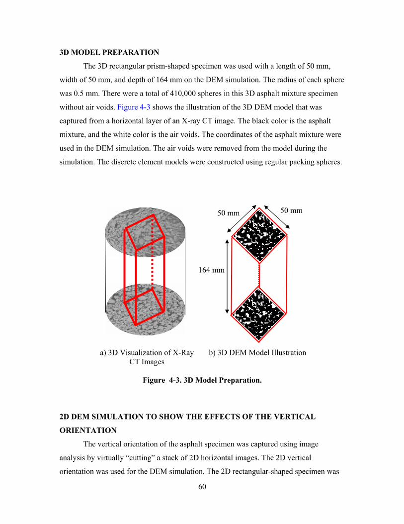
60
3D MODEL PREPARATION
The 3D rectangular prism-shaped specimen was used with a length of 50 mm,
width of 50 mm, and depth of 164 mm on the DEM simulation. The radius of each sphere
was 0.5 mm. There were a total of 410,000 spheres in this 3D asphalt mixture specimen
without air voids. Figure 4-3 shows the illustration of the 3D DEM model that was
captured from a horizontal layer of an X-ray CT image. The black color is the asphalt
mixture, and the white color is the air voids. The coordinates of the asphalt mixture were
used in the DEM simulation. The air voids were removed from the model during the
simulation. The discrete element models were constructed using regular packing spheres.
a) 3D Visualization of X-Ray CT Images
b) 3D DEM Model Illustration
Figure 4-3. 3D Model Preparation.
2D DEM SIMULATION TO SHOW THE EFFECTS OF THE VERTICAL
ORIENTATION
The vertical orientation of the asphalt specimen was captured using image
analysis by virtually “cutting” a stack of 2D horizontal images. The 2D vertical
orientation was used for the DEM simulation. The 2D rectangular-shaped specimen was
50 mm 50 mm
164 mm

61
generated having a height of 512 units (or 150 mm) and a width of 512 units (or 150 mm)
from the images. The radius of each ball (discrete element) was 0.5 unit (0.15 mm).
There were a total of 262,144 balls in the digital or virtual specimen. The vertical
orientation of the 3D specimen is 71 mm, 73 mm, 75 mm, 77 mm, and 79 mm from the
surface of the specimen. There were a total of 15 vertical slices from the 3 specimens.
The air voids of the vertical images were calculated using Matlab software. Figure 4-4
shows the 2D air void distribution in the DEM in different replicates of 3D specimens for
which the measurements are compared. The inner 2D sections have lower air voids than
the outer sections. The modulus of the vertical orientation of the specimen was predicted
using DEM simulation. Figure 4-5 shows the normalized modulus of the vertical
orientation. The modulus of an asphalt mixture is considered to be unity in the absence
of any air void. In other words, when there is no existence of air void, the matrix of the
model is in fact a one-phase model, and the modulus of the model should be 1.0 when the
input is 1.0. When the air void exists, the modulus of the model becomes less than 1.0
when the modulus of the matrix is 1. In the following sections, the normalized modulus is
provided for all the 2D and 3D models in order to study the air void effects.
2D DEM SIMULATION TO SHOW THE EFFECTS OF THE HORIZONTAL
ORIENTATION
The horizontal orientation of the asphalt specimen was obtained from horizontal
slices of X-ray CT images. The total of 18 horizontal images was used for DEM
simulation using 3 specimens. The horizontal orientation is obtained by “cutting” the
specimen at height 15 mm, 50 mm, 75 mm, 100 mm, 125 mm, and 150 mm from the top
surface of the specimen to the bottom. These 2D horizontal images were used for DEM
simulation. The 2D rectangular shaped specimen was generated with the height of 50 mm
and width of 50 mm from the images. The radius of each ball (discrete element) was 0.5
mm. The air voids of the horizontal images are calculated using Matlab software. Figure
4-6 shows the calculated and measured air voids of the horizontal orientation. As seen
from the figure, the air void levels are different depending on the locations of the “cut”.
The top and bottom 2D sections have higher air voids than the middle sections. The
modulus of the vertical orientation of the specimen was predicted using DEM simulation.

62
Figure 4-7 shows the modulus prediction of the 2D horizontal orientation of
corresponding air void levels. It shows that the lower the air voids, the higher the moduli,
and vice versa.
Figure 4-4. Air Void of the Vertical Section of the Three Specimens (2D Models).
Figure 4-5. Normalized Modulus of the Vertical Section of Three Specimens (2D
Models).
02468
101214
C1-2 C2-2 C3-2Laboratoy specimens
Air
Void
, %
71 73 75 77 79 Measurement
Position
00.1
0.20.3
0.40.5
0.60.7
C1-2 C2-2 C3-2Laboratoy specimens
Nor
mal
ized
mod
ulus
71 73 75 77 79
Position
Laboratory Specimens
Laboratory Specimens
Air
Void
, %
Nor
mal
ized
Mod
ulus

63
Figure 4-6. Air Void of the Horizontal Section of the Specimens.
Figure 4-7. Normalized Modulus of the Horizontal Section of the Specimens (2D Models).
COMPARE 3D MODELS, 2D VERTICAL ORIENTATION MODELS, AND 2D
HORIZONTAL ORIENTATION MODELS
Compressive test simulations were conducted using the 2D and 3D discrete
element models. The modulus of the asphalt mixture was predicted as described before.
In this section, the 2D and 3D discrete element models are discussed to compare whether
0
5
10
15
20
C1-2 C2-2 C3-2Laboratoy specimens
Air
Void
, %
15 50 75 100 125 150 Measurement
Position
0
0.2
0.4
0.6
0.8
C1-2 C2-2 C3-2Laboratoy specimens
Nor
mal
ized
mod
ulus
15 50 75 100 125 150Position
Laboratory Specimens
Laboratory Specimens
Nor
mal
ized
Mod
ulus
A
ir Vo
id, %

64
the 3D models yield better predictions of the asphalt mixture modulus. As the air void
content increased, the mixture modulus decreased.
Figure 4-8a shows the relationship of the normalized modulus with corresponding
air voids of 3D, 2D horizontal layer, and 2D vertical layer. In general, models with higher
air void yield a lower modulus. The modulus of an asphalt mixture is considered to be
unity in absence of any air void. An R2 of 0.9548 was obtained for the 3D models. Only
three lab specimens were scanned using the X-ray CT, and therefore only three 3D
models were prepared in this study. An R2 of 0.8001 was obtained for the 15 models
using images from horizontal orientation. An R2 of 0.9306 was obtained for the model
obtained from the 18 models using images from horizontal orientation. When compared
to the 2D and 3D models, it appears that the 3D models yield the highest modulus, then
the 2D models from the vertical orientation, and the 2D models from the horizontal
orientation give the lowest for a given air void level. This result was anticipated since
many researchers have found that the 3D models are much better in representing the
microstructure and mechanical behavior of asphalt mixtures. The 3D models are able to
model the aggregate-aggregate interaction, or interlock, which provides superior stone-
stone contact in the aggregate skeleton of asphalt mixtures. It is very interesting to see
that the DEM results from filed specimens provided R2 of 0.9044, while all the lab
specimens got R2 of 0.9306 as shown in Figure 4-8b.
Figures 4-9 and 4-10 show the comparison between 2D and 3D models of
horizontal and vertical orientations in terms of the air void levels and modulus predicted.
It appears that the models from the vertical orientation have closer air void and modulus
data compared to the 3D models. The variation of the moduli predicted from the 2D
models of vertical orientation is lower than the 2D horizontal ones.
As a summary, the 2D model from vertical orientation had 15 replicates with
corresponding air voids, and the 2D horizontal orientation had 18 replicates with
corresponding air voids. The 2D horizontal layer predictions have more variation of air
voids and modulus prediction than the 2D vertical layer. When the 3D models, 2D
vertical models, and 2D horizontal models have similar air voids, the 3D models
provided higher moduli than the 2D models. The 2D vertical models yielded higher
moduli than the 2D horizontal model for a given air void. The data indicated in the 2D

65
horizontal model prediction usually yielded inconsistent results (i.e., higher variation)
compared with those of a 2D vertical model. A number of researchers agree that the 3D
models predict the modulus better than the 2D models, because the 3D models better
represent the microstructure of the material than the 2D models. When the air void
increased from 0 percent to 10 percent, the modulus decreased 35 percent in the 3D
models, compared with 45 percent in 2D vertical model and with 48 percent in 2D
horizontal models.
AIR VOID ORIENTATION EFFECT Air voids play a vital role in asphalt mixture. When the air void content increased,
the mixture modulus decreased. The modulus of asphalt mixture depends upon the
orientation/distribution of air voids. To analyze the air void sensitivity effect to the
modulus, the models were prepared from a real specimen and an idealized specimen with
10 percent air void. The 2D models from the idealized specimen, 2D models vertically
“cut” from a real specimen, and 3D models were prepared with 10 percent air voids. The
purpose of this study is to analyze the different air void orientation on the asphalt
mixture. Table 4-3 shows the dimensions, number of balls and air voids of the idealized
specimen, 2D models of a real specimen, and 3D models of a real specimen.
Real specimens were visualized vertically from a 3D specimen. The 2D
rectangular-shaped specimen was generated with the height of 512 units (150 mm) and
width of 512 units (150 mm) from the images. The radius of each ball (discrete element)
was 0.5 units (0.15 mm). There were total of 262,144 balls in the digital specimen. There
are 3 replicates of the real 2D specimen. The idealized rectangular-shaped specimens
were modeled with the height of 80 mm and width of 40 mm. The radius of each ball
(i.e., disk or discrete element) is 1 mm. Therefore, there are a total of 800 balls in the
specimen. There are 16 replicates of an idealized 2D specimen. The real and idealized
asphalt mixtures were modeled into a 2D DEM simulation.
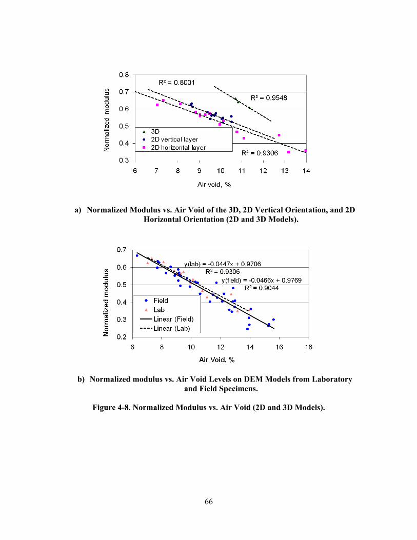
66
a) Normalized Modulus vs. Air Void of the 3D, 2D Vertical Orientation, and 2D Horizontal Orientation (2D and 3D Models).
b) Normalized modulus vs. Air Void Levels on DEM Models from Laboratory
and Field Specimens.
Figure 4-8. Normalized Modulus vs. Air Void (2D and 3D Models).
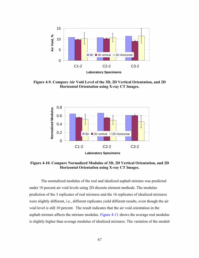
67
Figure 4-9. Compare Air Void Level of the 3D, 2D Vertical Orientation, and 2D
Horizontal Orientation using X-ray CT Images.
Figure 4-10. Compare Normalized Modulus of 3D, 2D Vertical Orientation, and 2D
Horizontal Orientation using X-ray CT Images.
The normalized modulus of the real and idealized asphalt mixture was predicted
under 10 percent air void levels using 2D discrete element methods. The modulus
prediction of the 3 replicates of real mixtures and the 16 replicates of idealized mixtures
were slightly different, i.e., different replicates yield different results, even though the air
void level is still 10 percent. The result indicates that the air void orientation in the
asphalt mixture affects the mixture modulus. Figure 4-11 shows the average real modulus
is slightly higher than average modulus of idealized mixtures. The variation of the moduli
0
5
10
15
C1-2 C2-2 C3-2
Laboratoy specimens
Air
Void
, %3D 2D vertical 2D Horizontal
0
0.2
0.4
0.6
0.8
C1-2 C2-2 C3-2
Laboratoy specimens
Nor
mal
ized
mod
ulus
3D 2D vertical 2D Horizontal
Laboratory Specimens
Laboratory Specimens
Nor
mal
ized
Mod
ulus
A
ir Vo
id, %

68
predicted from the 2D real models is lower than the 2D idealized model. Figure 4-11 also
shows that the 3D mixture model predicts a higher modulus than the 2D mixture model.
Table 4-3. Parameters of 2D and 3D Models.
Specimen Specimen size
(dimension)
Element
number
Air
void
2D models from the
idealized specimen
80 x 40 mm 800 10%
2D models “cut” from a
real specimen
150 x 150 mm 262,144 10%
3D model (revised from
images of lab specimen)
50 x 50 x 164 mm 410,000 10%
Figure 4-11. Comparing Normalized Modulus of the Idealized Images, Real Images, and 3D Images.
2D Id
ealiz
ed
2D R
eal
3D
0.0
0.2
0.4
0.6
0.8
Specimens
Nor
mal
ized
mod
ulus
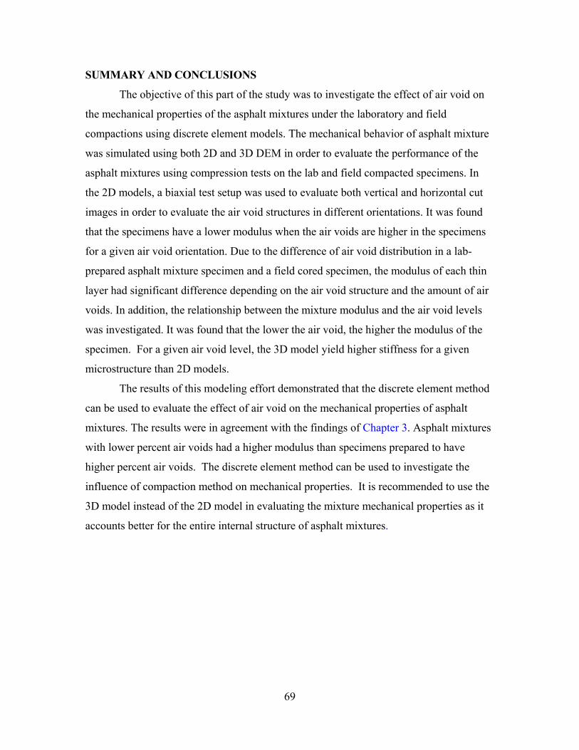
69
SUMMARY AND CONCLUSIONS
The objective of this part of the study was to investigate the effect of air void on
the mechanical properties of the asphalt mixtures under the laboratory and field
compactions using discrete element models. The mechanical behavior of asphalt mixture
was simulated using both 2D and 3D DEM in order to evaluate the performance of the
asphalt mixtures using compression tests on the lab and field compacted specimens. In
the 2D models, a biaxial test setup was used to evaluate both vertical and horizontal cut
images in order to evaluate the air void structures in different orientations. It was found
that the specimens have a lower modulus when the air voids are higher in the specimens
for a given air void orientation. Due to the difference of air void distribution in a lab-
prepared asphalt mixture specimen and a field cored specimen, the modulus of each thin
layer had significant difference depending on the air void structure and the amount of air
voids. In addition, the relationship between the mixture modulus and the air void levels
was investigated. It was found that the lower the air void, the higher the modulus of the
specimen. For a given air void level, the 3D model yield higher stiffness for a given
microstructure than 2D models.
The results of this modeling effort demonstrated that the discrete element method
can be used to evaluate the effect of air void on the mechanical properties of asphalt
mixtures. The results were in agreement with the findings of Chapter 3. Asphalt mixtures
with lower percent air voids had a higher modulus than specimens prepared to have
higher percent air voids. The discrete element method can be used to investigate the
influence of compaction method on mechanical properties. It is recommended to use the
3D model instead of the 2D model in evaluating the mixture mechanical properties as it
accounts better for the entire internal structure of asphalt mixtures.

70
71
CHAPTER 5
GUIDELINE FOR IMPROVING FIELD COMPACTION
INTRODUCTION
The findings from Report 0-5261-1 and this report showed that typically the air
void distribution is not uniform across the paving mat. The air void distribution correlated
very well with the compaction effort on the test section. The compaction effort was
presented by the number of roller passes and the location of each pass across the mat,
referred to as Compaction Index (CI). The efficiency of compaction at a given point is a
function of the location of this point with respect to the roller width. A point on the mat
closer to the center of the roller is subjected to more effective compaction than a point
closer to the edge of the roller. In addition, the air void distribution was found to be
influenced by the number of passes of the vibratory and static rollers compared to the
pneumatic one. The results also revealed a relationship between the compactability of
asphalt mixtures in the field and laboratory. For a given percent of air voids, the
compaction effort needed in the field correlated well with the slope of the laboratory
compaction curves. A higher compaction effort in the field was associated with a smaller
slope of the laboratory compaction curves. Based on these findings, the research team
submits some recommendations to improve the field compaction of asphalt mixtures. The
proposed recommendations can be applied during the mixture design and the construction
stages.
RECOMMENDATIONS DURING THE MIXTURE DESIGN STAGE
It is recommended to use the developed relationship between the slope of the
laboratory compaction curve and compaction index to decide on the field compactability
during the mixture design stage. This approach will ensure the mixtures can be
compacted in the field with required resistance to distresses that are associated with poor
compactability. The process of evaluating the compactability is illustrated in Figure 5-1,
and it is outlined in the following steps:

72
1) Compact the asphalt mixture using the Superpave gyratory compactor.
2) Plot the compaction curve (percent air voids versus number of gyrations) in a
semi log scale (Figure 5-1a).
3) Calculate the slope of the compaction curve between the initial compaction
point and the point at 8 percent air voids.
4) Use the relationship in Figure 5-1b to determine the CI.
5) Use Table 5-1 to determine the mixture compactability in the field.
6) If the mixture is in the difficult compactability region, the contractor can
choose to adjust the mixture design to improve the mixture compactability or
set up a compaction pattern and equipment in the field that can be used to
achieve the required compaction level (number of passes, sequence of
compaction, frequency, and amplitude of vibratory roller).
The research team is fully aware that the mixture compaction is influenced by the
type of equipment, the operations of the equipment, the mat temperature, and the air
temperature. The recommendations in Table 5-1 are based on the conditions used in the
field projects that were used in this study. However, our results show that the CI concept
applied reasonably well for all projects irrespective of the equipment used in these
projects. The recommendations in Table 5-1 should be used as initial guidelines as some
necessary adjustments can be made later as more field data about the influence of type of
equipment and the operational characteristics of the equipment on the results. It should be
noted that the required number of passes can be determined as the ratio of the compaction
index to the effectiveness factor at a point within the pavement mat.
We did not put recommendations on the field adjustments needed to achieve the
desired compaction level if the mixture falls under the “difficult compactability” level.
The contractor and highway agency personnel would be in a better position to make the
necessary plans and adjustments to achieve compactability given the prevailing site and
climatic conditions. However, the fact that a mixture belongs to the “difficult
compactability” should be treated as an indication that special efforts will be needed to
compact the mixture.
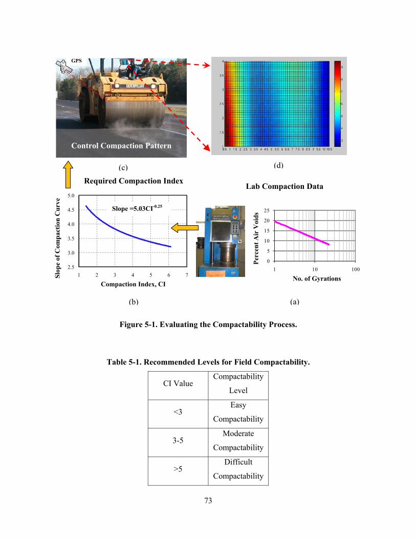
73
Figure 5-1. Evaluating the Compactability Process.
Table 5-1. Recommended Levels for Field Compactability.
CI Value Compactability
Level
<3 Easy
Compactability
3-5 Moderate
Compactability
>5 Difficult
Compactability
2.5
3.0
3.5
4.0
4.5
5.0
1 2 3 4 5 6 7Slop
e of
Com
pact
ion
Cur
ve
0
5
10
15
20
25
1 10 100
Compaction Index, CI
Control Compaction Pattern
No. of Gyrations
Perc
ent A
ir V
oids
GPS
Lab Compaction Data Required Compaction Index
(d)
(b) (a)
(c)
Slope =5.03CI-0.25

74
RECOMMENDATIONS DURING THE CONSTRUCTION STAGE
The findings showed that the efficiency of a steel wheel roller pass is not uniform
across its width. The efficiency in the middle 3 ft of a 7-ft wide roller has the full and
uniform effect. This efficiency decreases toward the edges of the roller. Uniform air void
distribution was found to be associated with a more uniform compaction index.
Researchers recommend the following steps during the construction stage:
1) Overhanging of the roller edge at a distance of about 1.5 ft to 2 ft from the
longitudinal joint. This way the longitudinal joint will experience the
maximum effectiveness of a given roller pass. Please note that, typically, the
edge of the mat or longitudinal joints is subjected to fewer roller passes.
Researchers found this overhanging of the roller at the joint can be done
without any problem for the restrained joints, but it might reduce the thickness
of the mat at the unrestrained or free joints. Consequently, it is recommended
to decrease the overhanging of the roller edge to about 1 ft at the unrestrained
joints or joints with very steep slope.
2) Overlapping between adjacent passes is recommended to be a minimum of
1.5 ft to 2 ft in order to achieve a uniform density across the width of the
roller. This overlapping of successive roller passes will ensure that every point
across the mat width experiences a minimum compaction index.
3) A compaction roller equipped with Geographic Information System (GIS) and
a simple software program can be used to guide the operator during the
construction to achieve the desired coverage. A system can be developed such
that the operator can see the real-time map of compaction index across the
width during compaction (Figure 5-1d). The operator can accordingly adjust
the successive pass and/or overlap to achieve uniform CI and uniform density
across the mat.
4) Use of the pneumatic tire compactor in the breakdown compaction would help
in achieving compaction in harsh mixtures that are difficult to compact.

75
CHAPTER 6
CONCLUSIONS AND RECOMMENDATIONS
CONCLUSIONS
A little effort was devoted in the past to study the factors that affect the
uniformity and level of compaction of asphalt pavements in the field. This study aimed at
providing such understanding in order to achieve more uniform asphalt pavements with
better performance. The effect of different levels of compaction on the mechanical
properties of asphalt pavements was also examined using a fracture mechanics approach
and Discrete Element Models. The fracture mechanics approach accounts for
fundamental material properties of asphalt mixtures, while the DEM models was used to
simulate the mechanical behavior of asphalt mixtures. The following points summarize
the main findings from this report.
Evaluation of Field Compaction
• The results of the three test sections evaluated in this part of the project agreed
with the findings from Report 0-5261-1.
• The air void distribution correlated well with the compaction effort across the
mat. The compaction effort was found to be a function of number of roller passes
and the location of each pass across the mat. Therefore, a new index referred as
the Compaction Index is proposed to quantify the compaction effort at any point
in the pavement. This index is the summation of the multiplication of each pass
with an effectiveness factor. The effectiveness factor at a point is a function of the
location of the point with respect to the roller width. A point on the mat closer to
the center of the roller is subjected to more effective compaction than a point
closer to the edge of the roller.
• The CI is used to study the compactability of asphalt mixtures in the field. The CI
correlated well with the slope of the laboratory compaction curves. Asphalt
mixtures with a higher slope in the laboratory needed less CI in the field to
achieve the same percent air void.
76
• It is demonstrated that the CI is useful to set up the compaction pattern in achieve
uniform percent air voids. A more uniform CI corresponds to more uniform air
voids across the mat.
• In most of the test sections, it was found that the middle part (across the depth) of
the mat is more compacted than the top and bottom parts.
Fracture Analysis of Moisture Damage
• The resistance of asphalt mixtures with different percent air voids to moisture
damage was evaluated by using a fracture mechanics approach in which a crack
growth index was used to quantify the damage of the test specimens.
• The analysis approach confirmed that the dry samples performed better than the
wet ones at each percent air voids.
• The test specimens with less percent air voids performed better than the ones with
higher percent air voids.
• The detrimental effect of moisture was the lowest at 7 percent air voids compared
with 4 and 10 percent air voids specimens.
Discrete Element Models of Mechanical Properties
• The effect of air void on the mechanical properties of asphalt mixtures was
investigated using discrete element models. The performance of asphalt mixtures
was simulated using both 2D and 3D DEM.
• For a given air void orientation, test specimens with less percent air voids have a
higher modulus compared to specimens at higher percent air voids.
• For a given air void level, the 3D model yield higher stiffness for a given
microstructure than 2D models.
RECOMMENDATIONS
The following are main recommendations based on the findings of this study:
1. Verify the relationship between laboratory compaction data and field
compaction by compacting more mixtures under different site and climatic

77
conditions. This additional effort will also validate the effectiveness
factors distribution and compaction index concept.
2. Develop a setup that can be used in the compaction equipment to monitor
and record the position of the roller with respect to the mat and the number
of passes across the different points in the mat. This data can be used to
plot the Compaction Index across the mat. The equipment operator can
then adjust the compaction pattern to achieve a uniform CI and
consequently a uniform distribution of air voids.
3. Evaluate the effect of different compaction rollers and operational
characteristics on the values of the compaction index, and make
adjustments to the recommendations in Table 5-1 to account for the type
of equipment is necessary. Our initial results suggest that the CI value is
not very sensitive to the type of equipment.

78
79
REFERENCES
Aboudi, J. (1991). “Mechanics of Composite Materials, a Unified Micromechanical
Approach,” Elsevier, 14-21.
Aboudi, J. (2004). “The generalized method of cells and high-fidelity generalized method
of cells micromechanical models – a review,” J. Mech. Adv. Mater. Struct, Vol. 11,
329-366.
American Association of State Highway and Transportation Officials (AASHTO).
(2002a). “Bulk Specific Gravity of Compacted Asphalt Mixtures Using Saturated
Surface-Dry Specimens.” T 166. Standard Specifications for Transportation
Materials and Methods Sampling and Testing, American Association of State
Highway and Transportation Officials, Washington, D.C.
American Association of State Highway and Transportation Officials (AASHTO).
(2002b). “Preparing and Determining the Density of Hot-Mix Asphalt (HMA)
Specimens by Means of the Superpave Gyratory Compactor.” T312. Standard
Specifications for Transportation Materials and Methods Sampling and Testing,
American Association of State Highway and Transportation Officials, Washington,
D.C.
American Association of State Highway and Transportation Officials (AASHTO).
(2007).“Standard Method of Test for Resistance of Compacted Asphalt Mixtures to
Moisture-Induced Damage.” T 283. Standard Specifications for Transportation
Materials and Methods Sampling and Testing, American Association of State
Highway and Transportation Officials, Washington, D.C.
Arambula, E. (2007). “Influence of Fundamental Material Properties and Air Void
Structure on Moisture Damage of Asphalt Mixes.” Ph.D. Dissertation, Texas A&M
University, College Station, Texas.

80
Buttlar W.G., and You, Z. (2001). “Discrete Element Modeling of Asphalt Concrete: A
Micro-Fabric Approach,” Journal of the Transportation Board, Washington, D.C.,
Vol. 1757.
Caro, S., Masad, E. Bahsin, A., and Little, D.N. (2007). “Moisture Susceptibility of
Asphalt Mixtures, Part 1: Mechanisms,” International Journal of Pavement
Engineering, submitted for publication.
Consuegra, A., Little, D.N., Quintus, H.V., and Burati, J. (1989). “Comparative
Evaluation of Laboratory Compaction Devices Based on Their Ability to Produce
Mixtures with Engineering Properties Similar to Those Produced in the Field,” In
Transportation Research Record 1228, TRB, National Research Council,
Washington, D.C., pp. 80-87.
Corps of Engineers (2000). “Hot-Mix Asphalt Paving Handbook 2000,” AC 150/5370-
14A, US Army Corps of Engineers, Washington, D.C.
Dai, Q., Sadd, M.H., and You, Z. (2006). “A Micromechanical Finite Element Model for
Viscoelastic Creep and Viscoelastic Damage Behavior of Asphalt Mixture,”
International Journal for Numerical and Analytical Methods in Geomechanics,
Vol. 30, 1135-1158.
Dai, Q., and You, Z. (2006). “Prediction of Creep Stiffness of Asphalt Mixture with
Micromechanical Finite Element and Discrete Element Models,” Journal of
Engineering Mechanics, ASCE, Vol. 133 (2), 163-173.
Flügge, W. (1975). “Viscoelasticity,” Berlin, Springer.
Harvey, J., and Monismith, C.L. (1993). “Effects of Laboratory Asphalt Concrete
Specimen Preparation Variables on Fatigue and Permanent Deformation Test
Results Using Strategic Highway Research Program A-003A Proposed Testing

81
Equipment,” In Transportation Research Record 1417, TRB, National Research
Council, Washington, D.C., pp. 38-57.
Howson, J., Masad, E., Bhasin, A., Branco, V., Arambula, E., Lytton, R., and Dallas, L.
(2007). “System for the Evaluation of Moisture Damage Using Fundamental
Material Properties.” Research Report FHWA/TX-07/0-4524-1, TTI, College
Station, Texas.
Image-Pro® Plus (1999). Media Cybernetics, L.P. Georgia, M.D. Version 4.1.
Itasca Consulting Group, PFC 2D Version 3.1. (2004a). Minneapolis, Minnesota.
Itasca Consulting Group, PFC 3D Version 3.1. (2004b). Minneapolis, Minnesota.
Li, G., Li, Y., Metcalf, J.B., and Pang S.S. (1999). “Elastic modulus prediction of asphalt
concrete,” Journal of Materials in Civil Engineering, Vol. 11(3), 236-241.
Lytton, R., Uzan, J., Fernando, E., Hiltmen, D., and Stoffels, S. (1993). “Development
and Validation of Perfomance Prediction Models and Specifications for Asphalt
Binder and Paving Mixtures,” SHRP A-357, Strategic Highway Research Program.
Washington, D.C.
Masad, E., Al-Omari, A., and Lytton, R. (2006a). “Simple Method for Predicting
Laboratory and Field Permeability of Hot Mix Asphalt,” In Transportation
Research Record 1970, TRB, National Research Council, Washington, D.C.,
pp. 55-63.
Masad, E., Zollinger, C., Bulut, R., Little, D., and Lytton, R. (2006b). “Characterization
of HMA Moisture Damage Using Surface Energy and Fracture Properties,”
Journal of the Association of Asphalt Paving Technologists, Vol. 75, pp. 713-748
82
Masad, E., Kassem, E., and Chowdhury, A. (2008). “Using Imaging Technology to
Improve the Laboratory and Field Compaction of Hot Mix Asphalt.” Technical
Report Number 0-5261-1, Texas Transportation Institute, Texas A&M University,
College Station, Texas.
Matlab Software (2004). The MathWorks Inc., Natick, Massachusetts, Version 7.
Nemat-Nasser, S., and Hori, M. (1999). “Micromechanics: Overall Properties of
Heterogeneous Materials,” 2nd ed. 1, North-Holland, Amsterdam.
Papagiannakis, A.T., Abbas, A., and Masad, E. (2002). “Micromechanical analysis of
viscoelastic properties of asphalt concretes,” Transportation Research Record,
Vol. 1789, pp: 113-120.
Peterson, B., Mahboub, K., Anderson, M., Masad, E., and Tashman, L. (2004).
“Comparing Superpave Gyratory Compactor Data to Field Cores,” Journal of
Materials in Civil Engineering, ASCE, Vol. 16(1), pp. 78-83.
Roberts F.L., Kandhal, P.S., Brown, E.R., Lee D., and Kennedy, T.W. (1996). “Hot Mix
Asphalt Materials, Mixture Design and Construction,” National Asphalt Pavement
Association, Research and Education Foundation, Lanham, Maryland.
Si, Z. (2001). “Characterization of Microdamage and Healing of Asphalt Concrete
Mixtures.” Ph.D. Dissertation, Texas A&M University, College Station, Texas.
Tashman, L., Masad, E., Peterson, B., and Saleh, H. (2001). “Internal Structure Analysis
of Asphalt Mixes to Improve the Simulation of Superpave Gyratory Compaction to
Field Conditions,” Journal of the Association of Asphalt Paving Technologists, Vol.
70, pp. 605-645.
83
Wolf, P., and Ghilani, C. (2002). Elementary Surveying: An Introduction to Geomatics,
10th Ed., Prentice Hall, Upper Saddle River, New Jersey.
You, Z., and Dai,Q. (2007). “Dynamic Complex Modulus Predictions of Hot-Mix
Asphalt Using a Micromechanical-Based Finite Element Model,” Canadian
Journal of Civil Engineering, Vol. 34(12), pp. 1519-1528.
You, Z., Adhikari, S., and Kutay, M.E. (2008). “Dynamic Modulus Simulation of the
Asphalt Concrete Using the X-ray Computed Tomography Images,” Materials and
Structures/Materiaux et Constructions, Vol. ISSN 1359-5997 (Print) 1871-6873
(Online), DOI 10.1617/s11527-007-9303-4.

84