Embed Size (px)
Citation preview

Atmos. Meas. Tech., 3, 209–232, 2010www.atmos-meas-tech.net/3/209/2010/© Author(s) 2010. This work is distributed underthe Creative Commons Attribution 3.0 License.
AtmosphericMeasurement
Techniques
A method for improved SCIAMACHY CO 2 retrieval in the presenceof optically thin clouds
M. Reuter, M. Buchwitz, O. Schneising, J. Heymann, H. Bovensmann, and J. P. Burrows
University of Bremen, Institute of Environmental Physics, P.O. Box 330440,28334 Bremen, Germany
Received: 28 August 2009 – Published in Atmos. Meas. Tech. Discuss.: 8 October 2009Revised: 15 January 2010 – Accepted: 9 February 2010 – Published: 12 February 2010
Abstract. An optimal estimation based retrieval scheme forsatellite based retrievals of XCO2 (the dry air column aver-aged mixing ratio of atmospheric CO2) is presented enablingaccurate retrievals also in the presence of thin clouds. Theproposed method is designed to analyze near-infrared nadirmeasurements of the SCIAMACHY instrument in the CO2absorption band at 1580 nm and in the O2-A absorption bandat around 760 nm. The algorithm accounts for scattering inan optically thin cirrus cloud layer and at aerosols of a defaultprofile. The scattering information is mainly obtained fromthe O2-A band and a merged fit windows approach enablesthe transfer of information between the O2-A and the CO2band. Via the optimal estimation technique, the algorithm isable to account for a priori information to further constrainthe inversion. Test scenarios of simulated SCIAMACHYsun-normalized radiance measurements are analyzed in orderto specify the quality of the proposed method. In contrast toexisting algorithms for SCIAMACHY retrievals, the system-atic errors due to cirrus clouds with optical thicknesses up to1.0 are reduced to values below 4 ppm for most of the ana-lyzed scenarios. This shows that the proposed method has thepotential to reduce uncertainties of SCIAMACHY retrievedXCO2 making this data product potentially useful for surfaceflux inverse modeling.
1 Introduction
CO2 is the dominant anthropogenic greenhouse gas but thereare still large uncertainties of its natural global sources andsinks (Stephens et al., 2007). Global measurements ofthe atmospheric CO2 concentration can be used as input
Correspondence to:M. Reuter([email protected])
for inverse models to reduce these uncertainties. In-situCO2 measurements of networks such as the NOAA (Na-tional Oceanic and Atmospheric Administration) carbon cy-cle greenhouse gas cooperative air sampling network (http://www.esrl.noaa.gov/gmd/ccgg/flask.html) are very accurate.However, the sparseness of the measurement sites and theirworld wide distribution with a majority over US and Euro-pean land surfaces and a minority on the Southern Hemi-sphere limit the current knowledge of CO2 surface fluxes.Theoretical studies have shown that satellite measurementsof CO2 have the potential to significantly reduce the surfaceflux uncertainties. This requires a precision of about 1% forregional averages and monthly means (Rayner and O’Brien,2001; Houweling et al., 2004). However, undetected biasesof a few tenths of a part per million on regional scales canalready hamper inverse surface flux modeling (Miller et al.,2007; Chevallier et al., 2007).
Currently, there are only a few satellite instruments in orbitwhich are able to measure atmospheric CO2. The High Res-olution Infrared Radiation Sounder (HIRS) (Chedin et al.,2002, 2003), the Atmospheric InfraRed Sounder (AIRS) (En-gelen et al., 2004; Engelen and McNally, 2005; Aumannet al., 2005; Strow et al., 2006; Maddy et al., 2008), andthe Infrared Atmospheric Sounding Interferometer (IASI)(Crevoisier et al., 2009) perform CO2 sensitive measure-ments in the thermal infrared (TIR) spectral region, i.e. theseinstruments do not detect reflected solar radiation but ther-mal radiation emitted from surface and atmosphere. Thisbrings the advantage that measurements are possible not onlyat day-time but also at night-time. However, the disadvantageof such measurements is their lack of sensitivity in the lowertroposphere where the strongest signals due to sources andsinks can be expected.
In contrast to this, the sensitivity of instruments measur-ing reflected solar radiation in the near-infrared (NIR)/short-wave infrared (SWIR) spectral region is much more constant
Published by Copernicus Publications on behalf of the European Geosciences Union.

210 M. Reuter et al.: A method for improved SCIAMACHY CO2 retrieval
(with height) and shows maximum values near the surface,typically. Note that in this paper NIR and SWIR are com-monly referred to as NIR. At present, SCIAMACHY aboardENVISAT launched in 2002 (Bovensmann et al., 1999) andTANSO (Thermal And Near infrared Sensor for carbonObservation) aboard GOSAT (Greenhouse gases ObservingSATellite) launched in 2009 (Yokota et al., 2004) are the onlyorbiting instruments measuring NIR radiation in appropriateabsorption bands at around 0.76, 1.6, and 2.0 µm with suf-ficient spectral resolution to retrieve XCO2. Another car-bon dioxide observing satellite was OCO (Orbiting CarbonObservatory) (Crisp et al., 2004). OCO was designed tomeasure within the same spectral region. Unfortunately, thesatellite was lost shortly after lift-off on 24 February 2009(Palmer and Rayner, 2009).
Contrary to TANSO, SCIAMACHY was not especiallydesigned for the retrieval of XCO2 with the precision and ac-curacy needed to enhance our knowledge about sources andsinks via inverse modeling. Due to SCIAMACHY’s lowerspatial and spectral resolution, the achievable accuracy andprecision is expected to be lower compared to a TANSO likeinstrument. Nevertheless, within the time period 2002–2009SCIAMACHY was the only instrument measuring XCO2from space with significant sensitivity also to the lower tro-posphere. Therefore, the development of algorithms derivingXCO2 from SCIAMACHY as accurate as possible with real-istic error estimates is crucial to start a consistent long-termtime series of XCO2 observations from space.
In the literature one can find several somewhat differ-ent XCO2 retrieval algorithms for SCIAMACHY data: TheWFM-DOAS algorithm (Weighting Function Modified Dif-ferential Optical Absorption Spectroscopy) was developed atthe University of Bremen for the retrieval of trace gases fromSCIAMACHY and has been described bySchneising et al.(2008), Buchwitz et al.(2005a,b, 2000b), andBuchwitz andBurrows(2004). This algorithm is based on a fast look-uptable (LUT) based forward model used to derive the num-ber of CO2 and O2 molecules in the atmospheric column inorder to derive XCO2. Other groups have developed some-what different approaches to retrieve XCO2 or CO2 columnsfrom SCIAMACHY. The computationally much more ex-pensive FSI/WFM-DOAS algorithm (Full Spectral InitiationWFM-DOAS) described by (Barkley et al., 2006a,c,b, 2007)derives XCO2 by retrieving the number of CO2 moleculesfrom SCIAMACHY but determining the air column frommeteorological analysis of the surface pressure. This ap-plies also to the algorithm discussed byHouweling et al.(2005). The retrieval algorithm designed for OCO followsthe strategy to determine XCO2 from column measurementsof CO2 and simultaneous measurements of the surface pres-sure derived from measurements in the O2-A band (Connoret al., 2008). Bosch et al.(2006) applied a modified ver-sion of this algorithm with a reduced number of state vec-tor elements to SCIAMACHY data in a surrounding of thePark Falls FTS-site. As SCIAMACHY’s channel 7 suffers
from a light-leak and ice on the detector, all these algorithmsderive the number of CO2 molecules from the weak CO2absorption band at around 1.6 µm and not from the muchstronger band at around 2.0 µm. Bosch et al.(2006) andSchneising et al.(2008) showed that XCO2 can be retrievedfrom SCIAMACHY with a single measurement precision of1–2% assuming clear sky conditions. Additionally,Schneis-ing et al. (2008) showed that a relative accuracy of about1–2% for monthly averages at a spatial resolution of about7◦
×7◦ can be achieved from SCIAMACHY measurementsunder clear sky conditions.
However, scattering at aerosol and/or cloud particles re-mains a major source of uncertainty for SCIAMACHYXCO2 retrievals which easily exceeds the precisions and ac-curacy estimated for clear sky conditions.Houweling et al.(2005) found that the XCO2 retrieval error may amount to10% in the presence of mineral dust aerosols.Schneisinget al.(2008) showed that a thin scattering layer with an opti-cal thickness of 0.03 in the upper troposphere can introduceXCO2 uncertainties of up to several percent. They deriveda XCO2 error of 8.80% resulting from a CO2 column errorof −0.89% and a O2 column error of−8.91% for a scenariowith an albedo of 0.1. Aben et al.(2007) found an underesti-mation of space-based measurements of the CO2 column of8% for a scenario with a cirrus cloud optical thickness (COT)of 0.05 and a surface albedo of 0.05. The underestimationamounted to 1% for an albedo of 0.5.
Unfortunately, thin clouds with optical thicknesses below0.1 cannot easily be detected within nadir measurements inthe visible and near infrared spectral region (e.g.Reuter et al.,2009; Rodriguez et al., 2007).
Satellite occultation measurements as well as lidar obser-vations show that sub visible cirrus clouds occur quite fre-quently with a maximum occurrence probability of about45% within the tropics, seasonally following the inter tropi-cal convergence zone (ITCZ) (Wang et al., 1996; Winker andTrepte, 1998; Nazaryan et al., 2008). The WFM-DOAS 1.0XCO2 retrieval for SCIAMACHY has a low quality overdark ocean surfaces and is therefore applied to land surfacesonly. The global distribution of the continents shows thatthe land masses of the Southern Hemisphere are closer tothe equator. For this reason, southern hemispheric SCIA-MACHY XCO2 retrievals are statistically much more af-fected by undetected sub visible cirrus clouds compared tonorthern hemispheric retrievals. Analyzing data of the li-dar instrument CALIOP (Cloud-Aerosol LIdar with Orthog-onal Polarization) aboard the CALIPSO satellite (Cloud-Aerosol Lidar and Infrared Pathfinder Satellite Observa-tions), Schneising et al.(2008) found that discrepancies ofthe southern hemispheric annual cycle of SCIAMACHY re-trieved XCO2 and corresponding values of NOAA’s CO2 as-similation system CarbonTracker (Peters et al., 2007) can bemost likely explained by sub visible cirrus clouds.
Atmos. Meas. Tech., 3, 209–232, 2010 www.atmos-meas-tech.net/3/209/2010/

M. Reuter et al.: A method for improved SCIAMACHY CO2 retrieval 211
Having in focus the spectrally high resolving satellite in-struments TANSO aboard GOSAT and OCO, algorithmshave been developed to correct for scattering effects.Brilet al. (2007) developed a method which is based on appli-cation of the equivalence theorem and photon path-lengthstatistics with further parameterization of the photon path-length probability density function (PPDF) for a TANSO likeinstrument. They derive effective scattering parameters ofcirrus clouds and aerosols from the O2-A band and from sat-urated water vapor lines at around 2.0 µm. This informationis used to correct the CO2 retrieval in the 1.6 µm CO2 band.Kuang et al.(2002) proposed a method based on simultane-ously fitting cloud and aerosol parameters (and others) withinthe three spectral bands of OCO at around 0.76, 1.6, and2.0 µm. They estimated that a precision of 0.3 to 2.5 ppm isachievable for aerosol optical thicknesses (AOT) of up to 0.3.
In contrast to both methods, the XCO2 retrieval algorithmsfor SCIAMACHY mentioned above do not explicitly ac-count for scattering effects. They either do not account forscattering at all or in an indirect way as the WFM-DOAS al-gorithm does by assuming that photon path-length modifica-tions are identical at 0.76 and 1.6 µm. In this approximation,scattering errors of CO2 and O2 cancel out when calculatingXCO2.
Within the publication at hand, a new XCO2 retrieval algo-rithm optimized for SCIAMACHY nadir data is introducedexplicitly considering scattering in an (optically thin) icecloud layer and at aerosols of a default profile. The physicalbasis for simultaneously retrieving scattering related param-eters and XCO2 using a merged fit windows approach is de-scribed in Sect.2. The information about these scattering pa-rameters comes mainly from the measurements in the O2 fitwindow. The usability of SCIAMACHY or GOME measure-ments in this spectral region for the retrieval of cloud param-eters is already confirmed within several publications (e.g.Kokhanovsky et al., 2006; Wang et al., 2008; van Dieden-hoven et al., 2007). Section3 describes the inversion tech-nique based on optimal estimation. Within this section, de-tails of the forward operator, the state vector, and the usageof prior knowledge is discussed. An error analysis is givenin Sect.4. Here, the retrieval algorithm is applied to simu-lated SCIAMACHY data in order to specify the algorithm’ssensitivity to the state vector elements but also to parametersthat are not retrieved within the state vector. In this regard,special emphasis is put on cloud parameters which are notretrieved.
2 Physical basis
The WFM-DOAS algorithm (Schneising et al., 2008; Buch-witz et al., 2005a,b, 2000b; Buchwitz and Burrows, 2004) re-trieves several independent parameters from SCIAMACHYmeasurements in the spectral region dominated by CO2absorption from 1558 to 1594 nm (in the following referred
to as the “CO2 fit window”) and also from measurements inthe spectral region of the O2-A band from 755 to 775 nm (inthe following referred to as the “O2 fit window”). Within theCO2 fit window the number of CO2 molecules, the number ofH2O molecules, the atmospheric temperature, spectral shiftand squeeze, and a 2nd order polynomial are retrieved. Thenumber of CO2 molecules is retrieved by shifting a referenceprofile with constant mixing ratio. In the same manner, thenumber of H2O molecules as well as the atmospheric tem-perature is determined by shifting reference profiles. Sep-arately from this, the number of O2 molecules, the atmo-spheric temperature, spectral shift and squeeze, and a 2ndorder polynomial are retrieved in an analogous way from theO2 fit window. Beforehand, an albedo retrieval is performedin both fit windows using measurements in micro windows(nearly) without absorptions line features at the edge of bothfit windows.
Each of these parameters influences the spectrum of re-flected solar radiation measured at the satellite instrument.The partial derivatives of the measured radiation with respectto a parameter is called the weighting function (or Jacobian)of this parameter. Of course, it is only possible to retrievethose parameters having a unique weighting function, suffi-ciently different from all other weighting functions in termsof the instrument’s precision. Very similar weighting func-tions can result in ambiguities of the retrieved correspondingparameters.
Figure 1 shows for exemplary atmospheric conditionswith moderate aerosol load and one thin ice cloud layerthe weighting functions of three different scattering re-lated parameters under a typical observation geometry inSCIAMACHY’s spectral resolution. Additionally, the figureshows the XCO2 weighting function which gives the changeof radiation when columnar increasing the CO2 concentra-tion by 1 ppm. For this example, the magnitude of its spectralsignature is comparable to a change of the cloud top height(CTH) by 1 km, the cloud water/ice path (CWP) by 0.2 g/m2,or to a change of the aerosol load by 100%. It is immedi-ately noticeable that there are high correlations between thecurves. Especially between the aerosol profile scaling (APS)and the cloud water/ice path weighting function as well as be-tween the cloud top height and the XCO2 weighting function.
XCO2 changes of 1 ppm are approximately the detectionlimit due to SCIAMACHY’s signal to noise (SNR) charac-teristics. This means, with SCIAMACHY it is actually notpossible to discriminate XCO2 values of a few ppm fromchanges of the given scattering parameters. For example, de-creasing the cloud top height from 14 to 10 km spectrallychanges the radiation in (nearly) the same way as increas-ing XCO2 by 4 ppm does. Most likely, it is not possible toretrieve scattering parameters simultaneously with the num-ber of CO2 molecules, i.e. uncertainties of the scattering pa-rameters will always result in uncertainties of the retrievedCO2 molecules when solely analyzing measurements fromthe CO2 fit window.
www.atmos-meas-tech.net/3/209/2010/ Atmos. Meas. Tech., 3, 209–232, 2010

212 M. Reuter et al.: A method for improved SCIAMACHY CO2 retrieval
cloud top height
1560 1570 1580 1590−1•10−5
0
1•10−5
2•10−5
3•10−5
4•10−5
5•10−5
∂I /
∂CT
H [k
m−
1 ]
cloud water path
1560 1570 1580 1590−0.0018
−0.0017
−0.0016
−0.0015
−0.0014
−0.0013
−0.0012
∂I /
∂CW
P [(
g/m
2 )−1 ]
XCO2
1560 1570 1580 1590wavelength [nm]
−4•10−5
−3•10−5
−2•10−5
−1•10−5
0
∂I /
∂XC
O2
[ppm
−1 ]
aerosol profile scaling
1560 1570 1580 1590wavelength [nm]
−4.9•10−4
−4.8•10−4
−4.7•10−4
−4.6•10−4
−4.5•10−4
−4.4•10−4
−4.3•10−4
∂I /
∂AP
S [A
PS
−1 ]
US−standard, SZA:40°, VZA:10°, albedo:0.2CWP:10g/m2, CGT:0.5km, Reff:50μm, CP:ice(fractals)
CTH:10km CTH:12km CTH:14km
Fig. 1. Weighting functions in the CO2 fit window for three cloud scenarios based on a US-standard atmosphere including an optically thinice cloud with a cloud top height of 10 km (blue), 12 km (black), and 14 km (red): cloud water/ice path (top/left), cloud top height (top/right),scaling of the aerosol profile (bottom/left), and XCO2 (bottom/right). The weighting functions are calculated with the SCIATRAN 3.0radiative transfer code and are folded with SCIAMACHY’s slit function.
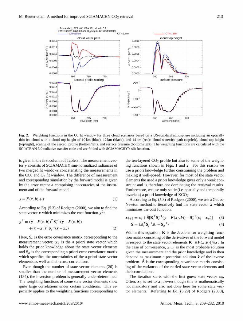
Analogous to Fig.1, Fig. 2 shows for identical atmo-spheric conditions the weighting functions of the same scat-tering parameters but for the O2 fit window. Additionally,it shows the weighting function in respect to surface pres-sureps which can be used to derive the total number of airmolecules within the atmospheric column by applying thehydrostatic assumption. The similarities between the weight-ing functions are less pronounced in this fit window. This ap-plies especially when comparing the surface pressure weight-ing function to the weighting functions of the given scatter-ing parameters. This originates by much stronger absorp-tion lines in this fit window. As width and depth of absorp-tion lines depend on the ambient pressure, saturation effectsdiffer much stronger with height within this spectral region.Additionally, SCIAMACHY’s resolution resolves the spec-tral structures of the gaseous absorption better within this fitwindow. Nevertheless, there are still similarities that are notnegligible e.g. between the cloud top height and aerosol pro-file scaling weighting function. Differences of 1 hPa are inthe order of the detection limit according to SCIAMACHY’sSNR characteristics. Therefore, it can be expected that inde-pendent information on the given scattering parameters canbe extracted from this fit window simultaneously with infor-mation about the surface pressure.
The large differences of the three illustrated cloud topheight weighting functions show that the radiative transfercan become non-linear in respect to this parameter. Addi-tionally, the spectral similarity of the CTH and the CWP
weighting function strongly depend on the scenario (largedifferences for the cloud at 12 km, minor differences for thecloud at 10 km). This means, depending on the individualscene, ambiguities may be more or less pronounced. In thiscontext, also the selected surface albedo has strong influence.
In the following section we will describe, how the infor-mation on scattering parameters, which can be derived fromthe O2 fit window, can be transported to the CO2 fit window.
3 Inversion via optimal estimation
We use an optimal estimation based inversion technique tofind the most probable atmospheric state given a SCIA-MACHY measurement and some prior knowledge. Nearlyall mathematical expressions given in this publication as wellas their derivation and notation can be found in the text bookof Rodgers(2000). A list of all used symbols is given byTable1.
The forward modelF is a vector function which calcu-lates for a given (atmospheric) state simulated measurementsi.e. simulated SCIAMACHY spectra. The input for the for-ward model are the state vectorx and the parameter vectorb.The state vector consists of all unknown variables that shallbe retrieved from the measurement (e.g. CO2). Parameterswhich are assumed to be exactly known but affecting the ra-diative transfer (e.g. viewing geometry) are the elements ofthe parameter vector. The entire list of state vector elements
Atmos. Meas. Tech., 3, 209–232, 2010 www.atmos-meas-tech.net/3/209/2010/
M. Reuter et al.: A method for improved SCIAMACHY CO2 retrieval 213
cloud top height
760 765 7700.0000
0.0002
0.0004
0.0006
0.0008
0.0010
∂I /
∂CT
H [k
m−
1 ]
cloud water path
760 765 7700.0007
0.0008
0.0009
0.0010
0.0011
0.0012
∂I /
∂CW
P [(
g/m
2 )−1 ]
surface pressure
760 765 770wavelength [nm]
−6•10−5
−4•10−5
−2•10−5
0
2•10−5
∂I /
∂SP
[hP
a−1 ]
aerosol profile scaling
760 765 770wavelength [nm]
0.0002
0.0004
0.0006
0.0008
0.0010
0.0012
0.0014
0.0016
∂I /
∂AP
S [A
PS
−1 ]
US−standard, SZA:40°, VZA:10°, albedo:0.2CWP:10g/m2, CGT:0.5km, Reff:50μm, CP:ice(fractals)
CTH:10km CTH:12km CTH:14km
Fig. 2. Weighting functions in the O2 fit window for three cloud scenarios based on a US-standard atmosphere including an opticallythin ice cloud with a cloud top height of 10 km (blue), 12 km (black), and 14 km (red): cloud water/ice path (top/left), cloud top height(top/right), scaling of the aerosol profile (bottom/left), and surface pressure (bottom/right). The weighting functions are calculated with theSCIATRAN 3.0 radiative transfer code and are folded with SCIAMACHY’s slit function.
is given in the first column of Table3. The measurement vec-tor y consists of SCIAMACHY sun-normalized radiances oftwo merged fit windows concatenating the measurements inthe CO2 and O2 fit window. The difference of measurementand corresponding simulation by the forward model is givenby the error vectorε comprising inaccuracies of the instru-ment and of the forward model:
y = F (x,b)+ε (1)
According to Eq. (5.3) ofRodgers(2000), we aim to find thestate vectorx which minimizes the cost functionχ2:
χ2= (y −F (x,b))T S−1
ε (y −F (x,b))
+(x −xa)T S−1
a (x −xa) (2)
Here,Sε is the error covariance matrix corresponding to themeasurement vector,xa is the a priori state vector whichholds the prior knowledge about the state vector elementsandSa is the corresponding a priori error covariance matrixwhich specifies the uncertainties of the a priori state vectorelements as well as their cross correlations.
Even though the number of state vector elements (26) issmaller than the number of measurement vector elements(134), the inversion problem is generally under-determined.The weighting functions of some state vector elements showquite large correlations under certain conditions. This es-pecially applies to the weighting functions corresponding to
the ten-layered CO2 profile but also to some of the weight-ing functions shown in Figs.1 and 2. For this reason weuse a priori knowledge further constraining the problem andmaking it well-posed. However, for most of the state vectorelements the used a priori knowledge gives only a weak con-straint and is therefore not dominating the retrieval results.Furthermore, we use only static (i.e. spatially and temporallyinvariant) a priori knowledge of XCO2.
According to Eq. (5.8) ofRodgers(2000), we use a Gauss-Newton method to iteratively find the state vectorx whichminimizes the cost function.
xi+1 = xi + S[KTi S−1
ε (y −F (xi,b))−S−1a (xi −xa)] (3)
S = (KTi S−1
ε K i +S−1a )−1 (4)
Within this equation,K is the Jacobian or weighting func-tion matrix consisting of the derivatives of the forward modelin respect to the state vector elementsK=∂F (x,b))/∂x. Inthe case of convergence,xi+1 is the most probable solutiongiven the measurement and the prior knowledge and is thendenoted as maximum a posteriori solutionx of the inverseproblem. S is the corresponding covariance matrix consist-ing of the variances of the retried state vector elements andtheir correlations.
The iteration starts with the first guess state vectorx0.Often, x0 is set toxa , even though this is mathematicallynot mandatory and also not done here for some state vec-tor elements. Referring to Eq. (5.29) ofRodgers(2000),
www.atmos-meas-tech.net/3/209/2010/ Atmos. Meas. Tech., 3, 209–232, 2010

214 M. Reuter et al.: A method for improved SCIAMACHY CO2 retrieval
Table 1. List of used symbols and corresponding dimensions andshort descriptions.
Symbol Dimension Description
αλ 1 Albedo (wavelength dependent)A n×n Averaging kernel matrixb nb×1 Parameter vectordl 1 Degree of non-linearityds 1 Degree of freedom for signalε m×1 Measurement and forward model errorF m×1 Forward modelG n×m Gain matrixK m×n Weighting function matrixH 1 Information content in bitsλ 1 Wavelengthλc 1 Center wavelength of a fit windowλmax 1 Maximum wavelength of a fit windowλmin 1 Minimum wavelength of a fit windowm 1 Size of measurement vector (=134)n 1 Size of state vector (=26)nb 1 Size of parameter vectornCO2 1 CO2 profile layers (=10)P 1 Polynomial coefficientps 1 Surface pressurerσ n×1 Uncertainty reductionS n×n Covariance matrix of retrieved stateSa n×n A priori covariance matrixSε m×m Measurement error covariance matrixw n×1 Layer weighting vectorx n×1 State vectorx0 n×1 First guess state vectorxa n×1 a priori state vectorxt n×1 True state vectorx n×1 Retrieved state vectorχ2 1 Cost function (Eq.2)y m×1 Measurement vector
we test for convergence by relating the changes of the statevector to the error covarianceS after each iteration. If thevalue of(xi−xi+1)
T S−1(xi−xi+1) falls below the numberof state vector elements (26), we assume that convergence isachieved and stop the iteration. As it is theoretically possiblethat convergence is never achieved, we stop the iteration afterten unsuccessful steps. However, typically, the convergencecriterion is fulfilled after two to four iterations.
Subsequently, we use some terms also given byRodgers(2000) to compute the gain matrixG (Eq. 2.45), the averag-ing kernel matrixA (Eq. 3.10), the degree of freedom for sig-nal ds (Eq. 2.80), and the information contentH (Eq. 2.80).The gain matrix corresponds to the sensitivity of the retrievalto the measurement and is given by:
G = (KT S−1ε K +S−1
a )KT S−1ε (5)
Having the gain matrix, we can compute the averaging kernelmatrix which is the sensitivity of the retrieval to the true state:
A = GK (6)
The degree of freedom for signal corresponds to the numberof independent quantities that can be derived from the mea-surement and is given by:
ds = tr(A) (7)
The information content gives the number of different atmo-spheric states that can be distinguished in bits:
H = −1
2ln(|I −A|) (8)
The degree of freedom as well as the information content canbe calculated for arbitrary sub sets of state vector elementsby taking only corresponding elements of the averaging ker-nel matrix into account. Comparing the variances of the re-trieved state vector elements with the corresponding a priorivariances, the uncertainty reductionrσ of thej th state vectorelement is defined by:
rσ j = 1−
√Sj,j/Saj,j (9)
Note: Using merged fit windows instead of performing aCO2 and a O2 retrieval independently within two separatefit windows has two main advantages when retrieving statevector elements which have sensitivities in both fit windows.1) These elements are better constrained because simultane-ous fitting implicitly utilizes the knowledge that the retrievedquantity (e.g. the atmospheric temperature) must be identi-cal in both fit windows. 2) If there are state vector elementswith strong ambiguities in one fit windows (e.g. surface pres-sure and scattering parameters in the CO2 fit window), theinformation come mainly from the fit window with less am-biguities. Merging the fit windows makes this informationavailable in both fit windows.
3.1 Forward model
All radiative transfer calculations utilized for our studies arecalculated with the SCIATRAN 3.0 radiative transfer code(Rozanov et al., 2005) in discrete ordinate mode. We use thecorrelated-k approach ofBuchwitz et al.(2000a) to increasethe computational efficiency. As final part of the forwardcalculation, the resulting spectra are folded with a SCIA-MACHY like Gaussian slit function and the dead/bad pixelmask also used for WFM-DOAS 1.0 is applied. Spectralline parameters are taken from the HITRAN 2008 (Rothmanet al., 2009) database.
The radiative transfer calculations are performed on 60model levels, even though our state vector includes onlya ten-layered CO2 mixing ratio profile. This profile is ex-panded to the model levels before each forward calculation.
Atmos. Meas. Tech., 3, 209–232, 2010 www.atmos-meas-tech.net/3/209/2010/

M. Reuter et al.: A method for improved SCIAMACHY CO2 retrieval 215
In the case of liquid water droplets, phase function, extinc-tion, and scattering coefficient of cloud particles are calcu-lated with Mie’s theory assuming gamma particle size distri-butions.
In the case of ice crystals, corresponding calculations areperformed with a Monte Carlo code, assuming an ensembleof randomly aligned fractal or hexagonal particles. The vol-ume scattering function is the product of phase function andscattering coefficient. Figure3 illustrates the volume scatter-ing functions of all cloud particles analyzed in Sect.4.
3.2 State vector
All retrieval results shown here are valid for a state vectorconsisting of 26 elements listed in the first column of Ta-ble 3. Corresponding weighting functions calculated for ex-emplary atmospheric conditions are illustrated in Fig.4. Thisfigure shows that not only the scattering parameter weightingfunctions may have cross correlations with other weightungfunctions. In this context, e.g. the albedo weighting functionsshow strong similarities to the scattering related weightingfunctions. For all state vector elements, we aim at obtainingrealistic a priori uncertainties which sufficiently constrain theinversion by defining a well-posed problem without dominat-ing the retrieval results.
3.2.1 Wavelength shift, slit function FWHM
The state vector accounts for fitting a wavelength shift andthe full width half maximum (FWHM) of a Gaussian shapedinstrument’s slit function separately in the O2 and CO2 fitwindow. This means, the corresponding weighting functionsare identical zero within the O2 or in the CO2 fit window,respectively.
3.2.2 Albedo
We assume a Lambertian surface with an albedoα withsmooth spectral progression which can be expressed by a 2ndorder polynomial separately within both fit windows.
αλ = P0+P1λ−λc
λmax−λmin+P2(
λ−λc
λmax−λmin)2 (10)
Here,P0, P1, andP2 are the polynomial coefficients,λ thewavelength,λc the center wavelength,λmin the minimum,andλmax the maximum wavelength within the fit window. Inorder to get good first guess and a priori estimates for the0th polynomial coefficients, we use the look-up table basedalbedo retrieval described bySchneising et al.(2008). Thisestimates the albedo within a micro window not influencedby gaseous absorption lines at one edge of each fit windowassuming a cloud free atmosphere with moderate aerosolload. We use an a priori uncertainty of 0.05 for the 0th poly-nomial coefficients. The first guess and the a priori valuesof the 1st and 2nd polynomial coefficients are zero. Their
0 45 90 135 180scattering angle [°]
0.0001
0.0010
0.0100
0.1000
1.0000
volu
me
scat
terin
g fu
nctio
n [s
r−1 m
−1 ]
water (λ=750nm)water (λ=1600nm)ice hex. (λ=750nm)ice hex.(λ=1600nm)ice frac. (λ=750nm)ice frac.(λ=1600nm)
6μm6μm12μm12μm50μm50μm
12μm12μm25μm25μm100μm100μm
18μm18μm50μm50μm300μm300μm
Fig. 3. Volume scattering functions of all cloud particles analyzedin Sect.4. The dominant forward peaks is cut in this clipping.
estimated a priori uncertainties are 0.01 and 0.001, respec-tively. The magnitude of these values is typical for 2nd orderpolynomial coefficients fitted to the natural surfaces albedosshown in Fig.5.
3.2.3 CO2 mixing ratio profile
The CO2 mixing ratio is fitted within 10 atmospheric layers,splitting the atmosphere in equally spaced pressure intervalsnormalized by the surface pressureps (0.0,0.1,0.2,...,1.0).
We analyzed CarbonTracker data over land surfaces of theyears 2003 to 2005 to determine a static a priori statistic forthe CO2 mixing ratio in corresponding pressure levels. Theresulting a priori state vector elements, their standard devi-ation and correlation matrix are shown in Fig.6. It is notsurprising that the largest variability is observed in the low-est 10% of the atmosphere. From the correlation matrix itis also visible that there are large cross correlations in theboundary layer, the free troposphere, and the stratosphere.
As the shape of the CO2 weighting functions in SCIA-MACHY resolution shows only minor changes with height,it cannot be expected that there is much information obtain-able about the CO2 profile shape from SCIAMACHY nadirmeasurements. Therefore, we use a relatively narrow con-straint for the profile shape but simultaneously a rather weakconstraint for XCO2. For this reason, we build the CO2 partof the a priori covariance matrix by using the correlation ma-trix as is but using a four times increased standard deviation.As a result, the a priori uncertainty of XCO2 increases from3.9 to 15.6 ppm. The average XCO2 of all analyzed Carbon-Tracker profiles amounts to 376.8 ppm.
www.atmos-meas-tech.net/3/209/2010/ Atmos. Meas. Tech., 3, 209–232, 2010

216 M. Reuter et al.: A method for improved SCIAMACHY CO2 retrieval
CO2 L0
CO2 L1
CO2 L2
CO2 L3
CO2 L4
CO2 L5
CO2 L6
CO2 L7
CO2 L8
CO2 L9
ps
CTH
CWP
APS
H2O
Δ T
FWHM (CO2)
FWHM (O2)
Δ λ (CO2)
Δ λ (O2)
Albedo P2 (CO2)
Albedo P1 (CO2)
Albedo P0 (CO2)
Albedo P2 (O2)
Albedo P1 (O2)
Albedo P0 (O2)
760 765 770 1560 1570 1580 1590
wavelength [nm]
Fig. 4. Weighting functions (scaled to the same amplitude) calculated with the SCIATRAN 3.0 radiative transfer code for the first guessstate vector of the “met. 1σ ” scenario at 40◦ solar zenith angle.
3.2.4 Atmospheric profiles
With regard to the application to real SCIAMACHY mea-surements, we plan to use atmospheric profiles of pressure,temperature, and humidity provided by ECMWF (EuropeanCenter for Medium-range Weather Forecasts) for the forwardmodel calculations as part of the parameter vector. Applyingthe hydrostatic assumption, the surface pressure determinesthe total number of air molecules within the atmospheric col-umn. Therefore, it is a critical parameter for the retrieval ofXCO2.
We compared a dataset of more than 8000 radiosonde mea-surements of the year 2004 within−70◦ E to 55◦ E longitudeand−35◦ N to 80◦ N latitude with corresponding ECMWFprofiles. The exact SCIAMACHY sub pixel composition ofsurface elevations is not perfectly known. For this reason,we used unmodified ECMWF profiles i.e. we performed nointerpolation of the surface height within the ECMWF pro-files. Therefore, the surface elevation within a radiosondeprofile may differ from the surface elevation within the pro-file of the corresponding ECMWF grid box. This means,our estimate combines two uncertainties: The ECMWF sur-face pressure uncertainty and the sub grid box surface pres-sure variability due to topography which is most times muchlarger. This is only a rough estimate that certainly drasticallyoverestimates the true ECMWF surface pressure precisionfor cases where an interpolation to the true topography within
the instrument’s field of view can be applied. However, thisoverestimation ensures that we do not over constrain the re-trieval in respect to surface pressure.
Resulting from these comparisons, we estimated that thesurface pressure is known with a standard deviation of 3.2%.The standard deviation of the temperature shift between mea-sured and modeled temperature profiles amounts to 1.1 K.The corresponding value for a scaling of the H2O profile is32%. The biases were much smaller than the standard devia-tions. Therefore, we apply no bias to the a priori knowledgeof surface pressure, temperature profile shift, and scaling ofthe humidity profile.
3.2.5 Scattering parameters
Scattering can cause very complex modifications of the satel-lite observed radiance spectra and there is nearly an infi-nite amount of micro and macro physical parameters that areneeded to comprehensively account for all scattering effectsin the forward model. However, as illustrated in Figs.1 and2it is unlikely possible to retrieve many of these parameterssimultaneously from SCIAMACHY measurements in the O2fit window. The same applies to the CO2 fit window whichcontains even less information about these parameters.
We concentrate on three macro physical scattering param-eters having a dominant influence on the measured spec-tra. Their weighting functions contain sufficiently unique
Atmos. Meas. Tech., 3, 209–232, 2010 www.atmos-meas-tech.net/3/209/2010/

M. Reuter et al.: A method for improved SCIAMACHY CO2 retrieval 217
700 900 1100 1300 1500 1700wavelength [nm]
0.0
0.2
0.4
0.6
0.8
1.0
albe
do
snowsandconifers
oceansoildeciduous rangeland
Fig. 5. Spectral albedos of different natural surface types. Repro-duced from the ASTER Spectral Library through the courtesy ofthe Jet Propulsion Laboratory, California Institute of Technology,Pasadena, California (©1999, California Institute of Technology)and the Digital Spectral Library 06 of the US Geological Survey.
spectral signatures which makes them distinguishable fromother weighting functions. These parameters are cloud topheight, cloud water/ice path whereas water/ice stands for iceand/or liquid water, and the aerosol scaling factor for a de-fault aerosol profile. All other scattering related parametersare not part of the state vector but only part of the parametervector and are set to constant values.
Within the parameter vector we define that scattering atparticles takes place in a plane parallel geometry at onecloud layer with a geometrical thickness of 0.5 km homo-geneously consisting of fractal ice crystals with 50 µm ef-fective radius. In addition, scattering happens at a stan-dard LOWTRAN summer aerosol profile with moderate ru-ral aerosol load and Henyey-Greenstein phase function and atotal aerosol optical thickness of about 0.136 at 750 nm and0.038 at 1550 nm. Both cloud parameters are aimed at opti-cally thin cirrus clouds because on the one hand it is not pos-sible to get enough information from below an optically thickcloud and on the other hand the foregoing cloud screening fil-ters already the optically thick clouds. Additionally,Schneis-ing et al.(2008) found that thin cirrus clouds are most likelythe reason for shortcoming of the WFM-DOAS 1.0 CO2 re-trieval on the Southern Hemisphere.
We set the a priori value of CTH to 10 km with a one sigmauncertainty of 5 km. Both values are only rough estimates fortypical thin cirrus clouds. Nevertheless, the size of the onesigma uncertainty seems to be large enough to avoid over-constraining the problem as it covers large parts of the uppertroposphere where these clouds occur.
All micro physical cloud and aerosol parameters are as-sumed to be constant and known. This assumption is obvi-ously not true. Scattering strongly depends on the size of thescattering particles e.g. scattering is more effective at clouds
280 330 380 430 480CO2 mixing ratio [ppm]
1.0
0.8
0.6
0.4
0.2
0.0
pres
sure
[ps]
xa 1σ 4σ
XCO2 [ppm]xa: 376.81σ: 3.894σ: 15.6
0.00
0.25
0.50
0.75
1.00
corr
elat
ion
1.0 0.8 0.6 0.4 0.2 0.0pressure [ps]
1.0
0.8
0.6
0.4
0.2
0.0
pres
sure
[ps]
Fig. 6. Static a priori knowledge of the ten-layered CO2 mixing ra-tio profile calculated from three years (2003–2005) CarbonTrackerdata over land surfaces. Top: A priori state vector values and their1σ and 4σ uncertainties. Bottom: Correlation matrix.
with smaller particles. For this reason, it is not possible toderive the correct cloud water/ice path without knowing thetrue phase function, scattering, and extinction coefficient ofthe scattering particles. Hence, the cloud water/ice path pa-rameter, which is part of our state vector, is rather an effectivecloud water/ice path corresponding to the particles defined inthe parameter vector. As an example, it can be expected thatthe retrieved CWP will be larger than the true CWP in caseswith true particles that are smaller than the assumed particles.Such effects must be considered when choosing the a pri-ori constraints of CWP. Additionally, the constraints must beweak enough to enable cloud free cases with CWP=0. Wehere use an a priori value for CWP of 5 g/m2 with an onesigma uncertainty of 10 g/m2. This corresponds to a cloudoptical thicknesses of the a priori cloud of 0.16. For theaerosol scaling factor we use an a priori value of 1.0 witha standard deviation of 1.0.
Obviously, three parameters are by far not sufficient to de-scribe all forms of scattering that can influence the SCIA-MACHY measurements. However, we are not aiming to re-trieve a very accurate and complete set of cloud or aerosolparameters. Therefore, we will address as major topic of
www.atmos-meas-tech.net/3/209/2010/ Atmos. Meas. Tech., 3, 209–232, 2010

218 M. Reuter et al.: A method for improved SCIAMACHY CO2 retrieval
Sect.4 the question how the lack of knowledge about sev-eral macro and micro physical cloud properties affects theXCO2 results.
3.3 XCO2
In this section we describe how XCO2 is calculated from theretrieved state vector elements and what implications this cal-culations have for the error propagation. As mentioned be-fore, the CO2 mixing ratio profile consists of ten layers withequally spaced pressure levels at(0.0,0.1,0.2,...,1.0)ps .Under the assumption of hydrostatic equilibrium, each layerconsists of the same number of air molecules. We define thelayer weighting vectorw as the fraction of air molecules ineach layer compared to the whole column. In our case itsvalue is always 0.1. For all elements that do not correspondto a CO2 mixing ratio profile element in the state vector, thelayer weighting vector is zero. XCO2 is than simply calcu-lated by:
XCO2=wT x (11)
Following the rules of error propagation, the variance of theretrieved XCO2 is given by:
σ 2XCO2
= wT Sw (12)
Note: the surface pressure weighting function is definedin that way, that a modification of the surface pressure in-fluences the number of molecules in the lowest layer only.This means, after an iteration that modifies the surface pres-sure, the surface layer will not have the same number of airmolecules anymore. The surface pressure weighting functionexpands or reduces the lowest layer assuming that this layerhas a CO2 mixing ratio given by the latter iteration or thefirst guess value. Therefore, the surface pressure weightingfunction influences the mixing ratio which is now a weightedaverage of the mixing ratio before and after iteration. For thisreason, at the end of each iteration, the new non-equidistantCO2 mixing ratio profile, which now starts at the updatedsurface pressure, is interpolated to ten equidistant pressurelevels whereas XCO2 is conserved.
4 Error analysis
Within the error analysis, the retrieval algorithm is appliedto SCIAMACHY measurements simulated with the forwardmodel described in Sect.3.1 using a modified US-standardatmosphere. The corresponding measurement error covari-ance matrices are assumed to be diagonal. They are cal-culated for an exposure time of 0.25 s using the instrumentsimulator that was also used for the calculations ofBuchwitzand Burrows(2004). However, it shall be noted that the cal-culated measurement errors are not utilized for adding noiseto the simulated spectra.
In the following, we analyze the retrieval’s capability toreproduce the state vector elements as well as the retrieval’s
sensitivity to cloud and aerosol related parameter vector ele-ments. Therefore, we define a set of 35 test scenarios. Someof them are only aiming at the retrieval’s capability to repro-duce changes of state vector elements.
However, radiative transfer through a scattering atmo-sphere can be very complex. Thinking about the almost in-finite number of possible ensembles of scattering particles,all with different phase functions, extinction, and absorptioncoefficients, a set of three scattering related state vector ele-ments is by far not enough to comprehensively describe allpossible scattering effects. For this reason, the remaining testscenarios are used to estimate the sensitivity to aerosol, cloudmicro and macro physical parameters which are not part ofthe state vector but of the parameter vector.
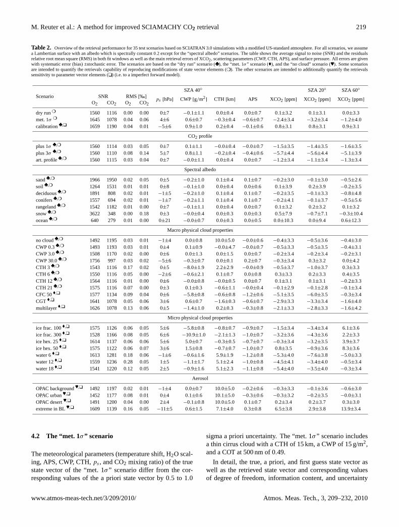
An overview of the results of all test scenarios is given inTable2 showing the systematic and stochastic XCO2 errorsof all scenarios for the solar zenith angles (SZA) 20◦, 40◦,and 60◦. Additionally, the systematic and stochastic errors ofthe scattering parameters and the surface pressure are givenfor 40◦ SZA. Except for the ”spectral albedo” scenarios, allcalculations are performed with an spectrally constant Lam-bertian albedo of 0.2. TableA1 and TableA2 include cor-responding results but for calculations with an albedo of 0.1and 0.3, respectively.
Note: The stochastic errors represent the a posteriori errorsbased on the assumed measurement noise and the assumed apriori error covariance matrix. According to Eq. (3.16) ofRodgers(2000), the systematic errors given in Table2 cor-respond to the smoothing error(A−I)(xt−xa) of the statevector elements. This applies to all scenarios in which onlystate vector elements but no parameter vector elements aremodified. In these cases, errors due to noise, unknown pa-rameter vector elements, and due to the forward model donot exist.
4.1 The “dry run” scenario
The true state vector of the “dry run” scenario is almost iden-tical to the first guess state vector which is again identical tothe a priori state vector in almost all elements. Only the con-stant part of the albedo polynomials of the first guess statevector differ slightly from the true state vector as it is esti-mated by the prior first guess albedo retrieval mentioned inSect.3.2.2. The “dry run” scenario includes a thin cirruscloud with a CTH of 10 km, a CWP of 10 g/m2, and a COTat 500 nm of 0.33.
Residuals with relative root mean square (RMS) values be-low 0.005‰ in the O2 and CO2 region as well as almost nosystematic errors prove that the algorithm is self-consistent(Table2).
The “dry run” scenario serves as basis for several otherscenarios which are mainly intended to quantify the retrievalscapability of reproducing modifications to a specific statevector element or to quantify the retrievals sensitivity to aspecific parameter vector element.
Atmos. Meas. Tech., 3, 209–232, 2010 www.atmos-meas-tech.net/3/209/2010/
M. Reuter et al.: A method for improved SCIAMACHY CO2 retrieval 219
Table 2. Overview of the retrieval performance for 35 test scenarios based on SCIATRAN 3.0 simulations with a modified US-standard atmosphere. For all scenarios, we assumea Lambertian surface with an albedo which is spectrally constant0.2 except for the “spectral albedo” scenarios. The table shows the average signal to noise (SNR) and the residualsrelative root mean square (RMS) in both fit windows as well as the main retrieval errors ofXCO2, scattering parameters (CWP, CTH, APS), and surface pressure. All errors are givenwith systematic error (bias) ±stochastic error. The scenarios are based on the “dry run” scenario (♣), the “met.1σ ” scenario (♦), and the “no cloud” scenario (♥). Some scenariosare intended to quantify the retrievals capability of reproducing modifications of state vector elements (❍). The other scenarios are intended to additionally quantify the retrievalssensitivity to parameter vector elements (❑) (i.e. to a imperfect forward model).
SZA 40◦ SZA 20◦ SZA 60◦
Scenario SNR RMS[‰]
O2 CO2 O2 CO2ps [hPa] CWP[g/m2
] CTH [km] APS XCO2 [ppm] XCO2 [ppm] XCO2 [ppm]
dry run❍ 1560 1116 0.00 0.00 0±7 −0.1±1.1 0.0±0.4 0.0±0.7 0.1±3.2 0.1±3.1 0.0±3.3met. 1σ ❍ 1645 1078 0.04 0.06 4±6 0.6±0.7 −0.3±0.4 −0.6±0.7 −2.4±3.4 −3.2±3.4 −1.2±4.0calibration♣,❑ 1659 1190 0.04 0.01 −5±6 0.9±1.0 0.2±0.4 −0.1±0.6 0.8±3.1 0.8±3.1 0.9±3.1
CO2 profile
plus 1σ ♣,❍ 1560 1114 0.03 0.05 0±7 0.1±1.1 −0.0±0.4 −0.0±0.7 −1.5±3.5 −1.4±3.5 −1.6±3.5plus 3σ ♣,❍ 1560 1110 0.08 0.14 5±7 0.8±1.1 −0.2±0.4 −0.4±0.6 −5.7±4.4 −5.6±4.4 −5.1±3.9art. profile♣,❍ 1560 1115 0.03 0.04 0±7 −0.0±1.1 0.0±0.4 0.0±0.7 −1.2±3.4 −1.1±3.4 −1.3±3.4
Spectral albedo
sand♣,❍ 1966 1950 0.02 0.05 0±5 −0.2±1.0 0.1±0.4 0.1±0.7 −0.2±3.0 −0.1±3.0 −0.5±2.6soil ♣,❍ 1264 1531 0.01 0.01 0±8 −0.1±1.0 0.0±0.4 0.0±0.6 0.1±3.9 0.2±3.9 −0.2±3.5deciduous♣,❍ 1891 808 0.02 0.01 −1±5 −0.2±1.0 0.1±0.4 0.1±0.7 −0.2±3.5 −0.1±3.3 −0.8±4.8conifers♣,❍ 1557 694 0.02 0.01 −1±7 −0.2±1.1 0.1±0.4 0.1±0.7 −0.2±4.1 −0.1±3.7 −0.5±5.6rangeland♣,❍ 1542 1182 0.01 0.00 0±7 −0.1±1.1 0.0±0.4 0.0±0.7 0.1±3.2 0.2±3.2 0.1±3.2snow♣,❍ 3622 348 0.00 0.18 0±3 −0.0±0.4 0.0±0.3 0.0±0.3 0.5±7.9 −0.7±7.1 −0.3±10.4ocean♣,❍ 640 279 0.01 0.00 0±21 −0.0±0.7 0.0±0.3 0.0±0.5 0.0±10.3 0.0±9.4 0.6±12.3
Macro physical cloud properties
no cloud♣,❍ 1492 1195 0.03 0.01 −1±4 0.0±0.8 10.0±5.0 −0.0±0.6 −0.4±3.3 −0.5±3.6 −0.4±3.0CWP 0.3♣,❍ 1493 1193 0.03 0.01 0±4 0.1±0.9 −0.0±4.7 −0.0±0.7 −0.5±3.3 −0.5±3.5 −0.4±3.1CWP 3.0♣,❍ 1508 1170 0.02 0.00 0±6 0.0±1.3 0.0±1.5 0.0±0.7 −0.2±3.4 −0.2±3.4 −0.2±3.1CWP 30.0♣,❍ 1756 997 0.03 0.02 −5±6 −0.3±0.7 0.0±0.1 0.2±0.7 −0.3±3.4 0.3±3.2 0.0±4.2CTH 3♣,❍ 1543 1116 0.17 0.02 0±5 −8.0±1.9 2.2±2.9 −0.0±0.9 −0.5±3.7 −1.0±3.7 0.3±3.3CTH 6♣,❍ 1550 1116 0.05 0.00 −2±6 −0.6±2.1 0.1±0.7 0.0±0.8 0.3±3.3 0.2±3.3 0.4±3.5CTH 12♣,❍ 1564 1116 0.01 0.00 0±6 −0.0±0.8 −0.0±0.5 0.0±0.7 0.1±3.1 0.1±3.1 −0.2±3.3CTH 21♣,❍ 1575 1116 0.07 0.00 0±3 0.1±0.3 −0.6±1.1 −0.0±0.4 −0.1±2.9 −0.1±2.8 −0.1±3.4CFC 50♦,❑ 1577 1134 0.09 0.04 0±6 −5.8±0.8 −0.6±0.8 −1.2±0.6 −5.1±3.5 −6.0±3.5 −0.3±3.4CGT♦,❑ 1641 1078 0.05 0.06 3±6 0.6±0.7 −1.6±0.3 −0.6±0.7 −2.9±3.3 −3.3±3.4 −1.6±4.0multilayer♦,❑ 1626 1078 0.13 0.06 0±5 −1.4±1.0 0.2±0.3 −0.3±0.8 −2.1±3.3 −2.8±3.3 −1.6±4.2
Micro physical cloud properties
ice frac. 100♦,❑ 1575 1126 0.06 0.05 5±6 −5.8±0.8 −0.8±0.7 −0.9±0.7 −1.5±3.4 −3.4±3.4 6.1±3.6ice frac. 300♦,❑ 1528 1166 0.08 0.05 6±6 −10.9±1.0 −2.1±1.3 −1.0±0.7 −3.2±3.6 −4.3±3.6 2.2±3.3ice hex. 25♦,❑ 1614 1137 0.06 0.06 5±6 5.0±0.7 −0.3±0.5 −0.7±0.7 −0.3±3.4 −3.2±3.5 3.9±3.7ice hex. 50♦,❑ 1575 1122 0.06 0.07 3±6 1.5±0.8 −0.7±0.7 −1.0±0.7 0.8±3.5 −0.9±3.6 8.3±3.6water 6♦,❑ 1613 1281 0.18 0.06 −1±6 −0.6±1.6 5.9±1.9 −1.2±0.8 −5.3±4.0 −7.6±3.8 −5.0±3.3water 12♦,❑ 1559 1236 0.28 0.05 1±5 −1.1±1.7 5.1±2.4 −1.0±0.8 −4.5±4.1 −3.4±4.0 −0.5±3.4water 18♦,❑ 1541 1220 0.12 0.05 2±5 −0.9±1.6 5.1±2.3 −1.1±0.8 −5.4±4.0 −3.5±4.0 −0.3±3.4
Aerosol
OPAC background♥,❑ 1492 1197 0.02 0.01 −1±4 0.0±0.7 10.0±5.0 −0.2±0.6 −0.3±3.3 −0.1±3.6 −0.6±3.0OPAC urban♥,❑ 1452 1177 0.08 0.01 0±4 0.1±0.6 10.1±5.0 −0.3±0.6 −0.3±3.2 −0.2±3.5 −0.0±3.1OPAC desert♥,❑ 1491 1200 0.04 0.00 2±4 −0.1±0.8 10.0±5.0 0.1±0.7 0.2±3.4 0.2±3.7 0.3±3.0extreme in BL♥,❑ 1609 1139 0.16 0.05 −11±5 0.6±1.5 7.1±4.0 0.3±0.8 6.5±3.8 2.9±3.8 13.9±3.4
4.2 The “met. 1σ ” scenario
The meteorological parameters (temperature shift, H2O scal-ing, APS, CWP, CTH,ps , and CO2 mixing ratio) of the truestate vector of the “met. 1σ ” scenario differ from the cor-responding values of the a priori state vector by 0.5 to 1.0
sigma a priori uncertainty. The “met. 1σ ” scenario includesa thin cirrus cloud with a CTH of 15 km, a CWP of 15 g/m2,and a COT at 500 nm of 0.49.
In detail, the true, a priori, and first guess state vector aswell as the retrieved state vector and corresponding valuesof degree of freedom, information content, and uncertainty
www.atmos-meas-tech.net/3/209/2010/ Atmos. Meas. Tech., 3, 209–232, 2010

220 M. Reuter et al.: A method for improved SCIAMACHY CO2 retrieval
0.00 0.05
0.10
0.15 0.20
760 765 770
−0.10
0.00
0.10
res[
%]
norm
.rad
.
SNR: 1645
RMS: 4.48e−03%
0.09
0.11
0.13
1560 1570 1580 1590wavelength [nm]
−0.20
0.00
0.20
res[
%]
norm
.rad
.
SNR: 1078
RMS: 5.86e−03%
meas.fit, residual
meas. err.first guess
Fig. 7. O2 and CO2 fit windows with simulated measurements,first guess, fitted sun-normalized radiation, residual and simulatedmeasurement uncertainty for the “met. 1σ ” scenario at 40◦ solarzenith angle.
reduction are given for this scenario in Table3. The cor-responding spectral fits in both fit windows as well as theirresiduals are plotted in Fig.7.
We find large uncertainty reductions greater than 0.88 forthe albedo parameters, wavelength shift, and FWHM withinthe O2 spectral region. The corresponding values of theCO2 spectral region are somewhat smaller but always greaterequal 0.69. Temperature shift and H2O scaling are retrievedwith low systematic biases and error reductions of 0.67 and0.79 despite rather narrow a priori constraints.
In contrast to this, the APS retrieval, with an uncertaintyreduction of only 0.32, seems to be dominated by the a pri-ori even though the corresponding constraints are weak. Ac-cordingly, we find a large stochastic error of 0.7 and a largesystematic bias of−0.6 which brings the retrieval close tothe a priori value. This can be explained by the following:The aerosol profile has its maximum in the boundary layerand scattering and absorption features of aerosol vary onlyslowly in the relatively narrow fit windows. Therefore, it isnot surprising that the shape of the APS weighting functionhas similarities to the surface pressure weighting function.Additionally, the sensitivity to APS is very low due to verylow absolute values of the APS weighting function. For bothpoints see Fig.2.
Compared to APS, the error reduction of CWP and CTHis much higher (>0.9). Referring to Fig.2, the shape of theCWP weighting function strongly depends on the specificscenario which can cause ambiguities, problems of finding
300 400 500 600CO2 mixing ratio [ppm]
1.0
0.8
0.6
0.4
0.2
0.0
pres
sure
[ps]
CO2 profile plus 1σCO2 profile plus 3σartificial CO2 profilea priori CO2 profile
truetruetruexa
retrievedretrievedretrieved1σ
Fig. 8. Retrieved and true CO2 mixing ratio profiles of the three“CO2 profile” scenarios.
suitable first guess values, and problems of the convergencebehavior. The retrieval’s sensitivity to CWP and CTH is de-scribed in more detail in Sect.4.6.
The surface pressure is retrieved with a bias of 4 hPa,a stochastic error of 6 hPa and an error reduction of 0.80.As the CO2 layered weighting functions look very similarand as the a priori knowledge shows strong inter-correlationbetween the layers, the retrieved profile has also stronglycorrelated layers. Additionally, the retrieval shows a verylow error reduction especially in the stratosphere resultingin a degree of freedom for signal of 1.07 for the whole pro-file. This means that only one independent information canbe retrieved about the profile. The shape of the profile re-mains strongly dominated by the a priori statistics. See alsoSects.4.4and4.9.
The “met. 1σ ” scenario serves as basis for several otherscenarios which are mainly intended to quantify the retrievalsperformance under more realistic conditions including alsounknown parameter vector elements, i.e. an imperfect for-ward model.
4.3 Calibration
The state vector of the WFM-DOAS algorithm includesa polynomial which accounts, among others, for spectrallysmooth variations of the surface albedo and for calibration er-rors causing a scaling of the sun-normalized radiance. Solelythe albedo retrieval of the WFM-DOAS algorithm relies onan absolute calibration. However, the WFM-DOAS albedoretrieval will produce unrealistic results in the presence ofclouds. For this reason, our method follows a slightly dif-ferent approach by fitting the albedo with a 2nd order poly-nomial. The “calibration” scenario estimates the influenceof calibration errors that cause an intensity scaling. For thispurpose, the simulated intensity of the “dry run” was scaled
Atmos. Meas. Tech., 3, 209–232, 2010 www.atmos-meas-tech.net/3/209/2010/

M. Reuter et al.: A method for improved SCIAMACHY CO2 retrieval 221
Table 3. Detailed retrieval results of the “met. 1σ ” scenario for each state vector element and for the resulting XCO2. The meaning ofthe columns from left to right is: 1) name of the state vector element, 2+3) weighting function with non-zero elements in the O2 and CO2fit window, respectively, 4) true statext , 5) first guess statex0, 6) a priori statexa ±uncertainty, 7) retrieved statex ±stochastic error, 8)information contentH , 9) degree of freedom for signalds , 10) uncertainty reductionrσ Note: xt , x0, xa , x, and the corresponding errorsare rounded to the same number of digits within each line.
Name O2 CO2 xt x0 xa x H [bit] ds rσ
AlbedoP0 • 0.200 0.224 0.224±0.050 0.202±0.002 4.65 1.00 0.96AlbedoP1 • 0.0000 0.0000 0.0000±0.0100 0.0000±0.0001 6.73 1.00 0.99AlbedoP2 • 0.0000 0.0000 0.0000±0.0010 0.0000±0.0001 3.09 0.99 0.88AlbedoP0 • 0.200 0.168 0.168±0.050 0.201±0.001 5.62 1.00 0.98AlbedoP1 • 0.0000 0.0000 0.0000±0.0100 0.0000±0.0002 5.63 1.00 0.98AlbedoP2 • 0.0000 0.0000 0.0000±0.0010 0.0001±0.0003 1.92 0.93 0.741λ [nm] • 0.000 0.000 0.000±0.100 0.000±0.000 9.14 1.00 1.001λ [nm] • 0.000 0.000 0.000±0.100 0.001±0.007 3.77 0.99 0.93FWHM [nm] • 0.450 0.450 0.450±0.050 0.450±0.000 6.76 1.00 0.99FWHM [nm] • 1.400 1.400 1.400±0.100 1.397±0.031 1.68 0.90 0.691T [K] • • −0.6 0.0 0.0±1.1 −0.8±0.4 1.62 0.89 0.67H2O [‰] • • 2.70 2.22 2.22±0.86 2.65±0.18 2.26 0.96 0.79APS • • 2.0 1.0 1.0±1.0 1.4±0.7 0.56 0.54 0.32CWP [g/m2] • • 15.0 10.0 5.0±10.0 15.6±0.7 3.85 1.00 0.93CTH [km] • • 15.0 10.0 10.0±5.0 14.7±0.4 3.59 0.99 0.92ps [hPa] • • 981 1013 1013±30 985±6 2.33 0.96 0.80CO2 L9 [ppm] • 380.9 373.0 372.9±8.0 375.4±7.5 0.01 0.01 0.06CO2 L8 [ppm] • 384.5 375.6 375.7±9.0 378.3±8.5 0.02 0.02 0.06CO2 L7 [ppm] • 385.1 376.4 376.4±8.6 380.9±7.3 0.03 0.04 0.16CO2 L6 [ppm] • 386.6 376.8 376.8±10.0 383.0±7.9 0.03 0.04 0.21CO2 L5 [ppm] • 387.9 377.0 377.0±11.1 384.0±8.7 0.03 0.05 0.22CO2 L4 [ppm] • 388.9 377.0 377.0±12.0 384.7±9.4 0.04 0.05 0.22CO2 L3 [ppm] • 390.0 377.1 377.1±13.1 385.7±10.2 0.04 0.05 0.22CO2 L2 [ppm] • 394.7 377.3 377.3±18.8 394.7±9.8 0.08 0.10 0.48CO2 L1 [ppm] • 409.3 377.6 377.6±36.4 411.5±18.5 0.17 0.21 0.49CO2 L0 [ppm] • 448.0 380.2 380.2±81.8 453.6±42.0 0.50 0.50 0.49
XCO2 [ppm] 395.6 376.8 376.8±15.6 393.2±3.4 2.46 1.07 0.78
by a factor by 10%. This primarily affects the retrieved0th order albedo polynomials which are approximately 10%too large. The weighting function of the 0th order albedopolynomial shows similarities with other weighting functions(Fig.4) which affects the retrieval errors of other parameters.However, the systematic errors of XCO2 remain smaller than1 ppm.
4.4 CO2 profile
The detailed results of the “met. 1σ ” scenario, given in Ta-ble 3, already show that it is not possible to retrieve muchinformation about the profile shape. Figure8 shows theretrieved CO2 profiles of the “plus 1σ ”, “plus 3σ ”, and“art. profile” CO2 profile scenarios. The three scenarios dif-fer from the “dry run” scenario only by a modified (true) CO2profile.
The “plus 1σ ” scenario has a true CO2 profile which dif-fers from the a priori profile by an enhancement of 1σ a prioriuncertainty in each layer. We find a slight overestimation of
the CO2 mixing ratio in the boundary layer, an almost neu-tral behavior between 0.8ps and 0.3ps , and a slight underes-timation in the stratosphere. The resulting XCO2 has a biasof −1.5 ppm and a stochastic error of 3.5 ppm for 40◦ SZA(Table2).
In the case of the “plus 3σ ” scenario, the observed effectsbecome more pronounced. We find a week overestimation inthe boundary layer, a week underestimation between 0.8ps
and 0.3ps , and a clear underestimation in the stratosphere.The resulting XCO2 has a bias of−5.7 ppm and a stochas-tic error of 4.4 ppm (Table2). Even though this scenariois a clear outlier in terms of the a priori statistics, the al-gorithm is still able to retrieve XCO2 with a systematic ab-solute error of 1.5%. This means that the XCO2 retrievalis still dominated by the measurement but not by the a pri-ori constraint. However, low uncertainty reductions in thestratospheric layers as well as the fact that the retrieved mix-ing ratios are much closer to the a priori than to the true pro-file show that the stratospheric layers are dominated by thea priori information and not by the measurement.
www.atmos-meas-tech.net/3/209/2010/ Atmos. Meas. Tech., 3, 209–232, 2010
222 M. Reuter et al.: A method for improved SCIAMACHY CO2 retrieval
In order to illustrate that it is actually not possible to re-trieve the shape of the CO2 profile, we confront the retrievalwith an artificial profile with an almost constant mixing ratioof 380 ppm in all layers except the third layer having a mix-ing ratio of about 495 ppm. In this case, the retrieved CO2profile follows not the true profile. In fact, the retrieved pro-file still adopts the shape from the a priori information eventhough the direction of the profile modification is retrievedcorrectly. However, the a priori information of the CO2 pro-file, which we generate from CarbonTracker data, hint thatthe profile shape is already relatively well known before themeasurement (Fig.6). Therefore, it is most unlikely that sce-narios like the “art. profile” scenario occur in reality.
Note that the systematic errors shown in this subsectioncorrespond to the CO2 profile smoothing error.
4.5 Spectral albedo
Unfortunately, the spectral albedo cannot be assumed to beconstant within the O2 and CO2 fit window. In the worst case,the spectral shape of the albedo would be highly correlatedwith the surface pressure or CO2 weighting function. In thiscase, errors of the retrieved surface pressure or CO2 mixingratios would be unavoidable. However, this is most unlikelyin reality.
As illustrated in Fig.5, the albedo of typical surface typesis spectrally smooth and only slowly varying within the fitwindows. This applies especially to satellite pixels withlarge foot print size consisting of a mixture of surface types.Therefore, we assume that the albedo can be approximatedwithin each fit window with a 2nd order polynomial. In or-der to make a perfect retrieval with no remaining residualstheoretically possible, we fit a 2nd order polynomial in bothfit windows to the spectral albedos given in Fig.5. We usethese polynomials as true spectral albedo for the albedo sce-narios “sand”, “soil”, “deciduous”, “conifers”, “rangeland”,“snow”, and “ocean”. All other elements of the state vectorare identical to those of the “dry run” scenario.
Table 2 shows that the systematic XCO2 errors of thesescenarios are all between−0.8 and 0.6 ppm, most of themclose to zero. We observe almost no systematic errors for thesurface pressure. According to the large differences of thetested albedos, SNR values vary from 640 to 3622 in the O2fit window and from 279 to 1950 in the CO2 fit window.
We find the lowest stochastic XCO2 errors for the “sand”scenario. This scenario has a relatively high albedo of about0.3 in the O2 and 0.5 in the CO2 fit window. For this reasonthe corresponding SNR values are also relatively large whichis essential for low stochastic errors.
The largest SNR values are observed in the O2 fit win-dow for the “snow” scenario because of the high reflectivityof snow in this spectral region. Due to the higher spectralresolution, stronger absorption features, and most times bet-ter SNR values in the O2 fit window, the surface pressureretrieval is dominated by the O2 fit window. For this reason,
we observe a distinctively smaller stochastic surface pressureerror of 3 hPa for this scenario. Nevertheless, the stochasticXCO2 error of this scenario is quite large with about 8 ppm.This can be explained by a very low SNR value in the CO2fit window caused by a very low reflectivity of snow in thisspectral region.
The “ocean” scenario has the lowest albedo and there-fore the lowest SNR value in the O2 and CO2 fit window.Consequently, we here observe the largest stochastic errorsof 21 hPa for the surface pressure and of about 10 ppm forXCO2. Comparing these values with the uncertainty of theprior knowledge shows that only very little information aboutXCO2 can be obtained over snow covered or ocean surfaces.
4.6 Macro physical cloud parameter
Within the scenarios “no cloud”, “CWP 0.3” to “CWP 30.0”,we test the retrievals ability to retrieve CWP of an ice cloudof fractal particles with 50 µm effective radius (as defined inthe parameter vector). All other state vector elements are de-fined as in the “dry run” scenario. As implied by the nameof these scenarios, the ice content of the analyzed cloudsamounts to 0.0, 0.3, 3.0, and 30.0 g/m2. The correspond-ing cloud optical thicknesses of these scenarios are about0.00, 0.01, 0.10, and 1.00. Note, in this context, specify-ing only the optical thickness is not appropriate to describethe scattering behavior of a cloud. Knowledge about phasefunction, extinction, and absorption coefficients is requiredin order to make the optical thickness a meaningful quantity.The SNR values of the “no cloud” and “CWP 0.3” scenar-ios is almost identical and there are only weak differencesto the “CWP 3.0” scenario. This indicates that the cloudsof these cases are extremely transparent and most likely notvisible for the human eye. In contrast to this, the SNR ofthe “CWP 30.0” scenario increases within the O2 fit window.Within the CO2 fit window, the effect of enhanced backscat-tered radiation is balanced by the strong absorption of ice inthis spectral region. We observe nearly no systematic errorsof the retrieved surface pressure except for the “CWP 30.0”scenario which results in a bias of−5 hPa. The CWP re-trieval is almost bias free compared to its stochastic error forall analyzed solar zenith angles. The same applies to the re-trieved CTH of the “CWP” scenarios. For the “no cloud”scenario, the unmodified a priori value is retrieved withoutany error reduction which is reasonable. The stochastic CTHerror reduces for CWP values greater than 3.0 g/m2. Thesystematic absolute XCO2 error of these scenarios is less orequal 0.5 ppm whereas the stochastic error is in the rangeof 3.0 and 4.2 ppm. In contrast to this, a WFM-DOAS likeretrieval systematically overestimates XCO2 by 3, 33, andmore than 400 ppm for the “CWP 0.3”, “CWP 3.0”, and“CWP 30.0” scenario, respectively. However, the WFM-DOAS 1.0 processing chain filters out cloud contaminatedscenarios like the latter. Note, the algorithm gets moreand more convergence problems for CWP values larger than
Atmos. Meas. Tech., 3, 209–232, 2010 www.atmos-meas-tech.net/3/209/2010/
M. Reuter et al.: A method for improved SCIAMACHY CO2 retrieval 223
30.0 g/m2 especially for large solar zenith angles. In suchcases, the algorithm is often not able to discriminate betweena thick cloud or an extremely low surface pressure.
Analogous to the “CWP” scenarios, the “CTH” scenariosare identical to the “dry run” scenario except for the cloudtop height which varies between 3, 6, 12, and 21 km. CWP,CTH, and APS are retrieved nearly bias free for the “CTH 6”,“CTH 12”, and “CTH 21” scenario. The systematic XCO2error of these scenarios is also comparatively low with valuesbetween−0.2 and 0.4 ppm. Only the “CTH 3” scenario pro-duces larger systematic errors of CWP and CTH. Addition-ally, the systematic XCO2 error of this scenario is slightlylarger with values up to−1.0 ppm. This behavior may be ex-plained by the fact that APS, and especially CTH and CWPweighing functions become more and more similar for lowclouds.
Up to this point, we only tested the retrieval’s ability toreproduce modifications to state vector elements. However,and as mentioned before, especially in respect to scattering,three state vector elements are by far not enough to entirelydefine the radiative transfer. For this reason, we analyze theretrieval’s sensitivity to different parameter vector elementswithin the following scenarios. At this, we put the emphasison properties of thin cirrus clouds. In the context of macrophysical cloud parameters we estimate the retrieval’s sensi-tivity to cloud fractional coverage of 50% (“CFC 50” sce-nario), cloud geometrical thickness (“CGT” scenario), andmultilayer clouds (“multilayer” scenario). These three sce-narios are based on the “met. 1σ ” scenario. They only differfrom their reference scenario by modified cloud properties.
The radiation of the “CFC 50” scenario is an average of theradiation of the “met. 1σ ” scenario with and without cloud.We observe a systematic CWP error being 6.4 g/m2 smallerthan the corresponding error of the “met. 1σ ” reference sce-nario. This can be explained with the total ice content ofthe “CFC 50” scenario which is 7.5 but not 15 g/m2. We re-trieve XCO2 values systematically differing in the range of−2.8 and 0.9 ppm from those of the reference scenario. Thisimplies that the errors induced by fractional cloud coveragemay also depend on CWP because the modeled cloud ap-pears thicker or thinner under different solar zenith angles.The total XCO2 errors are here in the range of−6.0 and−0.3 ppm.
The “CGT” scenario differs from the reference scenarioonly by the cloud geometrical thickness that is 2.5 km com-pared to 0.5 km for the reference scenario. The results ofthis scenario are very similar to the reference results. Solely,the retrieved CTH is systematically 1.3 km lower. Due to thelarger geometrical thickness and identical ice content at thesame time, the particle density is lower. For this reason, theeffective penetration depth in this cloud is larger which canexplain the differences of the retrieved CTH.
The “multilayer” scenario includes two clouds with iden-tical ice particles and identical geometrical thickness of0.5 km. The lower CTH is 8 km whereas the upper CTH is
12 km. The corresponding “true” value, which is the basisfor the calculation of the CTH bias in Table2, amounts to10 km. The results of this scenario are also comparable withthe results of the reference scenario. Systematic XCO2 dif-ferences compared to the reference scenario are in the rangeof −0.4 and 0.4 ppm. The retrieved CTH lies between thesimulated clouds and is 0.2 km larger than the average CTHof both cloud layers.
4.7 Micro physical cloud parameter
Within this section we estimate the retrieval’s sensitivity tocloud micro physical properties. This means, we confrontthe retrieval with clouds consisting of particles differing fromthose defined in the parameter vector.
The information about the three retrieved scattering pa-rameters CWP, CTH, and APS can nearly entirely be at-tributed to the O2 fit window. Scattering properties are de-fined within the state vector solely by these three parameters.The whole micro physical cloud and aerosol properties likephase function, extinction, and absorption coefficients areonly defined in the parameter vector. Unfortunately, thesemicro physical properties are not known and also not con-stant in reality and the values that we define in the parametervector are obviously only a rough estimate.
Let us first consider only the O2 fit window and assumethat extinction and absorption coefficients as well as phasefunction of the scattering particles are constant in this spec-tral region. Let us now assume two clouds having phasefunctions which differ only by a factor (or an offset withina logarithmic plot) outside the forward peak. In such case,the CWP retrieval would be ambiguous in respect to the mi-cro physical properties and consequently, correct CWP val-ues are only retrievable if the scattering particles are known.Referring to Fig.3, the volume scattering functions withinthe O2 fit window of e.g. fractal ice crystals of different sizeshow such similarities. This means that in the case of un-known particles, it is hardly possible to retrieve the true CWPfrom measurements in the O2 fit window only. The retrievedCWP is than rather an effective CWP under the assumptionof specific particles. Its value does not have to correspondto the true CWP. Note: The same applies to APS and also tosome extend to CTH. As long as the true geometrical thick-ness is known and defined in the parameter vector, the re-trieved CTH corresponds to the true CTH. Nevertheless, inreality the true cloud geometrical thickness is unknown andtherefore, only an effective CTH can be retrieved under theassumption of a cloud with 0.5 km geometrical thickness.This corresponds to the CTH results of the “CGT” scenarioin Table2.
www.atmos-meas-tech.net/3/209/2010/ Atmos. Meas. Tech., 3, 209–232, 2010

224 M. Reuter et al.: A method for improved SCIAMACHY CO2 retrieval
However, the effective scattering parameters are mainlyretrieved from the O2 fit window without knowledge of theactual micro physical properties. Therefore, the retrieved pa-rameters may not be appropriative for the usage in the CO2 fitwindow under some conditions. Particularly, this depends onthe relation of the absorption coefficients and volume scatter-ing functions within the O2 fit window compared to the CO2fit window. We can expect that the retrieved parameters areapplicable if this relation is similar for the true particles andthose particles that we assume within the parameter vector.
Assuming here a static relation is only a rough estimate,because methods like that ofNakajima and King(1990) arebased on the fact that liquid water droplets have a strongerabsorption at e.g. 1600 nm compared to e.g. 750 nm withnearly no absorption. This results in differences of the reflec-tion at clouds in both wavelengths which can be used to de-rive the cloud optical thickness and simultaneously the parti-cle’s effective radius. However, this method may fail for verythin clouds under conditions with unknown spectral albedo.Additionally, ice particles usually have non-spherical shapesinfluencing the corresponding phase functions. For these rea-sons, we did not consider to retrieve the cloud particle effec-tive radius simultaneously.
The clouds we use for the scenarios of this section, consistof fractal ice particles with 100 and 300 µm effective radius(“ice frac. 100” and “ice frac. 300” scenario), hexagonal iceparticles with 25 and 50 µm effective radius (“ice hex. 25”and “ice hex. 50” scenario), and water droplets with a gammaparticle size distribution and an effective radius of 6, 12, and18 µm, respectively (“water 6”, “water 12”, and “water 18”scenario). These scenarios are based on the “met. 1σ ” ref-erence scenario. The corresponding volume scattering func-tions are given in Fig.3.
For the most common shapes of cloud particles, a de-creasing particle size results in an increasing optical thick-ness and a decreasing forward peak of the phase function.For this reason we use different true CWP values for thesescenarios: 3 g/m2 for the “water” scenarios, 8 g/m2 for the“ice hex.” scenarios, and 15 g/m2 for the “ice frac.” sce-narios. Additionally we use different CTH values: 3 kmfor the “water” scenarios and 15 km, otherwise. The cor-responding cloud optical thicknesses (at 500 nm) are 0.25(“ice frac. 100”), 0.08 (“ice frac. 300”), 0.52 (“ice hex. 25”),0.29 (“ice hex. 50”), 0.80 (“water 6”), 0.39 (“water 12”), and0.26 (“water 18”).
The SNR values in the O2 fit window confirm, that moreradiation is scattered back from smaller particles. However,all values are in the rage of 1541 and 1614. Compared tothis, there is a relative large gap within the CO2 SNR valuesbetween the ice and water scenarios. This is caused by strongabsorption of ice in this spectral region which is often usedfor the retrieval of the cloud thermodynamic phase. This gap,however, indicates that statically defining all micro physicalcloud properties in the parameter vector must result in somemisinterpretations. In these cases, the enhanced or reduced
back scattered radiation is mainly misinterpreted as albedoeffect. Given a true albedo of 0.20 within both fit windows,the retrieved albedo varies between 0.20 and 0.22 within theO2 fit window and 0.20 and 0.23 within the CO2 fit window.For the retrieved surface pressure, we find systematic errorswhich are similar to the reference scenario.
The CWP behaves for ice particles as expected and showsnegative biases for particles larger than 50 µm and a posi-tive bias, otherwise. The results for water droplets are not soclear. Due to more pronounced differences in the shape ofthe volume scattering functions and absorption coefficients,we find for these scenarios increased RMS values of the re-sulting residuals. This especially applies to the O2 fit win-dow of the “water 12” scenario with a RMS value of 0.28‰.The corresponding expected RMS value due to SNR is about0.64‰.
For CTH, we find moderate negative biases for the an-alyzed ice particles which are comparable to the bias ofthe reference scenario. Only the “ice frac. 300” scenarioproduces a larger negative bias whereas the correspondingstochastic error hints at a lower sensitivity due to the reducedoptical thickness of this cloud. For the water cloud scenarios,we find large systematic biases of the CTH of up to 5.9 km.These may be explained by a rather low true CTH of 3 kmbeing far away from the a priori value of 10 km. Addition-ally, the profile of the aerosol extinction coefficient has itsmaximum values in the boundary layer so that misinterpreta-tions with APS may be possible here. Large systematic andstochastic errors are found for APS, showing that the APSretrieval is mainly driven by the a priori information but alsohinting that APS may easily be misinterpreted as CTH orCWP.
The systematic errors of the retrieved XCO2 are in therange of−7.6 and−0.9 ppm for 20◦ SZA,−5.4 and 0.8 ppmfor 40◦ SZA, and−5.0 and 8.3 ppm for 60◦ SZA. The cor-responding differences to the reference scenario are in therange of−4.4 and 2.3 ppm for 20◦ SZA, −3.0 and 3.2 ppmfor 40◦ SZA, and−3.8 and 9.5 ppm for 60◦ SZA. The in-creased errors at larger solar zenith angles can also be in-terpreted as errors due to enhanced cloud optical thickness.With increasing SZA, the light path through the cloud andtherefore also the apparent optical thickness of the cloudenhances. Vice versa, smaller systematic errors, which arecloser to those of the reference scenario, may be expectedfor lower CWP values.
4.8 Aerosols
Analogous to the cloud scenarios, we estimated the influ-ence of aerosol properties which are not part of the state vec-tor. For this purpose, we confront the algorithm with fouraerosol scenarios which are described in detail bySchneis-ing et al. (2008). Their profile, class of particles, andtheir phase function differ from the default aerosol scenario.The “OPAC background” scenario consists of continental
Atmos. Meas. Tech., 3, 209–232, 2010 www.atmos-meas-tech.net/3/209/2010/

M. Reuter et al.: A method for improved SCIAMACHY CO2 retrieval 225
relatively clean aerosol in the boundary layer and the freetroposphere. Its total aerosol optical thickness is 0.099 at750 nm and 0.026 at 1550 nm. The “OPAC urban” scenariohas continental polluted aerosol in the boundary layer andcontinental average aerosol in the free troposphere. Its to-tal aerosol optical thickness is 0.196 at 750 nm and 0.066at 1550 nm. The “OPAC desert” scenario consists of desertaerosol in the boundary layer and the continental cleanaerosol type in the free troposphere. Its total aerosol opticalthickness is 0.264 at 750 nm and 0.188 at 1550 nm. The “ex-treme in BL” scenario has strongly enhanced urban aerosol inthe boundary layer with a visibility of only 2 km and relativehumidity of 99%. Its total aerosol optical thickness is 2.528at 750 nm and 1.056 at 1550 nm. We used the “no cloud”scenario as basis for all aerosol scenarios. Except for theextreme scenario, all result are very similar to those of the“no cloud” reference scenario and the systematic absoluteXCO2 errors are below 0.6 ppm. In contrast to this, the ex-treme scenario produces much larger systematic errors whichare in the range of 2.9 ppm for 20◦ SZA and 13.9 ppm for 60◦
SZA.Schneising et al.(2008) performed a similar error esti-
mation but under slightly different conditions: They useda SZA of 50◦ and an albedo of 0.1 and found system-atic XCO2 errors of−3.8, −2.5, 1.3, and 21.7 ppm for the“OPAC background”, “OPAC urban”, “OPAC desert”, andthe “extreme in BL” scenario, respectively. Under theseconditions, we find systematic XCO2 errors of−0.6, −0.5,−0.6, and 10.6 ppm.
4.9 Column averaging kernel
The averaging kernel matrix gives the sensitivity of the re-trieval to the true state. Analogous to this, we define thecolumn averaging kernel vectoraCO2 as sensitivity of the re-trieved XCO2 to the true layered CO2 mixing ratios. In theideal case allnCO2 elements ofaCO2 would be equal 1. Thiswould mean that a XCO2 change introduced by a change oftheith layer is one-to-one reproduced by the retrieved XCO2.Considering only those state vector elementsi correspond-ing to the CO2 profile, the elements of the column averagingkernel vector can be calculated analogous toConnor et al.(2008) by:
(aCO2)i =∂XCO2
∂xi
1
wi
= (wT A)i1
wi
(13)
Figure9 shows the column averaging kernels of nine scenar-ios which differ by the solar zenith angles, albedo, and cloudwater/ice path. All nine scenarios are based on the “dry run”scenario. Except for the “alb. ocean” scenario, the retrievalshows a neutral sensitivity with averaging kernel values closeto unity within the lower troposphere i.e. within the lowestthree atmospheric layers. Within the upper atmosphere, theCO2 absorption lines become thinner and therefore deeperdue to the reduced ambient pressure so that saturation effects
0.2 0.4 0.6 0.8 1.0column averaging kernel
1.0
0.8
0.6
0.4
0.2
0.0
pres
sure
[ps]
SZACWPalbedo
20°0g/m2
sand
40°30g/m2
conifers
60°100g/m2
ocean
Fig. 9. Column averaging kernels of nine scenarios differing bythe solar zenith angles, albedo, and cloud water/ice path. All ninescenarios are based on the “dry run” scenario.
are more pronounced in the line centers. As a result theCO2 weighting functions show less sensitivity in the upperatmosphere. Additionally, the a priori constraints are muchtighter in this region. For these reasons, the averaging ker-nels of all analyzed cases reduce with height and minimumvalues between about 0.25 and 0.35 are found in the toplayer. This behavior is similar to that found byConnor et al.(2008). Only in the third atmospheric layer between 0.3ps
and 0.2ps , a considerable increase is observed for some sce-narios. Except for the CWP scenario with 0 g/m2, all illus-trated scenarios have an ice cloud in this layer. This increasesthe back scattered radiation and therefore also the sensitivityin the layers above the cloud. For bright surfaces, the rela-tive enhancement of radiation can be neglected. In contrast tothis, a major part of the detected radiation over dark surfacesis scattered at the cloud layer which increases the sensitivityabove the cloud. Accordingly, the effect is more pronouncedfor thicker clouds, higher solar zenith angles, and lower albe-dos. If the fraction of backscattered radiation at the cloudlayer is low enough, the effect is not observed at all.
4.10 Degree of non-linearity
If the forward model was perfectly linear in all state vector el-ements, the inversion would always converge within the firstiteration. However, in reality the forward model is more orless non-linear in respect to the state vector elements. The de-gree of non-linearitydl of a state vector elementi can be ex-pressed by evaluatingδy=F (x′
0,b)−F (x0,b)−K(x′
0−x0)
which is the difference ofF (x′
0,b) and the linear extrapo-lation of F (x0,b). Whereas,x′
0 differs fromx0 only in theith element. The difference is typically set to one standard
www.atmos-meas-tech.net/3/209/2010/ Atmos. Meas. Tech., 3, 209–232, 2010

226 M. Reuter et al.: A method for improved SCIAMACHY CO2 retrieval
Table 4. Degree of non-linearity of selected state vector elementscalculated for the “dry run” reference scenario. Given are the nameof the state vector element, the absolute deviation from the referencestate vector, the degree of non-linearity, and the absolute XCO2 er-ror when using a linear instead of the iterative retrieval.
Name |δxi | dl |δXCO2| [ppm]
AlbedoP0 (O2) 0.05 1.63 0.3AlbedoP0 (CO2) 0.05 0.37 0.21λ (O2) [nm] 0.10 11.70 13.31λ (CO2) [nm] 0.10 0.01 0.0FWHM (O2) [nm] 0.10 5.79 6.2FWHM (CO2) [nm] 0.10 0.02 0.01T [K] 1.1 0.97 0.0H2O [‰] 0.71 0.01 0.0APS 1.0 1.44 0.0CWP [g/m2] 10.0 16.20 0.0CTH [km] 5.0 5.17 2.1ps [hPa] 31 2.06 0.8XCO2 [ppm] 20.9 0.03 0.0
deviation.δy is than compared to the measurement error:
dl =
√δyT S−1
ε δy1
m(14)
This quantity is larger than unity if the spectral error dueto linearization exceeds the measurement error and smallerthan unity, otherwise. Nevertheless, large values ofdl doesnot necessarily have to result in large errors of the retrievedXCO2 because the spectral residual due to linearization doesnot have to correlate with any other weighting function. Onthe basis of Eq. (5.1) ofRodgers(2000), the error of the re-trieved state vector due to non-linearityδx when using a lin-ear retrieval instead of the iterative retrieval is about:
δx = G[F (x,b)−F (x0,b)−K(x −x0)] (15)
Analogous to Eq. (11) the corresponding XCO2 error is:
δXCO2=wT δx (16)
As an example, we calculateddl as well asδXCO2 for se-lected state vector elements for the “dry run” scenario ata SZA of 40◦. The results are given in Table4. Most ofthe analyzed state vector elements result in XCO2 errors lessthan 1 ppm which is much smaller than the stochastic errorof 3.2 ppm (Table2).
Several of the analyzed parameters have a degree of non-linearity greater than one but show only minor lineariza-tion errors for XCO2. This especially applies to CWP withdl=16.20 and|δXCO2|=0.0. The largest XCO2 linearizationerrors are observed for the non-atmospheric state vector el-ements of the O2 fit window: For the slit function’s FWHMand for the wavelength shift the XCO2 error amounts to 6.2and 13.3 ppm, respectively. However, the test interval of
0.1 nm is very large. For this reason, shift and squeeze of thewavelength axis is iteratively fitted in the WFM-DOAS 1.0retrieval, whereas linearity is assumed for all other fit param-eters. The largest XCO2 linearization errors of atmosphericparameters would occur when assuming linearity in respectto surface pressure (0.8 ppm), and CTH (2.1 ppm). This ac-cords with Fig.2 from which influences due to non-linearitiesof CTH were expected.
However, linearization errors in respect to CTH may be re-duced when fitting cloud top pressure instead of CTH. Thiscould reduce the number of needed iterations of an iterativeretrieval or reduce the errors of a non-iterative one-step re-trieval. In respect to the atmospheric gases H2O and CO2 theretrieval is very linear within the a priori uncertainty eventhough the retrieval uses the sun-normalized radiance but notits logarithm as input for the measurement vector. Note: Wehere analyze only one specific scenario and non-linearitiesmay be different under other conditions.
5 Conclusions
An optimal estimation based XCO2 retrieval scheme formeasurements in the O2-A band and in the weak CO2 ab-sorption band at 1580 nm has been presented. Its error char-acteristics have been analyzed for a SCIAMACHY like nadirlooking satellite instrument with moderate spectral resolu-tion. The proposed method is, however, not restricted toSCIAMACHY measurements and could be adapted to otherviewing geometries and spectral characteristics e.g. thoseof an upward looking ground-based NIR spectrometer. Weshowed that the retrieval of three scattering parameters fromtwo merged fit windows consisting of measurements in theO2 and CO2 band has the potential to drastically reduce sys-tematic XCO2 errors compared to a WFM-DOAS like re-trieval scheme which considers scattering only implicitly.The information about these parameters comes mainly fromthe O2 measurements and is made available in the CO2 bandby the merged fit windows approach. The retrieved scatteringparameters were: (effective) cloud water/ice path, (effective)cloud top height, and scaling factor for a default aerosol pro-file.
We found that only minor information is obtainable aboutthe scaling of the aerosol profile with error reductions ofabout 32%. However, in respect to a planned application toreal data, this state vector element enables us to use potentialprior knowledge about this parameter without disregardingthe available information.
Findings ofSchneising et al.(2008) hinted that sub visi-ble cirrus clouds are the major source of error of the WFM-DOAS 1.0 retrieval scheme. For this reason, we focused ouranalysis on optically thin ice clouds. The error reduction ofthe cloud parameters was much higher and amounted to over90% in most of the analyzed scenarios. We explained thiswith the fact that most of the analyzed clouds had a rather
Atmos. Meas. Tech., 3, 209–232, 2010 www.atmos-meas-tech.net/3/209/2010/

M. Reuter et al.: A method for improved SCIAMACHY CO2 retrieval 227
large cloud top height of 10 km or more which is typical forcirrus clouds. In this height, the spectral properties of oxy-gen can be distinguished from those near the surface withinthe simulated SCIAMACHY measurements.
The precision of the retrieved XCO2 was between 3 and4 ppm for most of the analyzed scenarios which is smallerbut similar to the 1–2% precision range experimentally deter-mined for the WFM-DOAS 1.0 retrieval scheme (Schneisinget al., 2008). Slightly lower values were observed for sce-narios with high albedo and therefore large signal to noisevalues. Much larger stochastic errors of up to 12.3 ppm wereobserved for low albedos of snow or open ocean.
The accuracy for scenes with optically thin cirrus cloudswas drastically enhanced compared to a WFM-DOAS likeretrieval. At solar zenith angles of 40◦, the presence of iceclouds with optical thicknesses in the range of 0.01 to 1.00contributed with less than 0.5 ppm to the systematic abso-lute XCO2 error if a perfect forward model is assumed. Thiscompares to systematic XCO2 errors of a WFM-DOAS likeretrieval scheme in the range of 3 ppm to more than 400 ppm.However, the WFM-DOAS 1.0 processing chain efficientlyfilters cloud contaminated scenes so that such large errors donot occur in the WFM-DOAS data product.
For scenarios with known parameter vector and withun-modified CO2 profile (“dry run”, “spectral albedo”,“no cloud”, “CWP”, and “CTH”), the systematic XCO2 er-rors were most times less than±0.5 ppm and always in therange of−1.0 and 0.6 ppm. XCO2 was systematically un-derestimated at scenarios with enhanced CO2 mixing ratioprofiles (e.g. “plus 1σ ”, “plus 3σ ”, and “art. profile”). Theunderestimation was interpreted as CO2 profile smoothingerror which results from lower sensitivities and lower a pri-ori uncertainties in respect to the CO2 mixing ratios in theupper atmosphere. The largest underestimation amounted to−5.7 ppm and occurred for the “plus 3σ ” scenario havinga considerably enhanced XCO2 of 439.4 ppm. This valuediffered from the a priori value by three times of the a prioriuncertainty which showed us that the XCO2 retrieval is dom-inated by the measurement but not by the a priori. Typicaluncertainty reductions of XCO2 were 78%.
Scattering in clouds was described by only two elementsof the state vector. For this reason, the retrieval’s sensitiv-ity to other scattering relevant (not retrieved) parameter vec-tor elements has been analyzed. These were micro physicalcloud properties like particle size, shape, and state of aggre-gation resulting in different phase functions, extinction, andabsorption coefficients. Due to more similar phase functions,the retrieval performed better and with smaller residuals forice clouds than for water clouds although lower CWP valueshave been used for the water clouds. The systematic XCO2errors of the “micro physical cloud properties” scenarios withice clouds were most times below±4 ppm. However, for wa-ter clouds and for some ice cloud scenarios with 60◦ solarzenith angle, larger systematic errors of up to 8.3 ppm wereobserved. In respect to (not retrieved) macro physical cloud
properties, we analyzed the retrieval’s sensitivity to multi-layer clouds, cloud geometrical thickness, and cloud frac-tional coverage. These properties contributed with−2.8 to0.9 ppm to the systematic XCO2 error. The largest effect wasobserved for the cloud fractional coverage.
Except for the “spectral albedo” scenarios, all scenarioswere calculated for a spectrally constant Lambertian albedoof 0.2. However, all calculations were repeated with analbedo of 0.1 and 0.3, respectively. As all scenarios had asemi transparent atmosphere, the albedo strongly influencedthe signal to noise ratios. As a result, the stochastic errorswere generally higher for an albedo of 0.1 and lower for analbedo of 0.3. Additionally, a dependency of the biases onthe surface albedo could be observed. The differences werelargest (up to 12 ppm) for the “micro physical cloud proper-ties” scenarios. Otherwise, only minor differences (for mostscenarios below 1 ppm) were observed. For the majority ofscenarios, the absolute values of the biases were reduced withincreasing albedo.
The column averaging kernels of the proposed method hadtheir maximum with values about 1.0 (except for one case) atthe surface layer. Higher in the atmosphere, a decreasing sen-sitivity was observed. Solely, above clouds that significantlycontribute to the total backscattered radiation, we observeda local maximum within the averaging kernels. Comparedto this, the averaging kernels of XCO2 retrieval schemes forTIR atmospheric sounders have their maximum in the higheratmosphere at around 210 hPa (Crevoisier et al., 2009). Theoptimal estimation technique could be utilized to use TIRbased CO2 retrievals as a prior knowledge which would fur-ther constrain the CO2 profile for pressure levels where NIRsensors have only a reduced sensitivity. This is affirmed byChristi and Stephens(2004) who found that TIR and NIRmeasurements complement one another in retrieving the CO2column.
The results presented here indicate that it is theoreticallypossible to retrieve XCO2 from SCIAMACHY nadir mea-surements with an accuracy and precision of about 1% inmany cases even in the presence of thin ice clouds. Thisrepresents an important step forward for the improvement ofXCO2 retrieval schemes for SCIAMACHY for the followingreasons: 1) Most cloud detection schemes are not able to de-tect sub visible cirrus clouds. 2) Rigorous masking of cloudswith optical thicknesses as small as 0.1 or lower would dras-tically reduce the amount of available data. 3) Large satellitepixels with sizes of 30 times 60 km have a high probabilityfor being cloud contaminated.
Using SCIATRAN as forward model makes the retrievalflexible but computational expensive. This hampers the ap-plication to large data amounts produced by SCIAMACHY.Therefore, investigations are ongoing to develop a lookup ta-ble approach based on pre calculated radiances which en-hances the computational efficiency at acceptable influenceson accuracy and precision.
www.atmos-meas-tech.net/3/209/2010/ Atmos. Meas. Tech., 3, 209–232, 2010
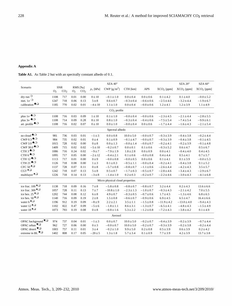
228 M. Reuter et al.: A method for improved SCIAMACHY CO2 retrieval
Appendix A
Table A1. As Table2 but with an spectrally constant albedo of 0.1.
SZA 40◦ SZA 20◦ SZA 60◦
Scenario SNR RMS[‰]
O2 CO2 O2 CO2ps [hPa] CWP[g/m2
] CTH [km] APS XCO2 [ppm] XCO2 [ppm] XCO2 [ppm]
dry run❍ 1108 717 0.01 0.00 0±10 −0.1±1.0 0.0±0.4 0.0±0.6 0.1±4.2 0.1±4.0 −0.0±5.2met. 1σ ❍ 1247 718 0.06 0.13 5±8 0.6±0.7 −0.3±0.4 −0.6±0.6 −2.5±4.6 −3.2±4.4 −1.9±6.7calibration♣,❑ 1185 770 0.02 0.01 −4±10 1.1±1.0 0.0±0.4 −0.0±0.6 1.2±4.1 1.2±3.9 1.1±4.9
CO2 profile
plus 1σ ♣,❍ 1108 716 0.03 0.09 1±10 0.1±1.0 −0.0±0.4 −0.0±0.6 −2.3±4.5 −2.1±4.4 −2.8±5.5plus 3σ ♣,❍ 1108 714 0.09 0.28 8±10 0.8±1.0 −0.3±0.4 −0.4±0.6 −7.5±5.4 −7.4±5.4 −9.9±6.1art. profile♣,❍ 1108 716 0.02 0.07 0±10 0.0±1.0 −0.0±0.4 0.0±0.6 −1.7±4.4 −1.6±4.3 −2.1±5.4
Spectral albedo
no cloud♣,❍ 981 736 0.03 0.01 −1±3 0.0±0.8 10.0±5.0 −0.0±0.7 −0.3±3.9 −0.4±3.8 −0.2±4.4CWP 0.3♣,❍ 984 735 0.02 0.01 0±4 0.1±0.9 −0.1±4.7 −0.0±0.7 −0.3±3.9 −0.4±3.8 −0.1±4.5CWP 3.0♣,❍ 1015 728 0.02 0.00 0±8 0.0±1.3 −0.0±1.4 −0.0±0.7 −0.2±4.1 −0.2±3.9 −0.1±4.8CWP 30.0♣,❍ 1409 715 0.02 0.02 −5±10 −0.2±0.7 0.0±0.1 0.1±0.6 −0.3±5.2 0.6±4.7 0.5±6.7CTH 3♣,❍ 1086 716 0.24 0.02 −9±7 −7.9±1.9 1.8±2.8 0.0±0.9 0.0±4.1 −0.4±4.0 0.4±4.5CTH 6♣,❍ 1095 717 0.05 0.00 −2±12 −0.4±2.1 0.1±0.6 −0.0±0.8 0.4±4.4 0.5±4.1 0.7±5.7CTH 12♣,❍ 1113 717 0.01 0.00 0±9 −0.0±0.8 −0.0±0.5 0.0±0.6 0.1±4.1 0.1±3.9 −0.0±5.3CTH 21♣,❍ 1126 718 0.08 0.00 1±3 0.1±0.3 −0.5±1.1 −0.0±0.4 −0.2±4.1 −0.4±3.8 0.1±5.2CFC 50♦,❑ 1137 728 0.07 0.11 0±8 −5.7±0.8 −0.8±0.7 −1.1±0.6 −2.6±4.4 −4.2±4.3 3.5±5.7CGT♦,❑ 1242 718 0.07 0.13 5±8 0.5±0.7 −1.7±0.3 −0.5±0.7 −2.8±4.6 −3.4±4.3 −2.9±6.7multilayer♦,❑ 1226 718 0.14 0.13 −3±8 −1.4±1.0 0.2±0.3 −0.2±0.7 −2.2±4.6 −3.0±4.3 −4.1±6.8
Micro physical cloud properties
ice frac. 100♦,❑ 1138 718 0.09 0.16 7±8 −5.8±0.8 −0.8±0.7 −0.8±0.7 3.2±4.4 0.2±4.3 13.6±6.6ice frac. 300♦,❑ 1057 728 0.11 0.13 7±7 −10.8±1.0 −2.3±1.3 −1.0±0.7 −0.3±4.3 −2.1±4.2 7.0±5.5ice hex. 25♦,❑ 1202 744 0.08 0.12 6±8 4.9±0.7 −0.3±0.5 −0.7±0.6 1.7±4.5 −1.3±4.6 6.8±6.5ice hex. 50♦,❑ 1140 716 0.09 0.19 2±8 1.5±0.8 −0.6±0.7 −0.9±0.6 6.9±4.5 6.5±4.7 16.4±6.6water 6♦,❑ 1196 912 0.19 0.09 −8±9 2.2±2.1 3.5±1.1 −1.5±0.8 −11.9±4.2 −13.0±4.0 −9.4±4.3water 12♦,❑ 1102 822 0.47 0.09 −5±6 −1.8±1.1 8.6±3.1 −1.3±0.7 −6.5±4.1 −4.8±4.3 −1.5±4.9water 18♦,❑ 1073 793 0.19 0.08 0±8 −0.8±1.6 5.3±2.2 −1.2±0.8 −7.2±4.3 −3.8±4.2 0.1±4.9
Aerosol
OPAC background♥,❑ 974 737 0.04 0.01 −1±3 0.0±0.7 10.0±5.0 −0.2±0.7 −0.4±3.9 −0.2±3.9 −0.7±4.4OPAC urban♥,❑ 962 727 0.06 0.00 0±3 −0.0±0.7 10.0±5.0 −0.2±0.7 −0.3±3.9 −0.2±3.8 −0.2±4.4OPAC desert♥,❑ 1003 757 0.11 0.01 3±4 −0.2±1.0 9.9±5.0 0.2±0.8 0.5±3.9 0.6±3.9 0.2±4.2extreme in BL♥,❑ 1402 808 0.17 0.05 −20±5 1.3±1.8 5.7±3.4 0.1±0.9 7.7±3.9 4.2±3.9 13.7±3.8
Atmos. Meas. Tech., 3, 209–232, 2010 www.atmos-meas-tech.net/3/209/2010/
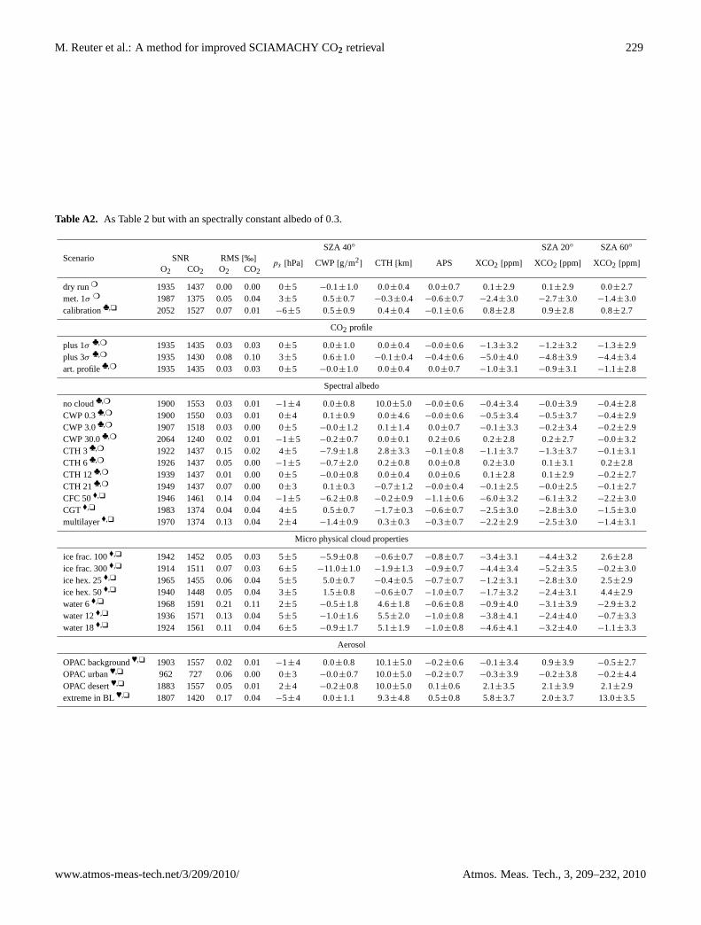
M. Reuter et al.: A method for improved SCIAMACHY CO2 retrieval 229
Table A2. As Table2 but with an spectrally constant albedo of 0.3.
SZA 40◦ SZA 20◦ SZA 60◦
Scenario SNR RMS[‰]
O2 CO2 O2 CO2ps [hPa] CWP[g/m2
] CTH [km] APS XCO2 [ppm] XCO2 [ppm] XCO2 [ppm]
dry run❍ 1935 1437 0.00 0.00 0±5 −0.1±1.0 0.0±0.4 0.0±0.7 0.1±2.9 0.1±2.9 0.0±2.7met. 1σ ❍ 1987 1375 0.05 0.04 3±5 0.5±0.7 −0.3±0.4 −0.6±0.7 −2.4±3.0 −2.7±3.0 −1.4±3.0calibration♣,❑ 2052 1527 0.07 0.01 −6±5 0.5±0.9 0.4±0.4 −0.1±0.6 0.8±2.8 0.9±2.8 0.8±2.7
CO2 profile
plus 1σ ♣,❍ 1935 1435 0.03 0.03 0±5 0.0±1.0 0.0±0.4 −0.0±0.6 −1.3±3.2 −1.2±3.2 −1.3±2.9plus 3σ ♣,❍ 1935 1430 0.08 0.10 3±5 0.6±1.0 −0.1±0.4 −0.4±0.6 −5.0±4.0 −4.8±3.9 −4.4±3.4art. profile♣,❍ 1935 1435 0.03 0.03 0±5 −0.0±1.0 0.0±0.4 0.0±0.7 −1.0±3.1 −0.9±3.1 −1.1±2.8
Spectral albedo
no cloud♣,❍ 1900 1553 0.03 0.01 −1±4 0.0±0.8 10.0±5.0 −0.0±0.6 −0.4±3.4 −0.0±3.9 −0.4±2.8CWP 0.3♣,❍ 1900 1550 0.03 0.01 0±4 0.1±0.9 0.0±4.6 −0.0±0.6 −0.5±3.4 −0.5±3.7 −0.4±2.9CWP 3.0♣,❍ 1907 1518 0.03 0.00 0±5 −0.0±1.2 0.1±1.4 0.0±0.7 −0.1±3.3 −0.2±3.4 −0.2±2.9CWP 30.0♣,❍ 2064 1240 0.02 0.01 −1±5 −0.2±0.7 0.0±0.1 0.2±0.6 0.2±2.8 0.2±2.7 −0.0±3.2CTH 3♣,❍ 1922 1437 0.15 0.02 4±5 −7.9±1.8 2.8±3.3 −0.1±0.8 −1.1±3.7 −1.3±3.7 −0.1±3.1CTH 6♣,❍ 1926 1437 0.05 0.00 −1±5 −0.7±2.0 0.2±0.8 0.0±0.8 0.2±3.0 0.1±3.1 0.2±2.8CTH 12♣,❍ 1939 1437 0.01 0.00 0±5 −0.0±0.8 0.0±0.4 0.0±0.6 0.1±2.8 0.1±2.9 −0.2±2.7CTH 21♣,❍ 1949 1437 0.07 0.00 0±3 0.1±0.3 −0.7±1.2 −0.0±0.4 −0.1±2.5 −0.0±2.5 −0.1±2.7CFC 50♦,❑ 1946 1461 0.14 0.04 −1±5 −6.2±0.8 −0.2±0.9 −1.1±0.6 −6.0±3.2 −6.1±3.2 −2.2±3.0CGT♦,❑ 1983 1374 0.04 0.04 4±5 0.5±0.7 −1.7±0.3 −0.6±0.7 −2.5±3.0 −2.8±3.0 −1.5±3.0multilayer♦,❑ 1970 1374 0.13 0.04 2±4 −1.4±0.9 0.3±0.3 −0.3±0.7 −2.2±2.9 −2.5±3.0 −1.4±3.1
Micro physical cloud properties
ice frac. 100♦,❑ 1942 1452 0.05 0.03 5±5 −5.9±0.8 −0.6±0.7 −0.8±0.7 −3.4±3.1 −4.4±3.2 2.6±2.8ice frac. 300♦,❑ 1914 1511 0.07 0.03 6±5 −11.0±1.0 −1.9±1.3 −0.9±0.7 −4.4±3.4 −5.2±3.5 −0.2±3.0ice hex. 25♦,❑ 1965 1455 0.06 0.04 5±5 5.0±0.7 −0.4±0.5 −0.7±0.7 −1.2±3.1 −2.8±3.0 2.5±2.9ice hex. 50♦,❑ 1940 1448 0.05 0.04 3±5 1.5±0.8 −0.6±0.7 −1.0±0.7 −1.7±3.2 −2.4±3.1 4.4±2.9water 6♦,❑ 1968 1591 0.21 0.11 2±5 −0.5±1.8 4.6±1.8 −0.6±0.8 −0.9±4.0 −3.1±3.9 −2.9±3.2water 12♦,❑ 1936 1571 0.13 0.04 5±5 −1.0±1.6 5.5±2.0 −1.0±0.8 −3.8±4.1 −2.4±4.0 −0.7±3.3water 18♦,❑ 1924 1561 0.11 0.04 6±5 −0.9±1.7 5.1±1.9 −1.0±0.8 −4.6±4.1 −3.2±4.0 −1.1±3.3
Aerosol
OPAC background♥,❑ 1903 1557 0.02 0.01 −1±4 0.0±0.8 10.1±5.0 −0.2±0.6 −0.1±3.4 0.9±3.9 −0.5±2.7OPAC urban♥,❑ 962 727 0.06 0.00 0±3 −0.0±0.7 10.0±5.0 −0.2±0.7 −0.3±3.9 −0.2±3.8 −0.2±4.4OPAC desert♥,❑ 1883 1557 0.05 0.01 2±4 −0.2±0.8 10.0±5.0 0.1±0.6 2.1±3.5 2.1±3.9 2.1±2.9extreme in BL♥,❑ 1807 1420 0.17 0.04 −5±4 0.0±1.1 9.3±4.8 0.5±0.8 5.8±3.7 2.0±3.7 13.0±3.5
www.atmos-meas-tech.net/3/209/2010/ Atmos. Meas. Tech., 3, 209–232, 2010
230 M. Reuter et al.: A method for improved SCIAMACHY CO2 retrieval
Acknowledgements.This study was funded by DLR-Bonn (grant50EE0507), ESA (ADVANSE project), the EU (FP7 MACC andCityZen), and the State and the University of Bremen, Germany.We thank NOAA for making available the CarbonTracker CO2fields and the radiosonde data. We thank ECMWF for providingthe meteorological data. We further thank our reviewers for theirhelpful and valuable comments to improve this work. Many thanksare given to S. Pfeifer and J. Reuter for proofreading the manuscript.
Edited by: G. Stiller
References
Aben, I., Hasekamp, O., and Hartmann, W.: Uncertainties in thespace-based measurements of CO2 columns due to scattering inthe Earth’s atmosphere, J. Quant. Spectrosc. Radiat. Transfer,104, 450–459, doi:10.1016/j.jqsrt.2006.09.013, 2007.
Aumann, H. H., Gregorich, D., and Gaiser, S.: AIRS hyper-spectral measurements for climate research: Carbon dioxideand nitrous oxide effects, Geophys. Res. Lett., 32, L05806,doi:10.1029/2004GL021784, 2005.
Barkley, M. P., Frieß, U., and Monks, P. S.: Measuring atmo-spheric CO2 from space using Full Spectral Initiation (FSI)WFM-DOAS, Atmos. Chem. Phys., 6, 3517–3534, 2006a,http://www.atmos-chem-phys.net/6/3517/2006/.
Barkley, M. P., Monks, P. S., and Engelen, R. J.: Comparison ofSCIAMACHY and AIRS CO2 measurements over North Amer-ica during the summer and autumn of 2003, Geophys. Res. Lett.,33, L20805, doi:10.1029/2006GL026807, 2006b.
Barkley, M. P., Monks, P. S., Frieß, U., Mittermeier, R. L., Fast,H., Korner, S., and Heimann, M.: Comparisons between SCIA-MACHY atmospheric CO2 retrieved using (FSI) WFM-DOAS toground based FTIR data and the TM3 chemistry transport model,Atmos. Chem. Phys., 6, 4483–4498, 2006c,http://www.atmos-chem-phys.net/6/4483/2006/.
Barkley, M. P., Monks, P. S., Hewitt, A. J., Machida, T., Desai, A.,Vinnichenko, N., Nakazawa, T., Yu Arshinov, M., Fedoseev, N.,and Watai, T.: Assessing the near surface sensitivity of SCIA-MACHY atmospheric CO2 retrieved using (FSI) WFM-DOAS,Atmos. Chem. Phys., 7, 3597–3619, 2007,http://www.atmos-chem-phys.net/7/3597/2007/.
Bosch, H., Toon, G. C., Sen, B., Washenfelder, R. A., Wennberg,P. O., Buchwitz, M., de Beek, R., Burrows, J. P., Crisp, D.,Christi, M., Connor, B. J., Natraj, V., and Yung, Y. L.: Space-based near-infrared CO2 measurements: Testing the OrbitingCarbon Observatory retrieval algorithm and validation conceptusing SCIAMACHY observations over Park Falls, Wisconsin,J. Geophys. Res., 111, D23302, doi:10.1029/2006JD007080,2006.
Bovensmann, H., Burrows, J. P., Buchwitz, M., Frerick, J., Noel, S.,Rozanov, V. V., Chance, K. V., and Goede, A.: SCIAMACHY –Mission Objectives and Measurement Modes, J. Atmos. Sci., 56,127–150, 1999.
Bril, A., Oshchepkov, S., Yokota, T., and Inoue, G.: Parameteri-zation of aerosol and cirrus cloud effects on reflected sunlightspectra measured from space: application of the equivalence the-orem, Appl. Opt., 46, 2460–2470, 2007.
Buchwitz, M. and Burrows, J. P.: Retrieval of CH4, CO, and CO2total column amounts from SCIAMACHY near-infrared nadirspectra: Retrieval algorithm and first results, in: Remote Sens-ing of Clouds and the Atmosphere VIII, edited by: Schafer, K.P., Comeron, A., Carleer, M. R., and Picard, R. H., Proceedingsof SPIE, 5235, 375–388, 2004.
Buchwitz, M., Rozanov, V. V., and Burrows, J. P.: A correlated-kdistribution scheme for overlapping gases suitable for retrievalof atmospheric constituents from moderate resolution radiancemeasurements in the visible/near-infrared spectral region, J. Geo-phys. Res., 105, 15247–15261, 2000a.
Buchwitz, M., Rozanov, V. V., and Burrows, J. P.: A near-infraredoptimized DOAS method for the fast global retrieval of atmo-spheric CH4, CO, CO2, H2O, and N2O total column amountsfrom SCIAMACHY Envisat-1 nadir radiances, J. Geophys. Res.,105, 15231–15245, 2000b.
Buchwitz, M., de Beek, R., Burrows, J. P., Bovensmann, H.,Warneke, T., Notholt, J., Meirink, J. F., Goede, A. P. H., Bergam-aschi, P., Korner, S., Heimann, M., and Schulz, A.: Atmosphericmethane and carbon dioxide from SCIAMACHY satellite data:initial comparison with chemistry and transport models, Atmos.Chem. Phys., 5, 941–962, 2005a,http://www.atmos-chem-phys.net/5/941/2005/.
Buchwitz, M., de Beek, R., Noel, S., Burrows, J. P., Bovensmann,H., Bremer, H., Bergamaschi, P., Korner, S., and Heimann,M.: Carbon monoxide, methane and carbon dioxide columns re-trieved from SCIAMACHY by WFM-DOAS: year 2003 initialdata set, Atmos. Chem. Phys., 5, 3313–3329, 2005b,http://www.atmos-chem-phys.net/5/3313/2005/.
Chedin, A., Hollingsworth, A., Scott, N. A., Serrar, S., Crevoisier,C., and Armante, R.: Annual and seasonal variations of at-mospheric CO2, N2O and CO concentrations retrieved fromNOAA/TOVS satellite observations, Geophys. Res. Lett., 29,1269, doi:10.1029/2001GL014082, 2002.
Chedin, A., Serrar, S., Scott, N. A., Crevoisier, C., and Armante, R.:First global measurement of midtropospheric CO2 from NOAApolar satellites: Tropical zone, J. Geophys. Res., 108, 4581,doi:10.1029/2003JD003439, 2003.
Chevallier, F., Breon, F.-M., and Rayner, P. J.: Contribu-tion of the Orbiting Carbon Observatory to the estimation ofCO2 sources and sinks: Theoretical study in a variationaldata assimilation framework, J. Geophys. Res., 112, D09307,doi:10.1029/2006JD007375, 2007.
Christi, M. J. and Stephens, G. L.: Retrieving profiles of at-mospheric CO2 in clear sky and in the presence of thincloud using spectroscopy from the near and thermal infrared:a preliminary case study, J. Geophys. Res., 109, D04316,doi:10.1029/2003JD004058, 2004.
Connor, B. J., Boesch, H., Toon, G., Sen, B., Miller, C., and Crisp,D.: Orbiting carbon observatory: Inverse method and prospec-tive error analysis, J. Geophys. Res.-Atmos., 113, D05305,doi:10.1029/2006JD008336, 2008.
Crevoisier, C., Chedin, A., Matsueda, H., Machida, T., Armante,R., and Scott, N. A.: First year of upper tropospheric integratedcontent of CO2 from IASI hyperspectral infrared observations,Atmos. Chem. Phys., 9, 4797–4810, 2009,http://www.atmos-chem-phys.net/9/4797/2009/.
Atmos. Meas. Tech., 3, 209–232, 2010 www.atmos-meas-tech.net/3/209/2010/

M. Reuter et al.: A method for improved SCIAMACHY CO2 retrieval 231
Crisp, D., Atlas, R. M., Breon, F.-M., Brown, L. R., Burrows, J. P.,Ciais, P., Connor, B. J., Doney, S. C., Fung, I. Y., Jacob, D. J.,Miller, C. E., O’Brien, D., Pawson, S., Randerson, J. T., Rayner,P., Salawitch, R. S., Sander, S. P., Sen, B., Stephens, G. L., Tans,P. P., Toon, G. C., Wennberg, P. O., Wofsy, S. C., Yung, Y. L.,Kuang, Z., Chudasama, B., Sprague, G., Weiss, P., Pollock, R.,Kenyon, D., and Schroll, S.: The Orbiting Carbon Observatory(OCO) mission, Adv. Space Res., 34, 700–709, 2004.
Engelen, R. J. and McNally, A. P.: Estimating atmospheric CO2from advanced infrared satellite radiances within an operational4D-Var data assimilation system: Results and validation, J. Geo-phys. Res., 109, D18305, doi:10.1029/2005JD005982, 2005.
Engelen, R. J., Andersson, E., Chevallier, F., Hollingsworth, A.,Matricardi, M., McNally, A. P., Thepaut, J.-N., and Watts, P. D.:Estimating atmospheric CO2 from advanced infrared satellite ra-diances within an operational 4D-Var data assimilation system:Methodology and first results, J. Geophys. Res., 109, D19309,doi:10.1029/2004JD004777, 2004.
Houweling, S., Breon, F.-M., Aben, I., Rodenbeck, C., Gloor, M.,Heimann, M., and Ciais, P.: Inverse modeling of CO2 sourcesand sinks using satellite data: a synthetic inter-comparison ofmeasurement techniques and their performance as a function ofspace and time, Atmos. Chem. Phys., 4, 523–538, 2004,http://www.atmos-chem-phys.net/4/523/2004/.
Houweling, S., Hartmann, W., Aben, I., Schrijver, H., Skidmore, J.,Roelofs, G.-J., and Breon, F.-M.: Evidence of systematic errorsin SCIAMACHY-observed CO2 due to aerosols, Atmos. Chem.Phys., 5, 3003–3013, 2005,http://www.atmos-chem-phys.net/5/3003/2005/.
Kokhanovsky, A. A., von Hoyningen-Huene, W., Rozanov, V. V.,Noel, S., Gerilowski, K., Bovensmann, H., Bramstedt, K., Buch-witz, M., and Burrows, J. P.: The semianalytical cloud retrievalalgorithm for SCIAMACHY - II. The application to MERIS andSCIAMACHY data, Atmos. Chem. Phys., 6, 4129–4136, 2006,http://www.atmos-chem-phys.net/6/4129/2006/.
Kuang, Z., Margolis, J., Toon, G., Crisp, D., and Yung, Y.: Space-borne measurements of atmospheric CO2 by high-resolution NIRspectrometry of reflected sunlight: an introductory study, Geo-phy. Res. Let., 29, 1716, doi:10.1029/2001GL014298, 2002.
Maddy, E. S., Barnet, C. D., Goldberg, M., Sweeney, C., andLiu, X.: CO2 retrievals from the Atmospheric Infrared Sounder:Methodology and validation, J. Geophys. Res., 113, D11301,doi:10.1029/2007JD009402, 2008.
Miller, C. E., Crisp, D., DeCola, P. L., Olsen, S. C., Randerson,J. T., Michalak, A. M., Alkhaled, A., Rayner, P., Jacob, D. J.,Suntharalingam, P., Jones, D. B. A., Denning, A. S., Nicholls,M. E., Doney, S. C., Pawson, S., Boesch, H., Connor, B. J., Fung,I. Y., O’Brien, D., Salawitch, R. J., Sander, S. P., Sen, B., Tans,P., Toon, G. C., Wennberg, P. O., Wofsy, S. C., Yung, Y. L., andLaw, R. M.: Precision requirements for space-based XCO2 data,J. Geophys. Res., 112, D10314, doi:10.1029/2006JD007659,2007.
Nakajima, T. and King, M. D.: Determination of optical thicknessand effective particle radius of clouds from reflected solar radi-ation measurements. Part I: Theory, J. Atmos. Sci., 47, 1878–1893, 1990.
Nazaryan, H., McCormick, M. P., and Menzel, W. P.: Global char-acterization of cirrus clouds using CALIPSO data, J. Geophys.Res.-Atmos., 113, D16211, doi:10.1029/2007JD009481, 2008.
Palmer, P. I., and Rayner, P.: Failure to launch, Nature Geosci., 2,247, doi:10.1038/ngeo495, 2009.
Peters, W., Jacobson, A. R., Sweeney, C., Andrews, A. E., Con-way, T. J., Masarie, K., Miller, J. B., Bruhwiler, L. M. P., Petron,G., Hirsch, A. I., Worthy, D. E. J., van der Werf, G. R., Ran-derson, J. T., Wennberg, P. O., Krol, M. C., and Tans, P. P.: Anatmospheric perspective on North American carbon dioxide ex-change: CarbonTracker, Proceedings of the National Academyof Sciences (PNAS) of the United States of America, 27 Novem-ber 2007, 104, 18925–18930, 2007.
Rayner, P. J. and O’Brien, D. M.: The utility of remotelysensed CO2 concentration data in surface inversions, Geo-phys. Res. Lett., 28, 175–178, 2001.
Reuter, M., Thomas, W., Albert, P., Lockhoff, M., Weber, R., Karls-son, K. G., and Fischer, J.: The CM-SAF and FUB cloud de-tection schemes for SEVIRI: Validation with synoptic data andinitial comparison with MODIS and CALIPSO, J. Appl. Met.Clim., 48, 301–316, doi:10.1175/2008JAMC1982.1, 2009.
Rodgers, C. D.: Inverse Methods for Atmospheric Sounding: The-ory and Practice, World Scientific Publishing, 2000.
Rodriguez, D. G. L., Thomas, W., Livschitz, Y., Rup-pert, T., Albert, P., and Hollmann, R.: Cloud proper-ties derived from GOME/ERS-2 backscatter data for tracegas retrieval, IEEE T. Geosci. Remote., 45, 2747–2758,doi:10.1109/TGRS.2007.901043, 2007.
Rothman, L. S., Gordon, I. E., Barbe, A., Benner, D. C., Bernath,P. E., Birk, M., Boudon, V., Brown, L. R., Campargue, A.,Champion, J. P., Chance, K., Coudert, L. H., Dana, V., Devi,V. M., Fally, S., Flaud, J. M., Gamache, R. R., Goldman,A., Jacquemart, D., Kleiner, I., Lacome, N., Lafferty, W. J.,Mandin, J. Y., Massie, S. T., Mikhailenko, S. N., Miller, C. E.,Moazzen-Ahmadi, N., Naumenko, O. V., Nikitin, A. V., Or-phal, J., Perevalov, V. I., Perrin, A., Predoi-Cross, A., Rins-land, C. P., Rotger, M., Simeckova, M., Smith, M. A. H.,Sung, K., Tashkun, S. A., Tennyson, J., Toth, R. A., Vandaele,A. C., and Vander Auwera, J.: The HITRAN 2008 molecularspectroscopic database, J. Quant. Spectrosc. Ra., 110, 533–572,doi:10.1016/j.jqsrt.2009.02.013, 2009.
Rozanov, A., Rozanov, V., Buchwitz, M., Kokhanovsky, A., andBurrows, J.: SCIATRAN 2.0 – A new radiative transfer modelfor geophysical applications in the 175–2400 nm spectral re-gion, in: Atmospheric remote sensing: Earth’s surface, tropo-sphere, stratosphere and mesosphere – 1, edited by: Burrows, J.P. and Eichmann, K. U., vol. 36 of Adv. Space Res., 1015–1019,doi:10.1016/j.asr.2005.03.012, 35th COSPAR Scientific Assem-bly, Paris, France, 18–25 July 2004, 2005.
Schneising, O., Buchwitz, M., Burrows, J. P., Bovensmann, H.,Reuter, M., Notholt, J., Macatangay, R., and Warneke, T.: Threeyears of greenhouse gas column-averaged dry air mole fractionsretrieved from satellite – Part 1: Carbon dioxide, Atmos. Chem.Phys., 8, 3827–3853, 2008,http://www.atmos-chem-phys.net/8/3827/2008/.
Stephens, B. B., Gurney, K. R., Tans, P. P., Sweeney, C., Pe-ters, W., Bruhwiler, L., Ciais, P., Ramonet, M., Bousquet, P.,Nakazawa, T., Aoki, S., Machida, T., Inoue, G., Vinnichenko,N., Lloyd, J., Jordan, A., Heimann, M., Shibistova, O., Langen-felds, R. L., Steele, L. P., Francey, R. J., and Denning, A. S.:Weak northern and strong tropical land carbon uptake from ver-tical profiles of atmospheric CO2, Science, 316, 1732–1735,
www.atmos-meas-tech.net/3/209/2010/ Atmos. Meas. Tech., 3, 209–232, 2010

232 M. Reuter et al.: A method for improved SCIAMACHY CO2 retrieval
doi:10.1126/science.1137004, 2007.Strow, L. L., Hannon, S. E., De-Souza Machado, S., Motteler,
H. E., and Tobin, D. C.: Validation of the Atmospheric In-frared Sounder radiative transfer algorithm, J. Geophys. Res.,111, D09S06, doi:10.1029/2005JD006146, 2006.
van Diedenhoven, B., Hasekamp, O. P., and Landgraf, J.: Re-trieval of cloud parameters from satellite-based reflectance mea-surements in the ultraviolet and the oxygen A-band, J. Geophys.Res.-Atmos., 112, D15208, doi:10.1029/2006JD008155, 2007.
Wang, P., Stammes, P., van der A, R., Pinardi, G., and van Roozen-dael, M.: FRESCO+: an improved O2 A-band cloud retrievalalgorithm for tropospheric trace gas retrievals, Atmos. Chem.Phys., 8, 6565–6576, 2008,http://www.atmos-chem-phys.net/8/6565/2008/.
Wang, P. H., Minnis, P., McCormick, M. P., Kent, G. S., and Skeens,K. M.: A 6-year climatology of cloud occurrence frequency fromstratospheric aerosol and gas experiment II observations (1985–1990), J. Geophys. Res.-Atmos., 101, 29407–29429, 1996.
Winker, D. M. and Trepte, C. R.: Laminar cirrus observed nearthe tropical tropopause by LITE, Geophys. Res. Lett., 25, 3351–3354, 1998.
Yokota, T., Oguma, H., Morino, I., and Inoue, G.: A nadir look-ing SWIR sensor to monitor CO2 column density for JapaneseGOSAT project, Proceedings of the twenty-fourth internationalsymposium on space technology and science. Miyazaki: JapanSociety for Aeronautical and Space Sciences and ISTS, 887–889,2004.
Atmos. Meas. Tech., 3, 209–232, 2010 www.atmos-meas-tech.net/3/209/2010/