ORIGINAL ARTICLE

A method for analysis of phenotypic change for phenotypesdescribed by high-dimensional data

ML Collyer1, DJ Sekora1,2 and DC Adams3

The analysis of phenotypic change is important for several evolutionary biology disciplines, including phenotypic plasticity,evolutionary developmental biology, morphological evolution, physiological evolution, evolutionary ecology and behavioralevolution. It is common for researchers in these disciplines to work with multivariate phenotypic data. When phenotypicvariables exceed the number of research subjects—data called ‘high-dimensional data’—researchers are confronted withanalytical challenges. Parametric tests that require high observation to variable ratios present a paradox for researchers, aseliminating variables potentially reduces effect sizes for comparative analyses, yet test statistics require more observations thanvariables. This problem is exacerbated with data that describe ‘multidimensional’ phenotypes, whereby a description ofphenotype requires high-dimensional data. For example, landmark-based geometric morphometric data use the Cartesiancoordinates of (potentially) many anatomical landmarks to describe organismal shape. Collectively such shape variablesdescribe organism shape, although the analysis of each variable, independently, offers little benefit for addressing biologicalquestions. Here we present a nonparametric method of evaluating effect size that is not constrained by the number ofphenotypic variables, and motivate its use with example analyses of phenotypic change using geometric morphometric data.Our examples contrast different characterizations of body shape for a desert fish species, associated with measuring andcomparing sexual dimorphism between two populations. We demonstrate that using more phenotypic variables can increaseeffect sizes, and allow for stronger inferences.Heredity (2015) 115, 357–365; doi:10.1038/hdy.2014.75 published online 10 September 2014

INTRODUCTION

An interesting coevolution of two fields has transpired over the pastfew decades. In evolutionary biology, conceptual challenges tovisualizing multivariate phenotypic change in response to naturalselection have received considerable attention (Lande, 1979, 1980,1981; Lande and Arnold, 1983; Phillips and Arnold, 1989; Brodieet al., 1995; Schluter, 2000; Blows, 2007). At the same time, the‘Procrustes paradigm’ (Adams et al., 2013) evolved from its conceptualbeginnings (Rohlf and Slice, 1990; Rohlf and Marcus, 1993), revolu-tionizing the way biologists describe and compare organismal shape,using geometric morphometric (GM) methods. Consistent betweenthese two growing disciplines was the need for methods to analyzemultivariate phenotypic data. Hence, various multivariate analyseswere also developed, for example, to measure and test the associationbetween matrices of multivariate phenotypes and other variables(Rohlf and Corti, 2000), to measure and compare multivariate vectors(Adams and Collyer, 2007; Collyer and Adams, 2007) or trajectories(Adams and Collyer, 2009; Collyer and Adams, 2013) and to assesssuch patterns in a phylogenetic framework (Adams and Felice, 2014;Adams, 2014a, b). Despite the convergence of different disciplines tospur development of analytical methods for multivariate phenotypicdata, there is an interesting dichotomy between the disciplines.

In evolutionary biology, the ‘multivariate phenotype’ of anindividual can be defined as a vector of either known or assumed

to be related trait values. By this definition, there is no preciseindication that the traits, themselves, must be related in context, butjust potentially correlated. For example, one might describe a multi-variate phenotype with both morphological and life history values,rather than just multiple morphological values, as life history traitsand morphological traits are likely to be correlated (Huttegger andMitteroecker, 2011). This is the emphasis of phenotypic integration(Arnold, 2005) that natural selection acts upon multiple, functionallyrelated traits, and adaptation is an inherently multivariate process(Blows, 2007). Thus, the multivariate phenotype in evolutionarybiology is a set of phenotypic traits that are potentially correlated insome way, and multivariate analyses are used to appropriately accountfor such correlations, although, hypothetically, individual variablescould be analyzed separately.

In contrast, the data from GM methods are necessarily multivariateand explicitly require multivariate analysis. The phenotypic trait,organismal shape, is characterized by potentially many shape variables(derived from Cartesian coordinates of anatomical landmarks).None of these shape variables are interesting, individually, butcollectively they define organismal shape as a ‘multidimensional trait’(Klingenberg and Gidaszewski, 2010; Adams, 2014b). Whereas theprevious definition of a multivariate phenotype emphasizes thatmultiple phenotypic traits are potentially correlated, the multidimen-sional trait is a single trait comprising multiple variables that are

1Department of Biology, Western Kentucky University, Bowling Green, KY, USA; 2The Carol Martin Gatton Academy of Mathematics and Sciences in Kentucky, Bowling Green,KY, USA and 3Department of Ecology, Evolution, and Organismal Biology, Department of Statistics, Iowa State University, Ames, IA, USACorrespondence: Dr ML Collyer, Department of Biology, Western Kentucky University, 1906 College Heights Boulevard 11080, Bowling Green, KY 42101, USA.E-mail: michael.collyer@wku.edu

Received 14 April 2014; accepted 21 May 2014; published online 10 September 2014

Heredity (2015) 115, 357–365& 2015 Macmillan Publishers Limited All rights reserved 0018-067X/15

www.nature.com/hdy

certainly correlated in some way. Analysis of the single variables of amultidimensional trait, like shape, would be foolhardy, as they do notindependently describe organismal shape. Only collectively, are thevariables meaningful. In terms of the data, a multidimensional trait isa multivariate phenotype—both are vectors of variable scores—but interms of biological questions, a multidimensional trait is more precisedefinition of a trait that requires full complement of its multiplevariables to define it. Despite the precision in definitions that discernbetween multivariate phenotypes or multidimensional traits, hypoth-esis tests for both are concerned with assessing the amount ofphenotypic change in a multivariate data space, associated with agradient of ecological or evolutionary change. Linear models (orgeneralized linear models) are required for estimating the coefficientsof phenotypic change for phenotypic variables. Hypothesis tests suchas multivariate analysis of variance (MANOVA) are used to evaluatethe significance of such coefficients.

Why then is the distinction between multivariate phenotype andmultidimensional trait worth making? The latter emphasizes ananalytical challenge, which is becoming increasingly common in thefield of GM (Adams et al., 2013), and other disciplines, when it mightbe preferable or even necessary to define a multidimensional traitwith more variables than there are subjects to analyze. The currentefficiency of digitizing equipment and computing power of computerspermits collecting, for example, thousands of surface landmarks todefine organismal shape. It might seem intuitively reasonable thatusing more anatomical information than less means having a greaterability to discern among different shapes (Figure 1) but, paradoxically,increasing the number of variables can decrease statistical power orpreclude hypothesis testing about shape differences, altogether, usingparametric multivariate tests (as parametric tests use probabilitydistributions based on error degrees of freedom). Removing variablesfor multidimensional traits is not an option, and using, for example,fewer landmarks in the case of GM approaches, compromises theintegrity of the morphological description used for comparativestudies (see Adams, 2014b).

‘High-dimensional’ data are multivariate phenotypic data that usemore variables to describe a phenotype than the number ofphenotypes to analyze. High-dimensional data present a roadblockfor analysis if typical (that is, parametric) statistical methods are used.Comparative analysis of high-dimensional data, in general, hasreceived considerable recent attention. Especially in the field ofcommunity ecology, nonparametric methods have been developedbased on test statistics derived from multivariate distances (Anderson,2001a, b; McArdle and Anderson 2001). These methods have greatappeal, as they do not rely on data spaces where Euclidean distancesare the only appropriate metric of intersubject differences and can,therefore, be generalized to many different data types. (However,choice among different metrics or pseudometrics has consequencesfor statistical power; see Warton et al., 2012.) Probability distributionsfor test statistics of these methods are derived from resamplingexperiments, using full randomization of raw phenotypic values,randomization of raw phenotypic values within strata or residualsfrom linear models (Anderson, 2001b; McArdle and Anderson, 2001).An acknowledged challenge for nonparametric (np)-MANOVA is theappropriate method for generating probability distributions for teststatistics for factorial models (Anderson, 2001b). As discussed below,various independent studies have confirmed the benefit of usingresampling experiments with residuals from linear models for multi-variate data, especially for multifactor models with factor interactions.The purpose of this article is to synthesize different aspects ofmethodological development, plus introduce some new perspectivesto establish a paradigm for analyzing high-dimensional phenotypicdata. Although the intent is to offer a paradigm of general interestto several evolutionary biology disciplines, including phenotypicplasticity, evolutionary developmental biology, morphologicalevolution, evolutionary ecology and behavioral evolution, and shouldhave appeal for any phenotypic data, we present examples specificallyusing data obtained from GM methods. We also demonstratethat the paradigm presented is commensurate with other recentmethodological advances.

Figure 1 Landmark configurations used for data analysis. The top configurations comprise 10 ‘fixed’ anatomical landmarks, indicating fin insertions, the

dorsal tip of the premaxillary and the center of the eye. The bottom configurations are the same 10 landmarks plus two additional landmarks and

44 ‘sliding’ semi-landmarks that are used to estimate the curvature of the dorsal crest, caudal region and operculum, as well as the relative size and

position of the eye. Landmark configurations on the right are shown in the absence of the source photograph, indicating the more realistic characterization

of body shape with 56 landmarks.

Analysis of high-dimensional phenotypic changeML Collyer et al

358

Heredity

MATERIALS AND METHODSConceptual developmentWe provide here a general description of a method for analyzing phenotypic

change in high-dimensional data spaces, and also provide additional analytical

details in the Supplementary Information. The term ‘phenotypic change’ can

take on different meanings. For example, performing a hypothesis test to

determine whether two taxa have different phenotypes attempts to ascertain

whether the phenotypic change between means of the two taxa is significantly

40. However, we intend that analysis of phenotypic change requires a factorial

approach, where at least one factor indicates a categorical assignment of

subjects into distinct groups (for example, taxa, population, sex) and at least

one factor (or covariate) describes an interesting gradient for phenotypic

change (for example, environmental difference, ecological difference, growth).

Thus, analysis of phenotypic change refers to a statistical approach to

determine whether two or more groups have consistent or differing phenotypic

change along a gradient. Generally, this is a statistical assessment of a factor or

factor–covariate interaction.

Many users of statistical software for MANOVA might not be aware that

underlying the results is a methodological paradigm for calculating effects.

MANOVA starts with an initial linear model, such as,

Phenotype � TaxonþEnvironmentþTaxon�Environment

which would be an appropriate model for determining whether different taxa

have consistent or different changes in phenotype across an environmental

gradient. Most users are probably aware that if the Taxon� Environment

interaction is significant, then it is less appropriate to concern oneself with the

main effects, Taxon and Environment, as taxa have varied responses to different

environments (that is, phenotypic change between environments is not the

same among taxa). However, many users might not be aware that the test

statistic and the P-value used to determine whether the Taxon� Environment

interaction is significant are calculated from a comparison of the ‘full’ model

above and a ‘reduced’ model, namely, PhenotypeBTaxonþ Environment. The

‘size’ of the Taxon�Environment effect, or any effect in the full model, is based

on the difference in error produced by two models: one that contains the effect

and one that lacks it. Thus, the methodological paradigm for multifactor

MANOVA is an a priori decision to either add model terms sequentially,

performing a comparison of initial and final models with each term addition,

or iteratively compare the marginal difference between the full model and ones

reduced by each term; processes known as calculating the sequential and

marginal sums of squares, respectively (Shaw and Mitchell-Olds, 1993). There

are also other methods, especially for models with three or more factors.

Although there are various multivariate coefficients for measuring effect size,

and the choice of model comparison paradigm can alter their values (as well as

P-value estimated from them), the default approach for most statistical

programs is to estimate the probability of a type I error from integration

of parametric probability density functions, like those that generate

F-distributions. A necessary step is to convert multivariate coefficients to

approximate F-values (Rencher and Christensen, 2012). The parameters of the

F-distribution are transformations based on both linear model parameters and

number of phenotypic variables, but rely on the former being larger than the

latter. When the number of phenotypic variables exceeds the number of error

degrees of freedom of the linear model (the number of observations minus the

number of model parameters), parametric MANOVA cannot be performed.

However, there is no such limitation in estimating coefficients for the linear

model.

Arnold (2005) posited that it behooves evolutionary biologists to become

skilled in linear algebra, as the conceptual development of the field is based on

linear models, and bypassing the portions of important formative articles that

contain matrix equations is tantamount to being ‘lost in translation’. Similarly,

relying on the results of MANOVA without understanding the paradigm of

linear model comparisons can cause problems with analyzing phenotypic

change, not the least of which is to throw away phenotypic variables for the

sake of attaining results. We, and others (Anderson and Legendre, 1999;

McArdle and Anderson, 2001; Anderson, 2001b; Wang et al., 2012), approach

MANOVA as a multifaceted approach for providing probability distributions

for test statistics based on the comparison of linear models. One does not need

to use default computer program statistics or parametric methods for

probability distributions; rather, understanding the paradigm of linear model

comparison allows one to make better-informed choices about the appropriate

test statistics to use, and the method for generating probability distributions.

The following is our description of this general paradigm for np-MANOVA,

employing a probability distribution generation method that resamples linear

model residuals, known as the randomized residual permutation procedure

(Freedman and Lane, 1983; Collyer et al., 2007; Adams and Collyer, 2007, 2009;

Collyer and Adams, 2007, 2013).

Step 1: describe the null model. The phenotypic values of p variables, for n

observations comprise a n� p matrix, Y. If p is larger than n, Y is a matrix of

high-dimensional data. A linear model can be used to estimate the relationship

of values in Y with values from independent variables, such that, Y¼XBþ E,

where X is a n� k design matrix, B is an k� p matrix of for the k�1 model

coefficients plus an intercept (vector of 1 s) and E is an n� p matrix of

residuals (Rencher and Christensen, 2012). In the case of the null model, X is

only a vector of 1 s, and the estimated 1� p vector of coefficients, B , is solved

as B ¼ XTX� �� 1

XTY� �

, where the superscripts T and �1 indicate matrix

transposition and inversion, respectively, and the symbol, ^, indicates estima-

tion. (Solving B using generalized least squares is discussed in the

Supplementary Information.) In the case of the null model, B is the centroid

(multivariate mean). A n� p matrix of ‘fitted’ values is found as XB, and the

residuals are found as E ¼ Y�XB. The matrix of fitted values is a matrix of

the centroid repeated n times. The p� p matrix of sums of squares and cross-

products for the null model is found as S¼ ETE. This square-symmetric matrix

contains the sum of squares (SS) for each variable along the diagonal, and the

summed cross-products of each variable pair in the off-diagonal elements. The

total SS can be calculated as the trace of S that is also equal to the trace of the

n� n matrix, EET. The diagonal of EET represents the squared distances of

the n observations from the centroid; thus, SS is a measure of dispersion equal

to the sum of squared distances of observations, making this method

commensurate with nonparametric approaches based on distances (Goodall,

1991; McArdle and Anderson, 2001; Anderson, 2001a). Furthermore, the

number of phenotypic variables is inconsequential for this statistic, based on

this measure of SS.

Step 2: describe the first-factor model and compare it with the null model. The

choice of first factor or covariate is arbitrary, but should not be made without

consideration. We propose that if the analysis contains a continuous covariate

such as organism size, which is measured at the level of the subject (unlike, for

example, population, taxon), this variable should be added first. For simplicity,

we will ascribe the covariate or factor as A. The procedure is followed as in

step 1, except that the design matrix contains a vector of 1 s for the intercept

and kA additional columns. If A is a covariate, kA equals 1. If A is a factor (for

example, categorical grouping variable), kA equals g�1 for the g levels of

groups. This design matrix is called Xf, because it represents the ‘full’

complement of model parameters, whereas the null design matrix, Xr, is

‘reduced’ by the parameters that model the effect, A. Both S and SS can be

calculated as in step 1 but, more importantly, SA can be calculated as

SA ¼ ET

r Er� ET

f Ef , which is the same as SA¼ (Er�Ef)T(Er�Ef), and whose

trace is the SS of the effect of the parameters in A, SSA. In other words, the

effect of A is tantamount to the change in error between two models that

contain and lack the parameters for A. SSA is also a measure of dispersion that

is the sum of squared distances of predicted (fitted) values from the centroid

(the trace of ET

f Ef or Ef ET

f is the sum of squared distances of observations from

their predicted values, the multivariate error of the full model).

Step 3: describe the second-factor model and compare it with the first-factor

model. The design matrix, Xf, in step 2 becomes Xr in step 3. All calculations

in step 2 are repeated in step 3 to produce SB and SSB. The important caveat of

this sequential method of calculations is that SSB is the effect of B, after

accounting for the effect of A.

Step 4: describe the interaction model and compare it with the second-factor

model. The design matrix, Xf, in step 3 becomes Xr in step 4. All calculations

in step 3 are repeated in step 4 to produce SAB and SSAB. The important caveat

of this sequential method of calculations is that SSAB is the effect of

Analysis of high-dimensional phenotypic changeML Collyer et al

359

Heredity

the interaction between A and B, after accounting for the main effects of

A and B.

Step 5: develop statistics. The SS of each effect calculated in steps 2–4 are

sufficient to use as test statistics, based on a resampling experiment

(randomization test). However, it might be of interest to convert these values

to variances, coefficients of determination, or F-values (see Supplementary

Information). Any calculation of test statistics is a linear or nonlinear

transformation of SS, as model parameters and n are constants (Anderson

and Ter Braak, 2003). Therefore, the rank order of SS for the effects or test

statistics calculated from them will be exactly the same in a resampling

experiment, meaning P-values calculated as percentiles from empirical

probability distributions will also be exactly the same.

Randomized residual permutation procedure (RRPP). RRPP is a procedure

that uses a resampling experiment to randomize the residual (row) vectors of a

matrix of residuals from a reduced model to calculate pseudorandom values

for estimation of effects from a full model (Collyer et al., 2007; Adams and

Collyer, 2007, 2009; Collyer and Adams, 2007, 2013). The advantage of this

approach, compared with randomizing vectors of raw phenotypic values, is

that it holds constant the effects of the reduced model. For example,

randomizing residuals of the second-factor model to generate pseudorandom

values for estimation of parameters in the interaction model, many times,

allows generation of a probability distribution of the interaction effect, holding

constant the main effects. RRPP does not assume that alternative effects are

inconsequential.

One important criterion though is how to implement RRPP when not one

but three matrices of randomized residuals are required for evaluating the two

main effects and interaction effect of a factorial or factor–covariate model. One

might just choose to perform RRPP three separate times. However, this would

mean that the random permutations of the three resampling experiments

would be different, especially if the number of random permutations is small,

and this might lead to an increase in probability of a type I error (as this would

be the same as performing three separate tests). This problem can be alleviated

by simply concatenating the matrices of residuals from steps 1 to 3. In every

random permutation, matrices of this concentrated matrix are shuffled,

meaning the placement of the three residual vectors for each observation is

exactly the same. Pseudorandom values are calculated by partitioning the

randomized concatenated residuals into their original n� p dimensions and

adding residuals to fitted values of corresponding models. Steps 2–5 are

repeated for each random permutation, generating sampling distributions of

statistics for each model effect. These sampling distributions are also

probability distributions, as the percentile of observed statistics indicates the

probability of observing a larger value, by chance, from the random outcomes

of reduced (null) models.

Generalization. Perhaps the best indicator that a multivariate generalization is

appropriate is that using univariate data produces the same results expected

from univariate analyses. Using the paradigm above is exactly the same as

performing analysis of variance on a linear model for a univariate-dependent

variable, using sequential sums of squares. The only potential difference is that

probability distributions are empirically generated rather than using para-

metric F-distributions. As discussed elsewhere (Anderson and Ter Braak, 2003),

this is an appropriate method of probability distribution estimation, especially

because it relaxes assumptions required for parametric distributions (especially

concerning normally distributed error). Randomizing residuals produces type I

error rates closer to exact tests than other randomization procedures. This

paradigm will thus produce expected analysis of variance results. However, this

approach has two major benefits. First, RRPP allows one to estimate relative

effect sizes as standard deviations of sampling distributions (Collyer and

Adams, 2013). Therefore, one can compare the size of effects both within

and among different studies. Second, test statistics can be calculated with any

number of phenotypic variables. The Supplementary Information contains

some additional steps for calculating different types of statistics—which one

might wish to consider for high-dimensional data—but in any case, the

number of variables is not a limiting criterion. The following examples

illustrate why using more variables might be preferable than using fewer, in

addition to demonstrating how this np-MANOVA paradigm works.

Example 1: sexual dimorphisms in body shape for differentpopulations of a desert fishFor this example, landmark data were collected from 54 museum specimens of

Pecos pupfish (Cyprinodon pecosensis). These fish are inhabitants of the Pecos

River and associated aquatic habitats in eastern New Mexico, USA. The

54 specimens comprise fish collected from a large marsh system (16 females

and 13 males) and a small sinkhole (12 females and 13 males). In the former,

C. pecosensis is part of a larger fish community (with four other species), in

which at least one other species can be considered a predator of C. pecosensis.

In the latter, C. pecosensis cooccurs with two other fish species that can be

considered competitors. Sexual dimorphism has been noted in other species of

Cyrpinodon (Collyer et al., 2005, 2007, 2011). Predators could hypothetically

mitigate sexual dimorphism in Cyrpinodon body shape. In the presence of

predators, males are likely to exhibit streamlined body shapes with deep,

compressed caudal regions associated with active predator avoidance

(Langerhans et al., 2004). Such a body shape would be more similar to the

generally more streamlined body shapes of females. In contrast, males in

predator-free environments might exhibit deeper, laterally compressed body

shapes, associated with defense of breeding territories. Previous research on a

congener using a common garden experiment has shown that body shape is

heritable, but phenotypic plasticity in body shape can be associated with

environmental gradients, such as salinity (Collyer et al., 2011). We hypothe-

sized that phenotypic plasticity in male body shape might be mediated by

predation that would have consequences for the amount of sexual dimorphism

in different C. pecosensis populations. This example represents one comparison

of one predator (marsh) population and one antipredator (sinkhole) popula-

tion, using one sample from each. It is not intended to be a comprehensive

examination of sexual dimorphism, but rather illustrate the utility of the

analytical paradigm, especially for small sample sizes.

Body shape was characterized in two different ways. A landmark configura-

tion of 12 ‘fixed’ anatomical landmarks and 44 sliding semi-landmarks (that is,

112 variables from the Cartesian coordinates of the points) was digitized on the

left lateral surface of photographs of fish specimens (Figure 1). A simpler

configuration of 10 of the 12 fixed landmarks was also defined. The Cartesian

coordinates of these landmarks were used to generate ‘Procrustes residuals’ via

generalized Procrustes analysis (Rohlf and Slice, 1990). The generalized

Procrustes analysis centers, scales to unit size and rotates configurations using

a generalized least squares criterion, until they are optimally invariant in

location, size and orientation, respectively. The aligned coordinates are the

Procrustes residuals that can be used as shape variables themselves, or projected

into a space tangent to the shape space, where shape variables are often

described as the eigenvectors for these projections (Adams et al., 2013). Our

analyses used Procrustes residuals, but we visualized shape variation from

projection of shapes onto principal components (PC) of shape variation.

For analysis of phenotypic change, we were interested in the model, Body

ShapeBPopulationþ Sexþ Population� Sex. We performed np-MANOVA

using RRPP with 10 000 permutations on both types of landmark configura-

tions to compare results between the two configuration types. (Additional

analyses were also performed to compare the np-MANOVA to parametric

MANOVA, and to compare RRPP with a randomization test using raw

phenotypic values. The details of these analyses plus results are provided in the

Supplementary Information.) The post hoc pairwise comparisons of group

means were also performed, using the exact same random permutations of

RRPP.

Example 2: sexual dimorphisms in body shape allometry fordifferent populations of a desert fishIn this example, the same data were used as in the previous example, but the

intent was to consider the influence of phenotypic change associated with body

size (static body shape allometry) among the Population� Sex groups. Body

size was calculated from landmark configurations as centroid size (CS),

the square root of summed squared distances of landmarks from the

configuration centroid (Bookstein, 1991). The linear model used was Body

Analysis of high-dimensional phenotypic changeML Collyer et al

360

Heredity

ShapeBlog(CS)þ (Population� Sex)þ log(CS)� (Population� Sex). As in the

previous example, np-MANOVA analyses, using RRPP with 10 000 permuta-

tions, were performed on both the 10- and 56-landmark configurations. A post

hoc test of pairwise differences between least squares means was also

performed, as in example 1, as np-MANOVA revealed that population by

sex groups had common shape–size allometries (see Results).

All analyses in both examples were performed in R, version 3.0.2 (R Core

Team, 2014). Generalized Procrustes analysis and thin-plate spline analysis (to

generate transformation grids) were performed using the package geomorph,

version 2.1, within R (Adams and Otarola-Castillo, 2013; Adams et al., 2014).

Any np-MANOVA effects or pairwise differences were considered significant if

their P-values were less than a type I error rate of a¼ 0.05. Because the RRPP

method introduced here performs the exact same random placement of

residuals for every test statistic calculated, we do not consider the inferences to

be separate tests, but rather separate inferences from the same test (see

Supplementary Information for details). For simplicity, we report coefficients

of determination, effects sizes (Z-scores) and P-values here, but additional

statistics plus parametric statistics (where appropriate) are provided in the

Supplementary Information.

RESULTS

Example 1The np-MANOVA analyses performed with RRPP indicated thatmain effects were significant for both 10- and 56-landmark

configurations, but the interaction between population and sex wasonly significant for the 56-landmark configuration (Table 1). Effectsizes were all larger using the 56-landmark configurations. Theseresults were consistent with PC plots of shape variation (Figure 2). Inthe 56-landmark case, means were more distinct, as evidenced by thecomparatively smaller dispersion of individual shapes relative tothe distances between means. Unexpectedly, sexual dimorphism waslarger in the case of the marsh pupfish, and marsh females were mostdivergent, based on 56-landmark configurations. The post hoc test ofpairwise distances indicated that sexual dimorphism for marsh fishwas the only significant pairwise shape difference, after accounting forgeneral shape differences between populations and between males andfemales (Table 2). No pairwise differences in shape were significant forthe 10-landmark configurations. Thus, post hoc tests performed asexpected, based on the results of np-MANOVA.

Transformation grids (Figure 2) indicated that the divergent bodyshapes of marsh females revealed in the 56-landmark configurationswere strongly the result of opercular curvature (landmarks definingthe ventral curvature of the head). Although both configurationsindicated that females had more streamlined body shapes than males,and that sinkhole fish had relatively shorter caudal regions (indicatedby divergence along the second PC), only the analysis on the56-landmark configuration was able to detect subtle differences inhead shape. Hence, it revealed greater sexual dimorphism in bodyshape for Marsh pupfish, and a larger effect size for the population bysex interaction. In essence, more variables increased effect size, in thiscase (we found that np-MANOVA with RRPP also provided more‘honest’ results than parametric MANOVA or np-MANOVA withrandomization of raw data, as explained in the SupplementaryInformation).

Example 2In the second example, results of the np-MANOVA were ratherconsistent between the 10- and 56-landmark configurations, and theeffect sizes for each model effect were comparable, except forthe noticeably larger effect for the population by sex effect for the56-landmark configuration (Table 3). In both cases, an interactionbetween log(CS) and the population by sex groups was not

Table 1 Nonparametric multivariate analysis of variance

(np-MANOVA) statistics based on a randomized residual permutation

procedure (RRPP) with 10 000 random permutations

Source d.f. 10 Landmarks 56 Landmarks

R2 Z P R2 Z P

Population 1 0.1378 11.2771 0.0001 0.1625 12.2766 0.0001

Sex 1 0.2140 14.4609 0.0001 0.2798 16.4307 0.0001

Population� sex 1 0.0250 2.2338 0.8697 0.0613 6.2732 0.0098

The error degrees of freedom were 50. Effect sizes (Z) are standard deviations of observedSS-values from sampling distributions of random values found via RRPP. Each P-value are theprobability of finding a random value larger than the observed value. See SupplementaryInformation for additional statistics.

Figure 2 PC plots of shape variation. PCs are the first two eigenvectors of Procrustes residuals projected into a space tangent to shape space. The relative

amount of shape variation explained by PC is shown. Individual shapes are shown as well as convex hulls. Transformation grids (scaled �2) are shown to

facilitate and understand shape change among groups. These shapes correspond to mean values, shown as bolder symbols.

Analysis of high-dimensional phenotypic changeML Collyer et al

361

Heredity

significant, indicating a common shape–size allometry among groups.For both the 10- and 56-landmark configurations, all pairwisedistances between least squares means (assuming a commonallometry) were significant (Table 4). Results from the post hoc testand PC plots (Figure 3) confirmed that greater sexual dimorphismwas found in marsh pupfish because of the divergent head shapes offemale fish. This result was also consistent with the analysis inexample 1. However, accounting for shape allometry increased theability to detect shape differences among any groups, for both 10- and56-landmark configurations.

DISCUSSION

The examples above, plus the additional analyses in theSupplementary Information, highlight three important attributes ofa paradigm for analysis of phenotypic change using np-MANOVAand RRPP. First, the effect sizes and P-values of np-MANOVAstatistics are reasonable and intuitive based on PC plots of multi-dimensional trait variation. In the case where parametric MANOVAcould be applied (10-landmark configurations), np-MANOVA

provided more conservative results (less likely to reveal significanteffects; see Supplementary Information). One could see np-MANOVAas a safeguard against inferential errors that are likely caused byparametric MANOVA when assumptions are not met, or see para-metric MANOVA as having greater statistical power. However, thelatter is unlikely. First, statistical research on various univariate andmultivariate linear model designs indicates that RRPP providesasymptotically appropriate P-values that are closest to an exact test(Anderson, 2001b). Second, just by the nature of converting multi-variate test statistics like Pillai’s trace to F-values, as p approaches then�k degrees of freedom in model error, the denominator degrees offreedom for the F-distribution decrease (Rencher and Christensen,2012) that is effectively a decrease in statistical power without anincrease in effect size. Third, based on our results, effect sizesincreased by using more variables, suggesting an increase in statisticalpower, although parametric MANOVA could not be used. Indeed,estimation of statistical power curves for known effects and type Ierror rates using np-MANOVA and RRPP will be an exciting nextphase of research.

Table 2 Pairwise Procrustes distances and P-values based on a randomized residual permutation procedure (RRPP) with 10000 random

permutations associated with nonparametric multivariate analysis of variance (np-MANOVA) in Table 1

10 Landmarks 56 Landmarks

M, F M, M S, F S, M M, F M, M S, F S, M

Marsh, female 0.1329 0.5428 0.6862 0.0056 0.0560 0.6891

Marsh, male 0.0430 0.5862 0.3623 0.0458 0.5826 0.4272

Sinkhole, female 0.0309 0.0554 0.9042 0.0328 0.0454 0.9885

Sinkhole, male 0.0344 0.0334 0.0307 0.0385 0.0280 0.0245

Abbreviations: M, F, Marsh, female; M, M, Marsh, male; S, F, Sinkhole, female; S, M, Sinkhole, male.Values below diagonal are distances; above diagonal are P-values. Bolded values are significant at a¼0.05.

Table 3 Nonparametric multivariate analysis of variance (np-MANOVA) statistics based on a randomized residual permutation procedure

(RRPP) with 10 000 random permutations

Source d.f. 10 Landmarks 56 Landmarks

R2 Z P R2 Z P

log(CS) 1 0.2257 18.4582 0.0001 0.2480 18.4387 0.0001

Pop.� sex 3 0.2238 13.9847 0.0001 0.3251 18.7852 0.0001

log(CS)� (Pop.� sex) 3 0.0508 3.4257 0.9499 0.0351 3.0552 0.9872

Abbreviations: CS, centroid size; Pop., population.The error degrees of freedom were 46. Effect sizes (Z) are standard deviations of observed.F-values from sampling distributions of random values found via RRPP. P-values are the probability of finding a random value larger than the observed value. See Supplementary Information foradditional statistics.

Table 4 Pairwise Procrustes distances and P-values based on a randomized residual permutation procedure (RRPP) with 10000 random

permutations associated with nonparametric multivariate analysis of variance (np-MANOVA) in Table 3

10 Landmarks 56 Landmarks

M, F M, M S, F S, M M, F M, M S, F S, M

Marsh, female 0.0005 0.0002 0.0001 0.0001 0.0001 0.0001

Marsh, male 0.0333 0.0001 0.0001 0.0356 0.0002 0.0006

Sinkhole, female 0.0348 0.0506 0.0162 0.0363 0.0365 0.0404

Sinkhole, male 0.0333 0.0357 0.0244 0.0378 0.0268 0.0182

Abbreviations: M, F, Marsh, female; M, M, Marsh, male; S, F, Sinkhole, female; S, M, Sinkhole, male.The reduced model for RRPP was log(centroid size (CS)) and the full model was log(CS)þ (population� sex). Values below diagonal are distances and above diagonal are P-values. All values aresignificant at a¼0.05.

Analysis of high-dimensional phenotypic changeML Collyer et al

362

Heredity

The second attribute worth noting is that np-MANOVA with RRPPfound larger effect sizes for important effects when high-dimensionaldata were used. It seems that np-MANOVA performed with RRPPmight be one solution to the ‘curse of dimensionality’, analogous toother distance-based approaches that, irrespective of the number ofvariables used, one can produce n� n analogs of sums of squares andcross products matrices, namely (Er�Ef)(Er�Ef)

T, whose diagonalelements are the n squared distances of predictions between full andreduced models. These squared distances indicate which observationscorrespond to a larger effect. Inclusion of more phenotypic variablesrather than less is more likely to increase the sensitivity to detectsubtle but perhaps important phenotypic differences, much like theopercular curvature noted in our examples, that would be missedwith the 10-landmark configuration. The trace of (Er�Ef)(Er�Ef)

T

is the effect SS that can only increase by including more phenotypicvariables. Therefore, adding more variables should have no negativeconsequence on the effect size. For example, using more than 56landmarks to characterize the same aspects of curvature in ourexamples should not reduce effect sizes, but could increase them. In atheoretical sense, there should be no paradox because of an inverserelationship between variable number and statistical power. However,in an applied sense, adding more variables might increase thepropensity for measurement error that could have an adverse effect.

Therefore, the third important attribute is that the samplingdistributions empirically produced by RRPP allow one to estimatethe effect size of observed effects from the distributions of randomresults. In our examples, even when effects were consistentlyimportant (significant) between different landmark configurations,the 56-landmark configurations led to larger effect sizes. In one case,we found a significant and larger effect with the 56-landmarkconfigurations that was not detectable with the 10-landmark config-urations. If statistical assessments of effects are not constrained byvariable number, such as with np-MANOVA, an increase in effect sizeshould be tantamount to an increase in statistical power (althoughsimulation studies are needed to confirm this).

The merits of different resampling methods have been debated, butnot in the context of trait dimensionality, especially for characterizingsimilar multidimensional traits, as we have done here. Anderson and

Ter Braak (2003) provide both a nice summary of differentresampling methods and a demonstration that randomization ofresiduals from reduced models (Freedman and Lane, 1983) hasgreater statistical power than alternative methods. Their simulationsapplied to specific nested effects. To date, analyses of type I error ratesand statistical power have not been considered for RRPP applied tomultifactor or factorial models of multidimensional traits, andexamples presented here are the first to specifically target a compar-ison of different trait dimensionalities for the same general pheno-typic trait (body shape). In addition, the present study introduces amethod for considering not only a statistical test of interaction termsbut also all possible effects in a factorial model by replicating randomplacement of residuals for multiple reduced–full model comparisons.This development should maintain the same type I error rate acrossmodel effects and post hoc pairwise comparisons. Further statisticalresearch on type I error rates and statistical power is needed, but thenp-MANOVA with RRPP paradigm should generalize the goals ofMANOVA to any linear model design, including linear models withmixed effects and generalized least squares estimation of modelcoefficients (see Supplementary Information).

RRPP using concatenated residual matrices, to test multiple modeleffects, is a development that solves a substantial problem withcurrent implementations of np-MANOVA procedures. In essence,nonparametric methods should be no different as a paradigm thanparametric methods. Whether sequential or marginal sums of squaresand cross-products are used in parametric approaches, multivariatetest statistics are derived from the matrix, S

� 1

f Sr� Sf

� �, that

expresses the effect of parameters that differ between full and reducedmodels, relative to the error produced by the full model (Rencher andChristensen, 2012). Because Er is held constant during RRPP, the traceof S

� 1

f Sr� Sf

� �is merely a transformation of the trace of (Sr�Sf),

meaning SS as described above is a statistic commensurate withevaluating S

� 1

f Sr� Sf

� �. Except for the special case that Er is the

matrix of residuals from the null model (Xr contains only anintercept), randomizing ‘raw’ phenotypic values (full randomization)does not provide the appropriate null model for calculating teststatistics (Anderson and Ter Braak, 2003). In other words, randomiz-ing raw values produces random versions of both Sr and Sf, not

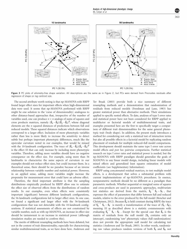
Figure 3 PC plots of allometry-free shape variation. All descriptions are the same as in Figure 2, but PCs were derived from Procrustes residuals after

regression of shape on log centroid size.

Analysis of high-dimensional phenotypic changeML Collyer et al

363

Heredity

accounting for the established coefficients in Br. Thus, randomizingraw phenotypic values does not preserve reduced model effects and is,therefore, not commensurate with the paradigm used by parametricMANOVA methods. As shown in the Supplementary Information,this can have devastating consequences for inferences made. Unawareacceptance of default probability distribution generation by np-MANOVA software is a likely reason for analytical malfeasance. Atthe time of this analysis, for example, the default setting for the adonisfunction in the vegan package (version 2.0.10) for R is a fullrandomization of raw data, advocated as having better ‘small samplecharacteristics’ (Oksanen et al., 2013). However, stratified resamplingis possible in this program, which means randomizing vectors ofvalues within strata. For example, male and female phenotypes can berandomized within populations. Stratified resampling is an obvioussolution to multifactor models without interactions. Performingnp-MANOVA with RRPP on sequential models extends the conceptof stratified resampling to factor or factor–covariate interactions, andalleviates the concern of inflated type I error rates because ofimproper sampling distributions based on suboptimal null models(Anderson and Legendre, 1999; Anderson, 2001b).

The important work of Anderson (2001a) introduced a method ofnp-MANOVA based on distance-based metrics and pseudometrics toaccommodate multivariate data in which Euclidean distances amongobservations might not be appropriate (that is, when response dataare not necessarily continuous). A link between distance-basedapproaches and MANOVA was established using linear modelsapplied to scores of principal coordinates analysis (Gower, 1966)based on appropriate principal coordinates (McArdle and Anderson,2001). Therefore, np-MANOVA using RRPP is possible with non-Euclidean distance-based characterization of disparity among obser-vations, by using either principal coordinates analysis or nonmetricmultidimensional scaling as a method of data transformation. Inaddition, np-MANOVA with RRPP should be adaptable to linearmodels with mixed effects and generalized least squares coefficientestimation (see Supplementary Information). Provided one can assignlogical reduced and full models, RRPP produces ‘correct exchangeableunits’ under a null hypothesis (Anderson and Ter Braak, 2003). Theexamples in this article illustrate a paradigm for evaluating all modeleffects, but the methodology could be applied to specific effects onlyor suites of effects. Understanding the paradigm enables researchers tochoose any nested models they wish to compare.

Although np-MANOVA with RRPP is a methodological approachthat should be commensurate with pairwise non-Euclidean distancesestimated from, for example, count data or presence/absence data (forexample, via using principal coordinate scores as data; see McArdleand Anderson, 2001), we do not wish to advocate that this approachshould supersede other methodological approaches that offer poten-tially better statistical properties. For example, Warton et al. (2012)demonstrated that multivariate analyses based on pairwise distancesignores important mean–variance associations for count data, leadingto erroneous analytical results. In these cases, generalized linearmodels should be used. Methods for employing generalized linearmodels for high-dimensional data, especially ecological ‘abundance’data, have been developed (Warton, 2011). Currently, the R package,mvabund (Wang et al., 2012), offers options to use generalized linearmodels on high-dimensional data, plus choose from among severalresampling methods, including bootstrap resampling of residuals, forhypothesis tests (based on methods described by Davison andHinkley, 1997; chapters 6 and 7). Similarly, hypothesis tests usinggeneralized linear models offer some similar challenges to thosepresented in this article, namely, selecting an appropriate resampling

algorithm for factor interactions (Warton, 2011). Althoughnp-MANOVA with RRPP might seem intuitively adaptable togeneralized linear models, two constraints limit its feasibility. First,several definitions of ‘generalized’ residuals are possible undergeneralized linear models (Pierce and Schafer, 1986; Davison andHinkley, 1997). Second, the pseudovalues generated by RRPP mightpreclude parameter estimation in random permutations (for example,if they are not binary or integers). Research to explore the feasibilityand statistical power of using generalized residuals from reducedmodels to generate sampling distributions of test statistics of fullmodels—which produce appropriate pseudovalues—would be aninteresting future direction. Nonetheless, np-MANOVA with RRPPand the ‘model-based’ approach to multivariate analysis of abundancedata (Warton, 2011) are rather commensurate in their approaches togeneral linear models and generalized linear models, respectively, inthat both (1) offer solutions for statistical analysis of high-dimensional data by (2) using resampling algorithms with residuals.

We also do not wish to inadvertently suggest that becausenp-MANOVA with RRPP in not constrained by an n44p expectation,that it is a salvo for estimation error because of small sample sizes,non-multivariate normality or heteroscedasticity. One should notconfuse statistical issues with proper parameter estimation. Theparadigm presented here targets the former issue and not the latter.Warton et al. (2012) demonstrated that hapless use of pairwisedistance-based MANOVA (Anderson, 2001a, b) can lead to inferentialerrors if linear model assumptions (evaluation of normality andhomoscedasticity) are ignored. Diagnostic analyses performed on theexamples that we presented here (see Supplementary Information)suggest that the inferences should be made with caution.

The greater point we intended to make is that it is important toremember in quantifying and comparing phenotypic change amongdifferent groups that taking a simpler approach to accommodatestatistical limitations could mean compromising the description ofphenotype. Parametric degrees of freedom do not constrain naturalselection, so why should describing the phenotypic response tonatural selection be constrained? The evolutionary biologist who iswilling to allow a high-dimensional definition of phenotype is capableof making additional discoveries. In the examples we used, weexpected to find reduced sexual dimorphism in the marsh habitat,as predators would mediate body shape by causing similar ecologicalroles between males and females, namely, streamlined body shapeassociated with predator avoidance swimming behavior. Based on asimpler definition of body shape, we did not find this to be the case,although we did observe consistent sexual dimorphisms anddifferences between habitats. However, in our higher-dimensionaldefinition of body shape, we found the counterintuitive result ofgreater sexual dimorphism in the marsh habitat, associated withfemales having different head shapes based on opercular curvature.This finding did not obscure inferences we could make about therelative lengths of caudal regions between habitats or the tendency fordeeper-bodied shapes of males, but it reveals morphologicallyfascinating results we had not considered.

Having an analytical paradigm that is not constrained by variablenumber equips researchers studying phenotypic evolution with thecapacity to simultaneously consider both subtle and general aspects ofphenotypic change, and should have positive influence on the typesof questions that can be asked in evolutionary biology research.We presented examples using morphometric data that define multi-dimensional traits. These examples have obvious appeal to researchersin the various fields of evolutionary biology concerned with pheno-typic evolution. These examples should also highlight the use of

Analysis of high-dimensional phenotypic changeML Collyer et al

364

Heredity

factorial models that are common in quantitative genetics research(that is, to address genotype by environment interactions). Extendingnp-MANOVA and RRPP to models with generalized least squaresestimation of parameters (see Supplementary Information) permitsanalysis of high-dimensional phenotypic data using genetic covariancematrices, as is typical with ecological genetics and evolutionarygenetics research. However, we also expect that the fields ofcomparative genomics, functional genomics and proteomics will alsocontinue to benefit from development of analytical tools forcomparative analyses for high-dimensional data. Recent methodolo-gical developments have improved the ability to extend thegeneralized linear model to high-dimensional data (Warton, 2011;Warton et al., 2012), allowing for collective analysis of multiplenoncontinuous variables (for example, discrete of categoricalvariables). The methods introduced here enable collective analysisof multiple continuous variables, plus allow multiple effects infactorial models or factor–covariate interactions to be evaluated withproper null models. These commensurate research directions willhopefully spur a synthesis for the analysis of high-dimensional data,irrespective of variable type. In this synthesis, the inclusion of themost biological information possible for an organism might beembraced rather than discouraged because of statistical limitations,for as we have shown, inferential ability can be positively associatedwith the amount of biological information used.

DATA ARCHIVING

Data available from the Dryad Digital Repository: doi:10.5061/dryad.1p80f.

CONFLICT OF INTEREST

The authors declare no conflict of interest.

ACKNOWLEDGEMENTSThis research was supported by a Western Kentucky University Research and

Creative Activities Program award (no. 12-8032) to MLC, an NSF REU

(DBI 1004665) grant-funded research experience to DJS and NSF grant

DEB-1257287 to DCA. Photographs of fish specimens were collected from the

Museum of Southwestern Biology, University of New Mexico, Albuquerque,

NM. We thank A Snyder and T Turner for access to museum specimens and

support in data collection. Samples were collected from lots MSB 49238 and

MSB 43612. Acquisition of photographs was made possible with funding from

a Faculty Research Grant from Stephen F Austin State University to MLC. We

thank M Smith, M Hall and M Ernst for assistance in digitizing photographs.

Adams DC (2014). Quantifying and comparing phylogenetic evolutionary rates for shapeand other high-dimensional phenotypic data. Syst Biol 63: 166–177.

Adams DC (2014). A generalized K statistic for estimating phylogenetic signal from shapeand other high-dimensional multivariate data. Syst Biol 63: 685–697

Adams DC, Collyer ML (2007). Analysis of character divergence along environmentalgradients and other covariates. Evolution 61: 510–515.

Adams DC, Collyer ML (2009). A general framework for the analysis of phenotypictrajectories in evolutionary studies. Evolution 63: 1143–1154.

Adams DC, Felice R (2014). Assessing phylogenetic morphological integration and traitcovariation in morphometric data using evolutionary covariance matrices. PLoS ONE 9:e94335.

Adams DC, Otarola-Castillo E (2013). An R package for the collection and analysis ofgeometric morphometric shape data. Methods Ecol Evol 4: 393–399.

Adams DC, Collyer ML, Otarola-Castillo E, Sherratt E (2014). geomorph: Software forgeometric morphometric analyses. R package version 2.1. Available at http://CRAN.R-project.org/package=geomorph.

Adams DC, Rohlf FJ, Slice DE (2013). A field comes of age: geometric morphometrics inthe 21st century. Hystrix 24: 7–14.

Anderson MJ (2001a). A new method for non-parametric multivariate analysis of variance.Aust Ecol 26: 32–46.

Anderson MJ (2001b). Permutation tests for univariate or multivariate analysis of varianceand regression. Can J Fish Aquat Sci 58: 626–639.

Anderson MJ, Legendre P (1999). An empirical comparison of permutation methodsfor tests of partial regression coefficients in a linear model. J Stat Comput Simul62: 271–303.

Anderson MJ, Ter Braak CJF (2003). Permutation tests for multi-factorial analysis ofvariance. J Stat Comput Simul 73: 85–113.

Arnold SJ (2005). The ultimate causes of phenotypic integration: lost in translation.Evolution 59: 2059–2061.

Blows MW (2007). A tale of two matrices: multivariate approaches in evolutionary biology.J Evol Biol 20: 1–8.

Bookstein FL (1991). Morphometric Tools for Landmark Data: Geometry and Biology.Cambridge University Press: Cambridge.

Brodie ED, Moore AJ, Janzen FJ (1995). Visualizing and quantifying natural selection.Trends Ecol Evol 10: 313–318.

Collyer ML, Adams DC (2007). Analysis of two-state multivariate phenotypic change inecological studies. Ecology 88: 683–692.

Collyer ML, Adams DC (2013). Phenotypic trajectory analysis: comparison of shapechange patterns in ecology and evolution. Hystrix 24: 75–83.

Collyer ML, Heilveil JS, Stockwell CA (2011). Contemporary evolutionary divergence for aprotected species following assisted colonization. PLoS ONE 6: e22310.

Collyer ML, Novak JM, Stockwell CA (2005). Morphological divergence of native and recentlyestablished populations of White Sands Pupfish (Cyprinodon tularosa). Copeia 2005:1–11.

Collyer ML, Stockwell CA, Dean CA, Reiser MH (2007). Phenotypic plasticity andcontemporary evolution in introduced populations: Evidence from translocatedpopulations of white sands pupfish (Cyrpinodon tularosa). Ecol Res 22: 902–910.

Davison AC, Hinkley DV (1997). Bootstrap Methods and their Application (CambridgeSeries in Statistical and Probabilistic Mathematics). Cambridge University Press:Cambridge.

Freedman D, Lane D (1983). A nonstochastic interpretation of reported significance levels.J Bus Econ Stat 1: 292–298.

Goodall CR (1991). Procrustes methods in the statistical analysis of shape. J R Stat Soc BMethodoll 53: 285–339.

Gower JC (1966). Some distance properties of latent rootand vector methods used inmultivariate analysis. Biometrika 53: 325–338.

Huttegger SM, Mitteroecker P (2011). Invariance and meaningfulness in phenotypespaces. Evol Biol 38: 335–351.

Klingenberg CP, Gidaszewski NA (2010). Testing and quantifying phylogenetic signals andhomoplasy in morphometric data. Syst Biol 59: 245–261.

Lande R (1979). Quantitative genetic analysis of multivariate evolution, applied to brain:body size allometry. Evolution 33: 402–416.

Lande R (1980). Sexual dimorphism, sexual selection, and adaptation in polygeniccharacters. Evolution 34: 292–305.

Lande R (1981). Models of speciation by sexual selection on polygenic traits. Proc NatlAcad Sci USA 78: 3721–3725.

Lande R, Arnold SJ (1983). The measurement of selection on correlated characters.Evolution 37: 1210–1226.

Langerhans RB, Layman CA, Shokrollahi AM, DeWitt TJ (2004). Predator-drivenphenotypic diversification in Gambusia affinis. Evolution 58: 2305–2318.

McArdle BH, Anderson MJ (2001). Fitting multivariate models to community data:a comment on distance-based redundancy analysis. Ecology 82: 290–297.

Oksanen J, Blanchet FG, Kindt R, Legendre P, Minchin PR, O’Hara RB et al. (2013).vegan: Community ecology package. R package version 2.0-10. Available at http://CRAN.R-project.org/package=vegan.

Phillips PC, Arnold SJ (1989). Visualizing multivariate selection. Evolution 43:1209–1222.

Pierce DA, Schafer DW (1986). Residuals in generalized linear models. J Am Stat Assoc81: 977–986.

R Core Team (2014). R Foundation for Statistical Computing. Vienna, Austria.Rencher AC, Christensen WF (2012). Methods of Multivariate Analysis, 3rd Edition. John

Wiley & Sons, Inc.: Hoboken, NJ.Rohlf FJ, Corti M (2000). Use of two-block partial least-squares to study covariation in

shape. Syst Biol 49: 740–753.Rohlf FJ, Marcus LF (1993). A revolution in morphometrics. Trends Ecol Evol 8: 129–132.Rohlf FJ, Slice D (1990). Extensions of the Procrustes method for the optimal super-

imposition of landmarks. Syst Zool 39: 40–59.Schluter D (2000). The Ecology of Adaptive Radiation. Oxford University Press: Oxford, UK.Shaw RG, Mitchell-Olds T (1993). ANOVA for unbalanced data: an overview. Ecology 74:

1638–1645.Wang Y, Naumann U, Wright ST, Warton DI (2012). mvabund- an R package for model-

based analysis of multivariate abundance data. Methods Ecol Evol 3: 471–474.Warton DI (2011). Regularized sandwich estimators for analysis of high-dimensional data

using generalized estimating equations. Biometrics 67: 116–123.Warton DI, Wright ST, Wang Y (2012). Distance-based multivariate analyses confound

location and dispersion effects. Methods Ecol Evol 3: 89–101.

Supplementary Information accompanies this paper on Heredity website (http://www.nature.com/hdy)

Analysis of high-dimensional phenotypic changeML Collyer et al

365

Heredity