A Memetic Algorithm for the Green Vehicle Routing Problem

sustainability

Article

A Memetic Algorithm for the Green VehicleRouting Problem

Bo Peng 1, Yuan Zhang 1, Yuvraj Gajpal 2 and Xiding Chen 3,*1 School of Business Administration, Southwestern University of Finance and Economics,

Chengdu 610074, China; [email protected] (B.P.); [email protected] (Y.Z.)2 Asper School of Business, University of Manitoba, Winnipeg, MB R3T 5V4, Canada;

[email protected] Department of Finance, Wenzhou Business College, Wenzhou, 325035, China* Correspondence: [email protected]

Received: 17 August 2019; Accepted: 15 October 2019; Published: 31 October 2019��

Abstract: The green vehicle routing problem is a variation of the classic vehicle routing problem inwhich the transportation fleet is composed of electric vehicles with limited autonomy in need ofrecharge during their duties. As an NP-hard problem, this problem is very difficult to solve. In thispaper, we first propose a memetic algorithm (MA)—a population-based algorithm—to tackle thisproblem. To be more specific, we incorporate an adaptive local search procedure based on a rewardand punishment mechanism inspired by reinforcement learning to effectively manage the multipleneighborhood moves and guide the search, an effective backbone-based crossover operator to generatethe feasible child solutions to obtain a better trade-off between intensification and diversification ofthe search, and a longest common subsequence-based population updating strategy to effectivelymanage the population. The purpose of this research is to propose a highly effective heuristic forsolving the green vehicle routing problem and bring new ideas for this type of problem. Experimentalresults show that our algorithm is highly effective in comparison with the current state-of-the-artalgorithms. In particular, our algorithm is able to find the best solutions for 84 out of the 92 instances.Key component of the approach is analyzed to evaluate its impact on the proposed algorithm and toidentify the appropriate search mechanism for this type of problem.

Keywords: green vehicle routing problem; memetic algorithm; adaptive local search; crossoveroperator

1. Introduction

Currently, environmental concerns have driven governments to develop regulations and lawsthat require organizations to adopt green logistics methods in their operations [1]. As a result, majorautomotive manufacturers design and produce increasingly more and better alternative fuel vehicles(AFVs). Hence, the number of AFVs on the roads are increasing. AFVs represent a promisingopportunity for reducing costs and pollution caused by transportation and mobility operations [2].This is because many AFV models in the market not only help reduce fuel consumption, but alsohave advantages in reducing fuel costs and reducing greenhouse gas emissions. However, manyAFVs have limited travel distances and must often rely on an underdeveloped refueling infrastructure.Therefore, it may be necessary to include the exact locations of the refueling stations in route planning.Furthermore, refueling delays may also cause considerable negative impacts. For example, for electricvehicles, due to their relatively short driving range and long recharging time, coupled with limitedcharging infrastructure, it may lead to range anxiety, so consumers may be worried about insufficient

Sustainability 2019, 11, 6055; doi:10.3390/su11216055 www.mdpi.com/journal/sustainability

http://www.mdpi.com/journal/sustainability

http://www.mdpi.com

https://orcid.org/0000-0002-7105-8926

https://orcid.org/0000-0001-7801-2261

http://www.mdpi.com/2071-1050/11/21/6055?type=check_update&version=1

http://dx.doi.org/10.3390/su11216055

http://www.mdpi.com/journal/sustainability

Sustainability 2019, 11, 6055 2 of 20

energy to reach the desired destination [3]. As a result, new routing models and methods for AFVshave emerged to help provide reliable and adequate levels of service.

As one of the most famous combinatorial optimization problems, the classic vehicle routingproblem (VRP) is concerned with designing least cost delivery routes for a fleet of vehicles to serve aset of customers. The green vehicle routing problem (GVRP) is a variation of the classic VRP in whichthe fleet is composed of alternative fuel powered vehicles with limited autonomy in need of rechargeduring the execution of their duties [4]. For the GVRP, there is an unlimited homogeneous fleet ofalternative fuel vehicles with limited time that starts from a depot node 0 and returns to it with theobjective of minimizing the total travel distances incurred by all the vehicles. The vehicles must fulfillall the requests by visiting each customer node once with the constraints on the maximum drivingtime and maximum fuel capacity available [5]. Figure 1 depicts a feasible solution to a green VRP.

Sustainability 2019, 11, x FOR PEER REVIEW 2 of 22

As one of the most famous combinatorial optimization problems, the classic vehicle routing problem (VRP) is concerned with designing least cost delivery routes for a fleet of vehicles to serve a set of customers. The green vehicle routing problem (GVRP) is a variation of the classic VRP in which the fleet is composed of alternative fuel powered vehicles with limited autonomy in need of recharge during the execution of their duties [4]. For the GVRP, there is an unlimited homogeneous fleet of alternative fuel vehicles with limited time that starts from a depot node 0 and returns to it with the objective of minimizing the total travel distances incurred by all the vehicles. The vehicles must fulfill all the requests by visiting each customer node once with the constraints on the maximum driving time and maximum fuel capacity available [5]. Figure 1 depicts a feasible solution to a green VRP.

Figure 1. Example of a feasible solution for green VRP.

The goal of this research is to propose a highly effective heuristic for solving the green vehicle routing problem and to bring new ideas for this problem or this type of problem. The main contributions of this paper can be summarized as follows. First, to the best of our knowledge, this work is the first to employ a population-based algorithm (i.e., memetic algorithm (MA)) to solve the green vehicle routing problem. Second, we propose a reward and punishment mechanism inspired by reinforcement learning to effectively manage the multiple neighborhood moves and guide the search. Compared with the traditional local search, the adaptive local search can manage the different neighborhood moves to adapt to different instances. Third, a backbone-based crossover operator and a longest common subsequence based (LCS-based) population updating strategy is devised to obtain a better trade-off between intensification and diversification of the search. Compared to the general crossover operator (such as one-point crossover operator), the backbone-based crossover operator can better integrate with the problem structure by inheriting the promising customer and station sequences from the routes. Fourth, our experimental results demonstrate that the performance of our MA is highly effective compared to state-of-the-art approaches in the literature.

The rest of the paper is organized as follows. In Section 2, we present the review of the literature. In Section 3, we give the problem description of GVRP. In Section 4, we provide details of our memetic algorithm. In Section 5, we present the results of extensive computational experiments carried out to assess the performance of the proposed algorithms in comparison to current best-performing approaches. In Section 6, we analyze the important component (i.e., adaptive mechanism for neighborhood moves) of the MA algorithm and study the impact on its performance. In Section 7, we discuss the proposed algorithm in comparison with the other methods in the literature. Finally, we provide concluding remarks as well as potential research directions in Section 8.

2. Review of the Literature

Figure 1. Example of a feasible solution for green VRP.

The goal of this research is to propose a highly effective heuristic for solving the green vehiclerouting problem and to bring new ideas for this problem or this type of problem. The main contributionsof this paper can be summarized as follows. First, to the best of our knowledge, this work is the firstto employ a population-based algorithm (i.e., memetic algorithm (MA)) to solve the green vehiclerouting problem. Second, we propose a reward and punishment mechanism inspired by reinforcementlearning to effectively manage the multiple neighborhood moves and guide the search. Comparedwith the traditional local search, the adaptive local search can manage the different neighborhoodmoves to adapt to different instances. Third, a backbone-based crossover operator and a longestcommon subsequence based (LCS-based) population updating strategy is devised to obtain a bettertrade-off between intensification and diversification of the search. Compared to the general crossoveroperator (such as one-point crossover operator), the backbone-based crossover operator can betterintegrate with the problem structure by inheriting the promising customer and station sequences fromthe routes. Fourth, our experimental results demonstrate that the performance of our MA is highlyeffective compared to state-of-the-art approaches in the literature.

The rest of the paper is organized as follows. In Section 2, we present the review of the literature.In Section 3, we give the problem description of GVRP. In Section 4, we provide details of our memeticalgorithm. In Section 5, we present the results of extensive computational experiments carried out toassess the performance of the proposed algorithms in comparison to current best-performing approaches.In Section 6, we analyze the important component (i.e., adaptive mechanism for neighborhood moves)of the MA algorithm and study the impact on its performance. In Section 7, we discuss the proposed


algorithm in comparison with the other methods in the literature. Finally, we provide concludingremarks as well as potential research directions in Section 8.

2. Review of the Literature

The green vehicle routing problem was first introduced in [6], where a mixed integer linearprogramming formulation and two heuristics are proposed. One of the proposed heuristics is amodified Clarke and Wright savings algorithm (MCWS) that repairs infeasible routes by inserting fuelvehicle stations (AFSs) using a savings criterion and removes redundant AFSs after merging the routes.

Schneider et al. (2014) [7] introduced the electric vehicle routing problem with time windowsand recharging stations (E-VRPTW), which is an extension of the VRP with a fleet of electric vehicles.The E-VRPTW problem considers limited capacities of vehicles, time windows of customers, andthe possibility of recharging at any of the available stations using an appropriate recharging scheme.For this problem, they proposed an MILP formulation and a hybrid metaheuristic combining variableneighborhood search and tabu search (VNS/TS). The proposed VNS/TS explores infeasible solutionswith respect to capacity, time windows, and battery usage constraints. A dynamic penalizing schemeis used to guide the search toward feasible solutions. Furthermore, Schneider et al. (2014) [7] madeimprovement over the MILP formulation proposed by Erdogan and Miller-Hooks (2012) [6], andthey evaluated their VNS/TS and MILP approaches on the 52 instances proposed by Erdogan andMiller-Hooks (2012) [6]. Computational experiments showed that CPLEX 12.2 was unable to solveto optimality instances with 20 customers using their MILP model, and VNS/TS outperformed theconstructive heuristics proposed by Erdogan and Miller-Hooks (2012) [6]. Schneider et al. (2015) [8]introduced the vehicle routing problem with intermediate stops (VRPIS) that generalizes the GVRP andthe MDVRPI. To solve this problem, they proposed an adaptive variable neighborhood search (AVNS).Their AVNS uses a modified savings algorithm to generate an initial solution that is later improvedwith local search. The algorithm uses an adaptive shaking with 24 neighborhood structures, five routeselection methods, three vertex sequence selection methods, and an adaptive mechanism to choosethe route and vertex selection methods. The solution generated at the shaking step is subsequentlyimproved by several greedy local searches. Furthermore, the AVNS has a dynamic penalization schemeto guide the search toward feasible solutions and a simulated annealing acceptance criterion. Since thegreen VRP is a special case of the VRPIS, Schneider et al. (2015) [8] evaluated their approach on theinstances of Erdogan and Miller-Hooks (2012) [6]. This method outperformed all previous methodsboth in terms of solution quality and computational time.

More recently, Montoya et al. (2016) [5] presented a new mathematical formulation for the GVRPand a branch-and-cut algorithm. The authors also proposed a simulated annealing heuristic andreport results on small instances with up to 20 customers and 310 refueling stations. Andelmin andBartolini (2019) [1] proposed a multi-start local search (MSLS) algorithm for the GVRP. Their MSLSalgorithm consists of three phases. The first two phases iteratively construct new solutions, improvethem by local search, and store all vehicle routes from these solutions in a route pool. The thirdphase optimally combines vehicle routes in the route pool by solving a set partitioning problemand improves the final solution by local search. They reported computational results on benchmarkinstances with up to 470 customers, showing that the algorithm is highly competitive with the previousbest performing heuristics.

Swarm intelligence (SI) is the collective behavior of decentralized and self-organized systems,natural or artificial. The concept is employed in work on artificial intelligence. This method iswidely employed to solve hard solving complex combinatorial decision problems [9–12]. As a typeof evolutionary algorithm [3], memetic algorithm is a general-purpose metaheuristic approach thattypically combines a local search optimization procedure with a population-based framework. Memeticalgorithm has been successfully applied to tackle many classical combinatorial optimization problems,including the machine scheduling problem [13], graph coloring problem [14] and quadratic assignment


problem [15]. Hence, in this paper, we first employ the memetic algorithm to tackle the famous greenvehicle routing problem.

3. Problem Description and Definitions

Problem Description

For the green vehicle routing problem, the objective is to find a set of routes of minimum totaldistance such that each customer is visited exactly once; the level of the tank when the vehicle arrivesat any vertex is nonnegative; each route satisfies the maximum-duration limit; and each route startsand ends at the depot. Figure 1 depicts a feasible solution to a green VRP.

More precisely, we are given a set N = {1, . . . , n} of n customers and a set of F = {n + 1, . . . , n + s}of s refueling stations. There is an unlimited homogeneous fleet of alternative fuel vehicles withlimited time that starts from a depot node 0 and return to it with the objective of minimizing the totaltravel distances incurred by all the vehicles. The vehicles must fulfill all the requests by visiting eachcustomer node once with the constraints on the maximum driving time and maximum fuel capacityavailable. More precisely, GVRP can be defined on a complete weighted undirected graph G = (V, E)with the following features.

V = N ∪ F ∪ 0 denotes the set of nodes, where N denotes the set of customer nodes, F isthe set of refueling station nodes, 0 denotes the starting and ending node, also called depot, andE = {(u, v): u, v∈V, u,v} is the edge set.

The distance between two nodes (u, v ∈ N) is denoted by c(u, v).

• The service time at each customer node u ∈ N is denoted by stu.• The refueling time at each refueling station node u ∈ F is denoted by f tu.• The travel time to traverse the arc (u, v) ∈ E is denoted by ttu,v.• The maximum fuel capacity without refueling for each vehicle is MC (i.e., the maximum fuel

capacity constraint).• The maximum driving time of each route including the service time, traversal time and refueling

time is MT (i.e., the maximum driving time constraint).• A route traveling from i to j consumes c(i, j) units of distance and t(i, j) units of time. The time t(i, j)

is assumed to be proportional to the distance c(i, j) from i to j and computed as t(i, j) = c(i, j)/vwhere v is the vehicle speed.

Let R be one route in a solution S and R = {u0 = 0, u1, u2, . . . , um−1, um = 0}, where uk is the kthnode visited in R(0 ≤ k ≤ m). It is worth noting that the GVRP expresses the maximum driving rangeof a vehicle as its maximum fuel capacity MC. However, since vehicle fuel consumption is assumedto be linearly dependent on the distance traveled, the maximum driving range can be equivalentlyexpressed as a distance value. Letting K be the constant rate of fuel consumption per distance unit, themaximum distance Q that a vehicle can travel without refueling is thus defined as Q = MC/K.

If the visited node is a customer node (i.e., uk ∈ N), the corresponding fuel surplus of the vehicleafter visiting it is f s(uk) = f s(uk−1) − c(uk−1, uk)/K. For each node in the route, the correspondingfuel surplus must be non-negative. Note that all vehicles departing from the depot and the refuelstations are assumed to be fully refueled having the maximum fuel amount MC. We denote byDT(R) =

∑m−1k=0 ttuk,uk+1 the total traversal time, ST(R) =

∑m−1k=1 stuk the total service time if uk is the

customer node, and FT(R) =∑m−1

k=1 f tuk if uk is the refuel station node. The corresponding totalduration of each route including the traversal time, service time and refuel time cannot exceed the givenmaximum driving time, i.e., DT(R) + ST(R) + FT(R) ≤ MD(the maximum driving time constraint).The objective is to find a feasible solution with the minimum total travel distance as follows:

Minimize f (s) =∑|S|

i=1DT(R i) ∗ v, (1)


where DT denotes the traversal time and v denotes the vehicle speed.

4. Memetic Algorithm

4.1. Main Framework

A memetic algorithm is a general-purpose metaheuristic approach that typically combines a localsearch optimization procedure with a population based framework, which has been successfully appliedto tackle many classical combinatorial optimization problems, including the job shop schedulingproblem [16], p-center problem [17] and nurse rostering problem [18]. The purpose of combininglocal search and population-based strategies is to take advantage of both the crossover operator asa diversification mechanism for discovering promising unexplored regions of the search space andthe local optimization as an intensification procedure to obtain high quality solutions within a searchregion. We outline our proposed memetic algorithm for GVRP in Algorithm 1. At the beginning of thealgorithm, we iteratively employ a hybrid heuristic method to generate the initial population (line 1).Following this, we employ an adaptive local search to optimize the solutions in the population (lines2–4). Later, we iteratively combine two parent solutions randomly selected from the population togenerate offspring solutions using a backbone-based crossover operator until the stopping criterion,i.e., maximum computing time, is satisfied (lines 5–7). After each use of the crossover operator,we improve the generated offspring solution using an adaptive local search to guide the search topromising regions (line 8). During this process, S∗ records the best solution found so far (lines 9–11).We then apply the longest-common-sequence-based (LCS-based) population updating strategy topossibly replace the worst individual in the population with the improved offspring solution (lines12–15).

Algorithm 1. Framework of the memetic algorithm for solving GVRP

Require: Benchmark instance (B); the maximum computing time (Tmax)Ensure: Best-found solution (S∗)/* Generate np feasible solutions as an initial population (Section 4.2) */1: Pc =

{S1, . . . , Snp

}← Initial solutions (B)

/* Improve each individual Si in the population with an adaptive local search (Section 4.3) */2: for i = 1, . . . , np do3: Si ← Adaptive local search (Si)4: end for5: while the maximum computing time Tmax is not reached do6: Randomly select parent solutions Si and S j, from P where 1 ≤ i, j ≤ np an i , j/* Generate offspring Sc from Si, and S j, (Section 4.4) */7: Sc ← Si ⊕ S j = Backbone-based-crossover (Si, S j)/* Improve Sc with an adaptive local search (Section 4.3) */8: Sc ← Adaptive-local-search (Sc)9: if Sc is better than S∗ then10: S∗ ← Sc

11: end if/* The longest-common-subsequence based population updating strategy (Section 4.5) */12: Determine the worst individual Sw where the goodness value GS(Sw, Pc) = min

{GS(Sk, Pc)

}, 1 ≤ k ≤ np

(see Equation (7))13: if GS(Sc, Pc ∪ Sc) > GS(Sw, Pc ∪ Sc) then14: Pc ← Pc ∪ Sc\Sw

15: end if16: end while17: return (S∗)


4.2. Initial Solutions

In this section, we employ a constructive heuristic based on a greedy generation method calledk-Pseudo Greedy proposed by Felipe et al. (2014) [2] to generate the initial population. The k-PseudoGreedy focuses more on feasibility and diversification, producing multiple different feasible solutions,rather than on quality or cost that are to be improved later. Specifically, the k-Pseudo Greedy methodcreates feasible solutions by starting from an empty solution and iteratively extending it (i.e., addingcustomers and fuel stations in route) until a complete solution is constructed. Specifically, the methodfirst finds up to k unvisited customers that are closest to the current node and are reachable accordingto capacity, autonomy and time availability, and then select one of them, denoted by j, at random.More precisely, if it is possible to reach the depot directly form j, then j is added to the initial route.If it is possible to reach the depot from j by visiting a recharge node r, the j and r are both added to theinitial route. Otherwise, the current route is ended in depot. The above procedure iteratively continuesuntil all the customers are added in the initial solution.

If k = 1, it reduces to a nearest neighbor greedy algorithm, visiting the closest customer andrecharging at the closest recharge station when needed, until the capacity or time limit is reached.If k > 1, the next node to be visited is chosen randomly from the set of k closest candidates, allowing thegeneration of different feasible solutions in different runs. This algorithm is focused more on feasibilityand diversification, producing multiple different feasible solutions, rather than on quality or cost,that are to be improved later. However, if k is small, the produced solutions are expected to have anacceptable quality.

Generally speaking, the initial solution procedure will have an insignificant impact on theperformance of the overall algorithm, if the algorithm itself is powerful enough. Therefore, we adoptin this study this simple but effective initial solution construction process above to generate theinitial population.

4.3. Adaptive Local Search

One of the key components of our memetic algorithm is the adaptive local search procedure thatplays the critical role of intensifying the search. With the exception of tabu search, traditional localsearch utilizes a set of moves to search the solution regions without maintaining a memory of theprocess, while the local search based on our reinforcement learning mechanism is able to effectivelyexploit memory to manage the neighborhood moves and guide the search to promising regions.

4.3.1. Neighborhood Moves

Our algorithm employs both intra-route moves (performed in the same route) and inter-routemoves (performed between two different routes) as follows:

• Intra-node-insertion (hereafter denoted as M1): This operator selects a customer node removedfrom a given route and tries to relocate it in the same route. Specifically, it first removes node iand relocates it between customers k and l to contains the customer sequence (k, i, l), as shown inFigure 2.

• Intra-nodes-swap (M2): two customer nodes in the same route exchange their positions. Specifically,it first removes nodes i and k and relocates them in the current route to contains the customersequences (AFS1, k, j) and (AFS2, i, l), as shown in Figure 3.

• Intra-arc-insertion (M3): this operator selects an arc of two customers from a given route and triesto relocate it somewhere else of the same route. Specifically, it first removes one arc between twosuccessive customers i and j. It then tries to reconnect the route so that it contains the customersequence (AFS2, k, j, 0), as shown in Figure 4.

• Intra-arcs-swap (M4): two arcs of consecutive customers exchange their positions. See an exampleshown in Figure 5.


• Inter-node-insertion (M5): different from the intra-node-insertion operator, this operator selectsa customer node removed from a given route and tries to relocate it in a different route. To bespecific, it first removes node i in route 1 and relocates it between customers k and l to containsthe customer sequence (k, i, l) in route 2, as shown in Figure 6.

• Inter-nodes-swap (M6): different from the intra-nodes-swap, this operator selects two customersin different routes to exchange their positions. See an example in Figure 7.

• Inter-arc-insertion (M7): different from the intra-arc-insertion operator, this operator relocates acustomer arc into another route. See an example in Figure 8.

• Inter-arcs-swap (M8): different from the intra-arcs-swap operator, this operator exchanges thepositions of two customer arcs between two different routes. See an example in Figure 9.


(a) (b)

Figure 2. Example of the intra-node-insertion operator relocating customer node i of the current route between customers k and l.

• Intra-nodes-swap ( 2M ): two customer nodes in the same route exchange their positions.

Specifically, it first removes nodes i and k and relocates them in the current route to contains the customer sequences 1( , , )AFS k j and 2( , , )AFS i l , as shown in Figure 3.

(a) (b)

Figure 3. Example of the intra-nodes-swap operator relocating customer node i of the current route between refuel station AFS2 and customer l, and relocating customer node k of the current route between refuel station AFS2 and customer l.

• Intra-arc-insertion ( 3M ): this operator selects an arc of two customers from a given route and tries to relocate it somewhere else of the same route. Specifically, it first removes one arc between two successive customers i and j. It then tries to reconnect the route so that it contains the customer sequence 2( , , , 0)AFS k j , as shown in Figure 4.

(a) (b)

Figure 4. Example of the intra-arc-insertion operator relocating customer arc (i, j) of the current route between refuel station AFS2 and depot 0.

• Intra-arcs-swap ( 4M ): two arcs of consecutive customers exchange their positions. See an example shown in Figure 5.

Figure 2. Example of the intra-node-insertion operator relocating customer node i of the current routebetween customers k and l.


(a) (b)




(a) (b)



(a) (b)



Figure 3. Example of the intra-nodes-swap operator relocating customer node i of the current routebetween refuel station AFS2 and customer l, and relocating customer node k of the current routebetween refuel station AFS2 and customer l.


(a) (b)




(a) (b)



(a) (b)



Figure 4. Example of the intra-arc-insertion operator relocating customer arc (i, j) of the current routebetween refuel station AFS2 and depot 0.

Sustainability 2019, 11, 6055 8 of 20Sustainability 2019, 11, x FOR PEER REVIEW 8 of 22

(a) (b)

Figure 5. Example of the intra-arcs-swap operator relocating customer arc (i, j) of the current route between refuel stations AFS2 and AFS3 and relocating customer arc (k, l) of the current route between refuel stations AFS1 and AFS2.

• Inter-node-insertion ( 5M ): different from the intra-node-insertion operator, this operator selects a customer node removed from a given route and tries to relocate it in a different route. To be specific, it first removes node i in route 1 and relocates it between customers k and l to contains the customer sequence ( , , )k i l in route 2, as shown in Figure 6.

(a) (b)

Figure 6. Example of the inter-node-insertion operator relocating customer i of route 1 into route 2 between customer k and l.

• Inter-nodes-swap ( 6M ): different from the intra-nodes-swap, this operator selects two customers in different routes to exchange their positions. See an example in Figure 7.

(a) (b)

Figure 7. Example of the inter-nodes-swap operator swapping the positions of customers i and k in route 1 and route 2, respectively.

• Inter-arc-insertion ( 7M ): different from the intra-arc-insertion operator, this operator relocates a customer arc into another route. See an example in Figure 8.

Figure 5. Example of the intra-arcs-swap operator relocating customer arc (i, j) of the current routebetween refuel stations AFS2 and AFS3 and relocating customer arc (k, l) of the current route betweenrefuel stations AFS1 and AFS2.


(a) (b)



(a) (b)



(a) (b)



Figure 6. Example of the inter-node-insertion operator relocating customer i of route 1 into route 2between customer k and l.


(a) (b)



(a) (b)



(a) (b)



Figure 7. Example of the inter-nodes-swap operator swapping the positions of customers i and k inroute 1 and route 2, respectively.Sustainability 2019, 11, x FOR PEER REVIEW 9 of 22

(a) (b)

Figure 8. Example of the inter-arc-insertion operator relocating customer arc ( , )i j of route 1 into

route 2 between depot 0 and customer s.

• Inter-arcs-swap ( 8M ): different from the intra-arcs-swap operator, this operator exchanges the positions of two customer arcs between two different routes. See an example in Figure 9.

Figure 9. Example of the inter-arcs-swap operator swapping the positions of customer arc (i, j) in route 1 and customer arc (s, t) in route 2.

In our local search, we only consider neighborhood moves that can satisfy both two constraints, i.e., the maximum driving time, and maximum fuel capacity constraints.

4.3.2. Reward and Penalty Strategy Based on Adaptive Mechanism

Reinforcement learning is an area of machine learning concerned with how an agent should take actions in an environment to maximize cumulative reward. The intuition underlying reinforcement learning is that actions that lead to large rewards should be made more likely to recur.

We employ a reward and penalty strategy to dynamically manage the neighborhood moves and guide the search based on the expectation that different neighborhood moves may be preferable for different problem instances or search landscapes. Consequently, we keep track of a score for each neighborhood move, which measures how well the move has performed for the current instance or landscape, adopting the perspective that alternating among different moves based on the proposed adaptive mechanism may yield more robust performance.

To select moves, we assign scores to different moves and use the roulette wheel selection principle. If we haven moves with scores ( )1,2,...,isc i n∈ , move k is selected with probability

kλ , where

1,

nk

ki i

scsc

λ=

= 1, 2,..., .k n= (2)

At the beginning of the search, each neighborhood move has the same score 0sc and hence the same probability of being chosen. After each iteration j , the score of the neighborhood used is updated as follows:

Figure 8. Example of the inter-arc-insertion operator relocating customer arc (i, j) of route 1 into route2 between depot 0 and customer s.



(a) (b)

Figure 8. Example of the inter-arc-insertion operator relocating customer arc ( , )i j of route 1 into

route 2 between depot 0 and customer s.

• Inter-arcs-swap ( 8M ): different from the intra-arcs-swap operator, this operator exchanges the positions of two customer arcs between two different routes. See an example in Figure 9.

Figure 9. Example of the inter-arcs-swap operator swapping the positions of customer arc (i, j) in route 1 and customer arc (s, t) in route 2.

In our local search, we only consider neighborhood moves that can satisfy both two constraints, i.e., the maximum driving time, and maximum fuel capacity constraints.


Reinforcement learning is an area of machine learning concerned with how an agent should take actions in an environment to maximize cumulative reward. The intuition underlying reinforcement learning is that actions that lead to large rewards should be made more likely to recur.

We employ a reward and penalty strategy to dynamically manage the neighborhood moves and guide the search based on the expectation that different neighborhood moves may be preferable for different problem instances or search landscapes. Consequently, we keep track of a score for each neighborhood move, which measures how well the move has performed for the current instance or landscape, adopting the perspective that alternating among different moves based on the proposed adaptive mechanism may yield more robust performance.

To select moves, we assign scores to different moves and use the roulette wheel selection principle. If we haven moves with scores ( )1,2,...,isc i n∈ , move k is selected with probability

kλ , where

1,

nk

ki i

scsc

λ=

= 1, 2,..., .k n= (2)

At the beginning of the search, each neighborhood move has the same score 0sc and hence the same probability of being chosen. After each iteration j , the score of the neighborhood used is updated as follows:

Figure 9. Example of the inter-arcs-swap operator swapping the positions of customer arc (i, j) in route1 and customer arc (s, t) in route 2.

In our local search, we only consider neighborhood moves that can satisfy both two constraints,i.e., the maximum driving time, and maximum fuel capacity constraints.


Reinforcement learning is an area of machine learning concerned with how an agent should takeactions in an environment to maximize cumulative reward. The intuition underlying reinforcementlearning is that actions that lead to large rewards should be made more likely to recur.

We employ a reward and penalty strategy to dynamically manage the neighborhood moves andguide the search based on the expectation that different neighborhood moves may be preferable fordifferent problem instances or search landscapes. Consequently, we keep track of a score for eachneighborhood move, which measures how well the move has performed for the current instance orlandscape, adopting the perspective that alternating among different moves based on the proposedadaptive mechanism may yield more robust performance.

To select moves, we assign scores to different moves and use the roulette wheel selection principle.If we have n moves with scores sci(i ∈ 1, 2, . . . , n), move k is selected with probability λk, where

λk =n∑

i=1

scksci

,k = 1, 2, . . . , n. (2)

At the beginning of the search, each neighborhood move has the same score sc0 and hence thesame probability of being chosen. After each iteration j, the score of the neighborhood used is updatedas follows:

sci, j+1 = sci, j + α ∗ βl, i, j = 1, 2, . . . , n; l = 1, 2. (3)

where the reaction factor α controls how quickly the score adjustment function reacts to changesaccording to the performance of the moves, and parameter β denotes the different incremental scoresaccording to the following several situations. If one move can produce a new best solution, we rewardthis neighborhood move by choosing β1 in Equation (3). If one move can generate a better solution thanthe current solution, the neighborhood move would still be rewarded β2. However, if the generatedsolution is worse than the current solution, then we punish the move by multiplying the score by γas follows:

sci, j+1 = γ ∗ sci, j, i, j = 1, 2, . . . , n. (4)

The adaptive local search phase proceeds with iterative exploitation of the eight neighborhoodmoves as shown in Algorithm 2. In each iteration, one neighborhood move is picked with probability λi(lines 3–4). Then, if the neighborhood solution S’ obtained by this neighborhood move cannotimprove the current solution S, the next neighborhood move is chosen from those remaining;otherwise, the current solution S is replaced by the best neighborhood solution S′ generated bycurrent neighborhood move (lines 5–10). Subsequently, the score of the neighborhood move Ni isupdated by Equations (3) and (4) (line 11). During this process, Sb records the best solution found in


the local search, S∗ preserves the best found solution so far, and no_improve_iter denotes the numberof iterations without improving the best found solution Sb (lines 12–16). When none of the moves canimprove the current best solution, we apply a simple perturbation strategy to achieve a better trade-off

between diversification and intensification of the search (lines 17–19).

Algorithm 2. Adaptive local search procedure

Require: Initial current solution (S);Ensure: Best found solution (Sb) during the search/*The set of neighborhood moves denoted by I including the eight neighborhood operators proposed inSection 4.3.1*/1: I = {M1, M2, . . . , MM8}, I0 ← I, Sb

← S, no_improv_iter← 02: while no_improv_iter < n∗ ε do3: Calculate the probability λi of each neighborhood move Mi by Equation (2)4: Randomly select one neighborhood move Mi from I with probability λi, where 1 ≤ i ≤ |I0|

5: Choose the best neighboring solution S′ from the set of neighboring solutions generated by Mi move,(i.e., S′ ← S⊕Mi)

6: if S′ is not better than S then7: I← I\{Mi}

8: else9: S← S′, I← I0

10: end if11: Update the score of the neighborhood move Mi by Equations (3) and (4)12: If S′ is better than S∗

(or Sb

)then

13: S∗(or Sb

)← S′ , no_improv_iter← 0

14: else15: no_improv_iter← no_improv_iter + 116: end if17: if |I|= 0 then18: S← Perturbation(Sb), I← I0

19: end if20: end while21: return (Sb)

To apply the perturbation operator, we randomly delete part of the customer nodes (n/ζ) fromthe current solution and re-insert the deleted customer nodes into the partial solution based on agreedy strategy.

4.4. Backbone-Based Crossover Operator

The crossover operator is another key component of our memetic algorithm. In practice, it isimportant to devise a dedicated recombination operator that has strong “semantics” with respect tothe studied problem. In the last few years, several kinds of crossover operator have been used in theliterature. Li et al. [19] introduced a complicated crossover operator based on the tree representationand Cherkesly et al. [4] proposed an adapted-order-based crossover operator. Both operators canonly be used for the pickup and delivery constraints. In this study we propose a dedicated crossoveroperator for GVRP, which has the following features: first, our crossover operator always generatesfeasible solutions with respect to all the constraints, i.e., the maximum driving time and the maximumfuel capacity constraints. Thus, it is unnecessary to employ the repair strategy to ensure feasibility ofthe generated solutions. Second, based on a greedy chosen mechanism, our crossover operator canobtain high-quality offspring solutions.

The proposed backbone-based crossover operator operates in the following two sequential steps:

• Step 1. We select the chosen customer and station sequence of a route from the correspondingparent solutions as a route of the child solution. To illustrate this, Figure 10 depicts an example


with two parents Sa and Sb, where Route 1 and Route 2 denote the two routes of the parentsolutions, respectively. The best chosen route selected from the candidate routes of two parentsolutions is the one yielding the minimum ratio value of ∆:

∆ = δ( f )/θ (5)

where δ( f ) represents the incremental objective value after selecting the candidate route as a routein the child solution Sc, and θ denotes the number of customers in the current route. As shown inFigure 10, we first select Route 1 from Sb in the first iteration, and Route 2 from Sb in the seconditeration. At the last iteration we select Route 1 from Sa.

• Step 2. We delete the customers in the chosen route from the remaining routes in two parentsolutions. As shown in Figure 10, we delete the customers from both two parent solutions, whichappear in Route 1 after we select Route 1 from Sa in the first iteration. The reason is that it isnecessary to remove the same customer from both parent solutions in order to avoid redundancyafter each iteration.


Figure 10. The crossover operator for two parent solutions with 2 vehicles.

• Step 2. We delete the customers in the chosen route from the remaining routes in two parent solutions. As shown in Figure 10, we delete the customers from both two parent solutions, which appear in Route 1 after we select Route 1 from aS in the first iteration. The reason is that it is necessary to remove the same customer from both parent solutions in order to avoid redundancy after each iteration.

For the crossover operator, both steps are iteratively alternated until all the customers are included in the offspring solution. It is intuitive that our proposed crossover operator is able to generate the feasible offspring solution since the offspring solution inherit all the feasible routes (or the subset of the routes) from the parent solutions.

In our proposed crossover operator, the first step aims to select the most promising customer and station sequences from the routes according to a dedicated equation. The second step iteratively deleted the chosen customers and stations each time. Compared to the general and typical crossover

Figure 10. The crossover operator for two parent solutions with 2 vehicles.


For the crossover operator, both steps are iteratively alternated until all the customers are includedin the offspring solution. It is intuitive that our proposed crossover operator is able to generate thefeasible offspring solution since the offspring solution inherit all the feasible routes (or the subset of theroutes) from the parent solutions.

In our proposed crossover operator, the first step aims to select the most promising customerand station sequences from the routes according to a dedicated equation. The second step iterativelydeleted the chosen customers and stations each time. Compared to the general and typical crossoveroperators, the proposed backbone-based crossover based on these two steps with the iterated greedystrategy is able to integrate well with the problem structure. Hence in this study, we employ thebackbone-based crossover operator as the component of our algorithm.

4.5. LCS-Based Population Updating Strategy

To maintain healthy diversity of the population, we use the LCS-based population updatingstrategy introduced by Cheng et al. [16] to solve the job shop scheduling problem, to decide whetherthe improved solution should be inserted into the population or discarded. This population updatingstrategy simultaneously considers the solution quality and the distances among the individuals in thepopulation to guarantee diversity of the population. The underlying idea is that the similarity of twosolutions based on the longest common subsequence could clearly match the neighborhood movesbased on the insert and swap operations. For this purpose, we first make two definitions as follows:

Definition 1. Distance between a solution and its populationGiven a solution Si and the population PP = {S1, S2, . . . , Snp}, the distance between the solution Si and its

population PP can be defined as follows:

Dist(Si) = Min{2 ∗ (n + s) − lcs(si, s j) : 1 ≤ i, j ≤ np, i , j}, (6)

where 2 ∗ (n + s) and lcs(si, s j) denote the number of all the customer and refuel station nodes and the length ofthe longest common subsequence between Si and S j, respectively.

Definition 2. Goodness score of a solution in the populationThe goodness score GS(Si) of a solution Si is defined by its objective function value, as well as its distance

to the population, as follows:

GS(Si) = δ×fmax − fSi

fmax − fmin + 1+ (1− δ) ×

Dist(Si) −Distmin

Distmax −Distmin + 1(7)

where fmax and fmin denote the maximum and minimum objective values of the individuals in the populationPP, and Distmax and Distmin are the maximum and minimum distances between a solution to the population,respectively. The number 1 is used to avoid the possibility of a 0 denominator and δ is a constant parameter.

In each generation, the offspring individual is inserted into the population if the goodness score of theoffspring is better than the worst solution in the population according to the goodness score. Otherwise, theoffspring individual is discarded. It is clear that the greater the goodness score GS(Si) is, the better is thesolution Si. It is noted that this goodness score function simultaneously considers the factors of solution qualityand population diversity. On the one hand, we should maintain a population of elite solutions. On the otherhand, we have to emphasize the importance of the diversity of the solutions to avoid premature convergence ofthe population.


5. Computational Studies

In this section we report extensive computational studies conducted to assess the performance ofour proposed memetic algorithm (MA) with the state-of-the-art reference algorithms in solving publicbenchmark instances of GVRP.

5.1. Benchmark Instances and Experimental Protocols

For experimental evaluations, we employ two data sets for GVRP. The first set of benchmarkinstances (called EMH) was proposed in [6], which consists of 52 instances with 20–500 customersand 3–28 refueling stations. Most of these instances (40 out of 52) consist of 20 customers and 2–10refueling stations and have been randomly constructed to represent different types of customer andrefueling station configurations. The second set of instances (denoted by AB) was created by [20] byextracting a subset of customers from the larger EMH instances. The number of customers for the ABinstances ranges between 50 and 100. These instances are divided into two subsets called AB1 and AB2.The AB1 instances have the same characteristics as the EMH instances, whereas the AB2 instanceshave the same customers and refueling stations as those in AB1, but the vehicles are assumed to travelat a higher speed of v = 60 miles/h and have a maximum driving autonomy of 280 miles. Notice thatthe AB2 instances allow longer vehicle routes with respect to the EMH and AB1 instances due to thehigher vehicle speed.

In this study we coded our MA algorithm in C++ and ran it on a PC with an AMD Athlon 3.0 GHzCPU and 2Gb RAM operating under the Windows 7 operating system. To evaluate the performance ofMA, we compare it with the following state-of-the-art heuristics from the literature:

• The adaptive variable neighborhood search (AVNS) [7]. Algorithm AVNS was evaluated on adesktop computer with an Intel Core i5 2.67 GHz processor with 4GB RAM, running Windows7 Professional.

• The multi-space sampling heuristic (MSH) proposed by Montoya et al. (2016) [5]. AlgorithmMHS was evaluated on a computing cluster with 2.33 GHz Intel Xeon E5410 processors with 16GBof RAM running under Linux platform.

• The multi-start local search (MSLS) proposed by Andelmin and Bartolini (2019) [1]. AlgorithmMSLS was evaluated on Intel i5-3570K desktop clocked at 3.40 GHz with 8GB RAM runningWindows 10 Home 64 Edition.

5.2. Parameter Tuning

Table 1 presents the settings of the MA parameters used in the reported experiments. We tuned theparameters with the iterated F-race (IFR) proposed by Birattari et al. [21] and an automated configuremethod that is part of the IRACE package from [22]. We performed the tuning process on ten instances111c_24s, 111c_26s, 111c_28s, 200c_21s, 250c_21s, 300c_21s, 350c_21s, 400c_21s, 450c_21s, and 500c_21swith 109-471 vertices. For each parameter, IFR requires a limited set of values as input to choose fromthe “candidate values” which are empirically determined and presented in Table 1. We set the totaltime budget for IRACE to 100 executions of MA, with a time limit of 60 minutes for the GVRP instances111c_24s, 111c_26s, 111c_28s, 200c_21s, 250c_21s and 300c_21s, and 200 min for the GVRP instances350c_21s, 400c_21s, 450c_21s and 500c_21s. We denote the parameters setting suggested by IFR asFinal Value in Table 1.


Table 1. Settings of some important parameters for memetic algorithm (MA).

Parameter Description Candidate Values Final Value

k The parameter (the number of the candidate customers)in the initial population phase 1, 3, 5 3

αThe reaction factor that controls how quickly the scoreadjustment function reacts to changes according to the

performance of the moves0.1, 0.2, 0.3 0.2

β1The reward parameter if a move produces a new best

solution 1, 5, 10 5

β2The reward parameter if a move improves the current

solution 1, 2, 5 1

γThe punishment parameter if a generated solution is

worse than the current solution 0.8, 0.9, 0.99 0.9

ζThe parameter of the ratio of the number of request

nodes deleted in the perturbation strategy (n/ζ) 4,5,6 5

np The number of individuals in the population 5, 10, 15 15

δThe constant parameter to balance the objective value

and the distance in the goodness value 0.4, 0.7, 0.9 0.7

5.3. Computational Results on the EMH Benchmark Instances

In this section we evaluate the performance of MA in solving GVRP in comparison with thebest-performing algorithms (i.e., AVNS, MSH and MSLS). Specifically, we applied MA to solveeach instance for ten times. As depicted in Tables 2 and 3, the columns n, s and Γ report for eachinstance the number of customers, the number of stations, and the number of arcs in G, respectively.The column under the heading CPLEX shows the results obtained with an improved version of themodel implemented by Schneider et al. [3] and solved with CPLEX with a 3-h time limit. The casesin which a feasible solution could not be found within the time limit are tagged with a-sign results.The following columns fbest, Veh, favg and Time report the best objective value, i.e., the minimumtravelled distance, the number of vehicles corresponding to the best solution, the average objectivevalue over the ten runs, and the computing time, respectively. In addition, the row #Best indicates thenumbers of instances for which the associated algorithm obtains best objective values in terms of fbestcompared with the reference results reported in the literature, and the row denotes the average valueover all the instances in the set.

Table 2 presents the result on the 20-customer EMH instances. Considering this part of instances issmall-scale with only 20 customers, we limit the computational time of the algorithm to 0.01 s for eachinstance. Note that for this instance set with the smallest scale, CPLEX solver cannot find solutionsfor four instances within the specified time limit (i.e., 3 h). Our proposed MA algorithm can obtainthe best results for 38 out of 40 instances. The best and average objective values are better than thestate-of-the-art MSLS algorithm (1635.42 vs. 1636.84, and 1636.94 vs. 1635.52).

Table 3 shows the experimental results on the large EMH instances with 109–471 customers.From Table 3, we observe that the proposed MA algorithm outperforms the reference algorithms AVNS,MSH and MSLS in terms of the indicators fbest and favg. In particular, MA achieves better results thanthe current best-performing algorithm MSLS in terms of obtaining the best objective value for 9 outof the 12 instances, while only slightly worse for 3 instances. Moreover, MA is able to obtain betterresult in terms of fbest and favg than MSLS (10,301.37 vs. 10,303.43, and 10,316.86 vs. 10,319.86) within arelatively close computing time (49.65 m vs. 49.70 m). The experimental results based on the largeEMH instances above show that our proposed MA algorithm is highly competitive in comparison withthe best-performing algorithms in terms of solution quality and computational efficiency. Note that,we indicate the best objective values found by the corresponding algorithms in bold.


Table 2. Results for solving public benchmark 20-customer EMH instances. Time is measured in minutes.

Instances n s Γ CPLEXAVNS MSH MSLS MA

fbest favg Time Veh fbest favg Time Veh fbest favg Time Veh fbest favg Time

20c3sU1 20 3 558 1797.49 1797.49 1797.49 0.16 6 1797.49 1797.49 0.08 6 1797.5 1797.5 0.005 6 1797.49 1797.49 0.0120c3sU2 20 3 570 1574.77 1574.78 1574.78 0.15 6 1574.78 1574.78 0.07 6 1574.78 1574.78 0.005 6 1574.78 1574.78 0.0120c3sU3 20 3 594 1704.48 1704.48 1704.48 0.13 6 1704.48 1704.48 0.07 6 1704.48 1704.48 0.005 6 1704.48 1704.48 0.0120c3sU4 20 3 588 1482 1482 1482 0.17 5 1482 1482 0.07 5 1482 1482 0.005 5 1482 1482 0.0120c3sU5 20 3 558 1689.37 1689.37 1689.37 0.18 6 1689.37 1689.37 0.07 6 1689.37 1689.37 0.005 6 1689.37 1689.37 0.0120c3sU6 20 3 586 1618.65 1618.65 1618.65 0.15 6 1618.65 1618.65 0.07 6 1618.65 1618.65 0.005 6 1618.65 1618.65 0.0120c3sU7 20 3 528 1713.66 1713.66 1713.66 0.19 6 1713.66 1713.87 0.07 6 1713.67 1713.67 0.004 6 1713.66 1713.66 0.0120c3sU8 20 3 544 1706.5 1706.5 1706.5 0.16 6 1706.5 1706.5 0.07 6 1706.5 1706.5 0.004 6 1706.5 1706.5 0.0120c3sU9 20 3 488 1708.81 1708.82 1708.82 0.19 6 1708.82 1709.65 0.07 6 1708.82 1708.82 0.004 6 1708.82 1708.82 0.01

20c3sU10 20 3 624 1181.31 1181.31 1181.31 0.23 4 1181.31 1181.31 0.07 4 1181.31 1181.31 0.005 4 1181.31 1181.31 0.0120c3sC1 20 3 772 1173.57 1173.57 1173.57 0.38 4 1173.57 1173.57 0.07 4 1173.57 1177.49 0.006 4 1173.57 1177.49 0.0120c3sC2 19 3 538 1539.97 1539.97 1539.97 0.21 5 1539.97 1539.97 0.08 5 1539.97 1539.97 0.005 5 1539.97 1539.97 0.0120c3sC3 12 3 278 880.2 880.2 880.2 0.15 3 880.2 880.2 0.04 3 880.2 880.2 0.004 3 880.2 880.2 0.0120c3sC4 18 3 608 1059.35 1059.35 1077.71 0.23 4 1059.35 1059.94 0.06 4 1059.35 1059.35 0.005 4 1059.35 1059.35 0.0120c3sC5 19 3 362 - 2156.01 2156.01 0.14 7 2156.01 2156.04 0.1 7 2156.01 2156.01 0.004 7 2156.01 2156.01 0.0120c3sC6 17 3 276 2758.17 2758.17 2758.17 0.14 8 2758.17 2758.17 0.08 8 2758.17 2758.17 0.003 8 2758.17 2758.17 0.0120c3sC7 6 3 38 1393.99 1393.99 1393.99 0.04 4 1393.99 1393.99 0.06 4 1393.99 1393.99 0.002 4 1393.99 1393.99 0.0120c3sC8 18 3 232 3139.72 3139.72 3139.72 0.08 9 3139.72 3139.72 0.12 9 3139.72 3139.72 0.003 9 3139.72 3139.72 0.0120c3sC9 19 3 480 1799.94 1799.94 1799.94 0.16 6 1799.94 1799.94 0.1 6 1799.94 1799.94 0.004 6 1799.94 1799.94 0.01

20c3sC10 15 3 222 - 2583.42 2600.39 0.09 8 2583.42 2583.42 0.07 8 2640 2640 0.003 8 2583.42 2583.42 0.01S1 2i6s 20 6 896 1578.12 1578.12 1578.12 0.16 6 1578.12 1578.12 0.07 6 1578.12 1578.12 0.007 6 1578.12 1578.12 0.01S1 4i6s 20 6 972 1413.96 1397.27 1397.27 0.16 5 1397.27 1397.27 0.07 5 1397.27 1397.27 0.008 5 1397.27 1397.27 0.01S1 6i6s 20 6 744 1560.49 1560.49 1560.49 0.2 5 1560.49 1560.49 0.07 5 1560.49 1560.49 0.005 5 1560.49 1560.49 0.01S1 8i6s 20 6 822 1692.32 1692.32 1692.32 0.17 6 1692.32 1692.32 0.07 6 1692.32 1692.32 0.007 6 1692.32 1692.32 0.01S1 10i6s 20 6 1186 1173.48 1173.48 1173.48 0.24 4 1173.48 1173.48 0.07 4 1173.48 1173.48 0.009 4 1173.48 1173.48 0.01S2 2i6s 20 6 848 1633.1 1633.1 1633.1 0.19 6 1633.1 1633.1 0.09 6 1633.1 1633.1 0.008 6 1633.1 1633.1 0.01S2 4i6s 19 6 920 1555.20 1505.07 1505.07 0.14 6 1505.07 1505.07 0.09 6 1505.07 1505.07 0.007 6 1505.07 1505.07 0.01S2 6i6s 20 6 560 - 2431.33 2431.33 0.13 7 2431.33 2431.33 0.07 7 2431.33 2431.33 0.007 7 2431.33 2431.33 0.01S2 8i6s 16 6 292 2158.35 2158.35 2158.35 0.09 7 2158.35 2158.35 0.06 7 2158.35 2158.35 0.004 7 2158.35 2158.35 0.01S2 10i6s 16 6 466 - 1585.46 1585.46 0.15 5 1585.46 1585.46 0.06 5 1585.46 1585.46 0.005 5 1585.46 1585.46 0.01S1 4i2s 20 2 518 1582.21 1582.21 1582.21 0.13 6 1582.21 1582.21 0.07 6 1582.21 1582.21 0.004 6 1582.21 1582.21 0.01S1 4i4s 20 4 708 1460.09 1460.09 1460.09 0.16 5 1460.09 1460.09 0.07 5 1460.09 1460.09 0.006 5 1460.09 1460.09 0.01S1 4i6s 20 6 972 1397.27 1397.27 1397.27 0.16 5 1397.27 1397.27 0.07 5 1397.27 1397.27 0.008 5 1397.27 1397.27 0.01S1 4i8s 20 8 1320 1403.57 1397.27 1397.27 0.17 5 1397.27 1397.27 0.07 5 1397.27 1397.27 0.01 5 1397.27 1397.27 0.01S1 4i10s 20 10 1494 1397.27 1396.02 1396.02 0.23 5 1396.02 1396.02 0.07 5 1396.02 1396.02 0.012 5 1396.02 1396.02 0.01S2 4i2s 18 2 548 1059.35 1059.35 1069.42 0.23 4 1059.35 1059.94 0.06 4 1059.35 1059.35 0.004 4 1059.35 1059.35 0.01S2 4i4s 19 4 838 1446.08 1446.08 1449.17 0.21 5 1446.08 1446.08 0.09 5 1446.08 1446.08 0.006 5 1446.08 1446.08 0.01S2 4i6s 20 6 924 1434.14 1434.14 1445.35 0.2 5 1434.14 1435.95 0.08 5 1434.14 1434.14 0.007 5 1434.14 1434.14 0.01S2 4i8s 20 8 1256 1434.14 1434.14 1434.14 0.2 5 1434.14 1435.95 0.08 5 1434.14 1434.14 0.01 5 1434.14 1434.14 0.01S2 4i10s 20 10 1528 1434.13 1434.13 1455.31 0.24 5 1434.13 1435.94 0.09 5 1434.13 1434.13 0.014 5 1434.13 1434.13 0.01

#AVG#Best

1635.4338 1637.45 0.17 1635.42

38 1635.62 0.07 1636.8435 1636.94 0.006 1635.42

38 1635.52 0.01


Table 3. Results for solving public benchmark large EMH instances. Time is measured in minutes.

Instances n s Γ BKSAVNS MSH MSLS MA

fbest favg Time Veh fbest favg Time Veh fbest favg Time Veh fbest favg Time

111c_21s 109 21 57,462 4770.47 4770.47 4791.53 1.78 17 4777.91 4781.85 4.94 17 4771.97 4774.2 1.87 17 4770.47 4790.51 2.01111c_22s 109 22 58,480 4767.21 4776.81 4797.31 1.94 17 4774.65 4778.8 4.69 17 4767.21 4769.77 1.96 17 4767.21 4769.77 2.33111c_24s 109 24 64,588 4767.14 4767.14 4790.84 2.16 17 4773.67 4778.62 5.64 17 4767.14 4768.4 2.42 17 4767.14 4768.48 3.62111c_26s 109 26 66,814 4767.14 4767.14 4782.6 2.04 17 4773.67 4778.62 5.23 17 4767.14 4769.5 2.57 17 4767.14 4769.5 3.54111c_28s 109 28 68,878 4765.52 4765.52 4781.26 1.73 17 4772.46 4777.03 5.54 17 4765.52 4767.97 2.78 17 4765.52 4767.97 3.99200c_21s 192 21 191,884 8766.04 8886 8970.14 3.61 31 8839.62 8879.98 19.96 31 8766.04 8790.8 10.48 31 8766.04 8790.8 9.15250c_21s 237 21 303,962 10,379.98 10,487.15 10,531.2 3.67 37 10,482.52 10,518.32 21.58 37 10,379.98 10414.45 21.46 37 10,381.21 10,402.27 15.23300c_21s 283 21 424,602 12,202.49 12,374.49 12,514.78 4.94 44 12,367.6 12,421.75 47.53 43 12,202.49 12,209.94 35.44 43 12,206.16 12,215.78 31.84350c_21s 329 21 576,896 13,908.96 14,103.66 14,271.56 7.11 50 14,073.34 14,226.03 63.01 49 13,908.96 13,929.89 60.99 49 13,910.02 13,931.57 57.99400c_21s 378 21 743,346 16,398.13 16,697.21 16,839.23 12.7 59 16,660.2 17,119.89 71.7 58 16,398.13 16,424.29 111.84 58 16,389.27 16,412.81 101.27450c_21s 424 21 931,852 17,938.85 18,310.6 18,512.47 13.19 65 18,241.48 18,902.03 80.75 64 17,938.85 17,973.93 145.73 64 17,931.21 17,956.77 172.06500c_21s 471 21 1,128,354 20,207.81 20,609.67 20,874.5 19.51 73 20,496.5 20,997.04 89.95 71 20,207.81 20,245.13 198.97 71 20,198.74 20,225.52 196.43

#AVG 10,442.98 10,538.11 6.19 10,419.46 10,579.99 35.04 10,303.43 10,319.86 49.7 10,301.37 10,316.86 49.95

#Best 1 0 8 9


5.4. Computational Results on the AB Benchmark Instances

In view of its good performance, we further compare the MA algorithm with the state-of-the-artheuristic algorithm MSLS for the second instance set (i.e., AB instances). As shown in Table 4, thefirst two columns present the instance identifiers and the number of the customers, respectively.The following two columns (s and Γ) report the number of the number of refuel stations, and arcsin graph G. The best-known results found by all the previous algorithms proposed in the literatureare presented in column BKS. The number of the vehicles (Veh*) corresponding to the best solution(BKS) found by the reference algorithms, and the lower bound for each AB instance are presented inthe following two columns. The average gaps above the BKS values in percentages reported undercolumns %Best and %Avg are computed with respect to the best and average upper bound, respectively,obtained over 10 runs. As shown in Table 4, MA outperforms the state-of-the-art algorithm MSLS interms of all the indicators (0.01 vs. 0.12, 0.30 vs. 0.32, 11.85 vs. 11.87, 123.99 s vs. 125.98 s). In particular,the MSLS algorithm can find the best-known solution for 24 instances out of 40 instances, while MAalgorithm can obtain the best-known solutions for 37 instances, larger number of instances, out of40 instances.

Table 4. Results for solving public benchmark AB instances. Time is measured in seconds.

Instances n s Γ BKS Veh LBMSLS MA

%Best %Avg Veh Time %Best %Avg Veh Time

AB101 50 21 10,590 2566.62 9 2566.62 0 0 9 10.98 0 0 9 5.12AB102 50 21 12,768 2876.26 10 2876.26 0 0 10 12.8 0 0 10 6.79AB103 50 21 12,604 2804.07 10 2804.07 0 0 10 15.82 0 0 10 12.67AB104 47 25 7420 2634.17 9 2634.17 0 0 9 48.16 0 0 9 21.56AB105 73 21 21,002 3939.96 14 3939.96 0 0 14 31.5 0 0 14 30.88AB106 74 21 24,956 3915.15 13 3915.15 0.09 0.37 14 32.69 0 0.12 14 27.2AB107 75 21 35,694 3732.97 13 3732.97 0 0.04 13 43.44 0 0.02 13 40.19AB108 75 21 31,972 3672.4 13 3672.4 0 0.05 13 41.49 0 0.01 13 42.69AB109 75 24 29,358 3722.17 13 3722.17 0 0.01 13 43.27 0 0.01 13 45.61AB110 75 24 29,420 3612.95 13 3572.11 0.2 0.59 13 44.16 0.18 0.46 13 47.12AB111 71 25 21,462 3996.96 14 3996.96 0 0.06 14 142.9 0 0.07 14 80.23AB112 100 21 52,858 5487.87 18 5487.87 0.6 1.27 19 90.01 0.45 1.27 19 89.5AB113 100 21 53,902 4804.62 17 4804.62 0.04 0.3 17 93.22 0 0.39 17 99.1AB114 100 21 53,686 5324.17 18 5324.17 0.01 0.35 18 87.07 0 0.41 18 67.23AB115 100 21 50,764 5035.35 17 5035.35 0 0.27 17 84.08 0 0.36 17 67.12AB116 100 21 58,286 4511.64 16 4511.64 0.03 0.22 16 102.26 0 0.2 16 81.05AB117 99 22 47,174 5370.28 18 5370.28 0.12 0.18 18 80.83 0.05 0.17 18 60.12AB118 100 22 48,770 5756.88 19 5756.88 0 0.14 19 81.04 0 0.08 19 78.01AB119 98 25 47,884 5599.96 19 5599.96 0 0 19 95.21 0 0 19 90.12AB120 96 25 47,658 5679.81 19 5679.81 0 0 19 81.84 0 0 19 88.13AB201 50 21 19,442 1836.25 6 1836.25 0 0 6 30.85 0 0 6 35.65AB202 50 21 19,978 1966.82 6 1966.82 0 0.02 6 58.1 0 0.02 6 63.87AB203 50 21 19,454 1921.59 6 1921.59 0 0 6 40.91 0 0 6 57.93AB204 50 25 17,874 2001.7 6 2001.7 0 0 6 130.92 0 0 6 80.65AB205 75 21 42,814 2793.01 9 2793.01 0.09 0.2 9 79.21 0 0.2 9 86.12AB206 75 21 45,478 2891.48 9 2891.48 0 0 9 79.23 0 0 9 95.23AB207 75 21 54,458 2717.34 8 2717.34 0.09 1.4 8 160.15 0 1.2 8 123.15AB208 75 21 49,572 2552.18 8 2552.18 0 0.17 8 110.63 0 0.17 8 156.54AB209 75 24 51,422 2517.69 8 2517.69 0 0.01 8 170.88 0 0.01 8 167.34AB210 75 25 52,968 2479.97 8 2479.97 0 0.02 8 158.25 0 0.02 8 198.45AB211 75 24 47,230 2970.56 9 2928.47 0 0.48 9 322.42 0 0.48 9 257.57AB212 100 21 82,248 3341.43 11 3341.43 0.7 0.71 11 230.68 0 0.71 11 256.73AB213 100 21 90,166 3133.24 10 3133.24 0 0.28 10 277.51 0 0.28 10 286.52AB214 100 21 83,186 3384.28 11 3364.16 0.03 0.5 11 210.35 0 0.5 11 256.84AB215 100 21 83,320 3480.52 11 3443.58 0.11 0.29 11 241.63 0 0.29 11 312.45AB216 100 21 84,618 3221.78 10 3200.47 0.55 1.22 10 259.79 0 1.22 10 382.56AB217 100 22 87,072 3714.94 11 3714.94 0 1.14 11 259.11 0 1.14 11 259.11AB218 100 22 89,430 3658.17 11 3658.17 0.14 0.29 11 256.52 0 0.29 11 256.52AB219 100 25 103,576 3790.71 11 3757.28 1.68 1.75 12 418.06 0 1.75 11 246.79AB220 100 25 88,330 3737.88 11 3737.88 0.35 0.51 11 281.61 0 0.51 11 299.21

#AVG 0.12 0.3211.87 125.98 0.01 0.30 11.85 123.99

#Best 24 37


To summarize, the results of the above extensive computational studies demonstrate the efficacyof MA for solving GVRP in terms of both solution quality and computational efficiency in comparisonwith the state-of-the-art algorithm.

6. Analysis on the Impact of the Adaptive Mechanism

To highlight the importance of the adaptive mechanism for managing the multiple neighborhoodmoves employed in local search phase, we carried out the following computational studies. Specifically,we use MA and its variant (called WMA) to denote the memetic algorithm based on the adaptiveneighborhood moves management mechanism and the memetic algorithm without the adaptivemechanism, respectively. In other words, under WMA, the neighborhood moves are chosen in a tokenring fashion (i.e., N1, . . . N8) with the same fixed probability without the reward and punishmentstrategy to select the neighborhood moves, while other ingredients are kept unchanged.

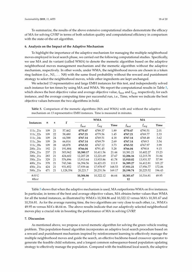
We selected 13 representative and large EMH instances for this test, and independently solvedeach instance for ten times by using MA and WMA. We report the computational results in Table 5,which shows the best objective value and average objective value, fbest and favg, respectively, for eachinstance, and the average computing time per successful run, i.e., Time, where we indicate the bestobjective values between the two algorithms in bold.

Table 5. Comparison of the memetic algorithms (MA and WMA) with and without the adaptivemechanism on 13 representative EMH instances. Time is measured in minutes.

Instances n s ΓWMA MA

fbest favg Time fbest favg Time

111c_21s 109 21 57,462 4770.47 4789.37 1.89 4770.47 4790.51 2.01111c_22s 109 22 58,480 4767.21 4779.56 1.45 4767.21 4769.77 2.33111c_24s 109 24 64,588 4767.14 4769.51 4.18 4767.14 4768.48 3.62111c_26s 109 26 66,814 4767.14 4769.79 2.69 4767.14 4769.5 3.54111c_28s 109 28 68,878 4765.52 4767.12 3.73 4765.52 4767.97 3.99200c_21s 192 21 191,884 8766.04 8791.45 5.28 8766.04 8790.8 9.15250c_21s 237 21 303,962 10,380.17 10,411.56 21.44 10,381.21 10,402.27 15.23300c_21s 283 21 424,602 12,207.28 12,221.69 27.67 12,206.16 12,215.78 31.84350c_21s 329 21 576,896 13,913.64 13,933.86 41.78 13,910.02 13,931.57 57.99400c_21s 378 21 743,346 16,394.56 16,421.03 111.9 16,389.27 16,412.81 101.27450c_21s 424 21 931,852 17,939.46 17,978.97 168.53 17,931.21 17,956.77 172.06500c_21s 471 21 1,128,354 20,221.7 20,231.56 169.17 20,198.74 20,225.52 196.43

#AVG 10,304.86 10,322.12 46.64 10,301.67 10,316.81 49.95#Best 7 12

Table 5 shows that when the adaptive mechanism is used, MA outperforms WMA on five instances.In particular, in terms of the best and average objective values, MA obtains better values than WMAfor all the tested instances, as illustrated by WMA’s 10,304.86 and 10,322.12 versus MA’s 10,301.67 and10,316.81. As for the average running time, the two algorithms are very close to each other, i.e., WMA’s49.95 m versus MA’s 46.64 m. The above results indicate that our adaptively selected neighborhoodmoves play a crucial role in boosting the performance of MA in solving GVRP.

7. Discussion

As mentioned above, we propose a novel memetic algorithm for solving the green vehicle routingproblem. This population-based algorithm incorporates an adaptive local search procedure based ona reward and punishment mechanism inspired by reinforcement learning to effectively manage themultiple neighborhood moves and guide the search, an effective backbone-based crossover operator togenerate the feasible child solutions, and a longest common subsequence-based population updatingstrategy to effectively manage the population. Compared with the traditional local search, the adaptive


local search can manage the different neighborhood moves to adapt to different instances. Comparedto the general crossover operator (such as one-point crossover operator), the backbone-based crossovercan better integrate with the problem structure by inheriting the promising customer and stationsequences from the routes. Based on the extensive experimental results reported earlier, one canobserve that the proposed memetic algorithm is a highly effective heuristic in comparison with thebest-performing methods in the literature for solving the green vehicle routing problem.

8. Conclusions and Future Research

Our proposed memetic algorithm (MA) for the green vehicle routing problem demonstratesthe effectiveness of its key features, including an adaptive local search procedure, a backbone-basedcrossover operator to generate the feasible child solution, and a longest-common-subsequence-basedpopulation updating strategy.

Experimental evaluations on two sets of public benchmark instances show that our MAperforms very favorably compared to the current state-of-the-art reference algorithms in the literature.In particular, MA is able to obtain highly competitive results in terms of both computational efficiencyand solution quality for two sets of the EMH and AB instances. In addition, our computationalstudies demonstrate the effectiveness of the key strategy (i.e., adaptive mechanism to manage multipleneighborhood moves) incorporated into our proposed MA.

The main limitation of this research is the algorithmic generality. The algorithm presented in thispaper does not guarantee the effectiveness of solving other types of GVRP problems, such as GVRPproblems with the popular pickup and delivery constraints. Therefore, in order to solve other variantproblems better, we need to consider adding more general strategies.

These outcomes motivate future research to extend our work in the following directions. First, itwould be interesting to employ a powerful tabu search method (such as granular tabu search [23])to improve the search capability of the adaptive local search phase. Second, the design of ourapproach implies that the development of related procedures that combine its strategies with those ofother population-based frameworks like path-relinking [24] should be very promising. Finally, thesuccess of these ideas for tackling the GVRP problem suggests that it would be worthwhile to testtheir performance in dealing with other variants of the vehicle routing problem [25] or schedulingproblems [26].

Author Contributions: Conceptualization, B.P. and Y.Z.; methodology, B.P. and Y.G.; software, B.P.;writing—original draft preparation, B.P., Y.Z. and Y.G.; writing—review and editing, Y.G. and X.C.; projectadministration, X.C.; funding acquisition, X..

Funding: This research was funded by Fundamental Research Funds for the Central Universities of China(Grant Number: JBK1901011, JBK190504 and JBK1902009), Key Projects of the National Social Science Fund(Grant Number: 16AJL004), Natural Science Foundation of Zhejiang (Grant Number: LQ19G020002), the 13thFive-Year Plan Teaching Reform Project of Higher Education of Zhejiang (Grant Number: jg20180428), the Projectof Education Department of Zhejiang (Grant Number: Y201940902), Basic Scientific Research Project of Wenzhou(Grant Number: R20180002), and Wenzhou Social Sciences Planning Project (Grant Number: 19wsk225).

Conflicts of Interest: The authors declare no conflicts of interest.

References

1. Andelmin, J.; Bartolini, E. A multi-start local search heuristic for the Green Vehicle Routing Problem basedon a multigraph reformulation. Comput. Oper. Res. 2019, 109, 43–63. [CrossRef]

2. Felipe, A.; Ortuño, M.T.; Righini, G.; Tirado, G. A heuristic approach for the green vehicle routing problemwith multiple technologies and partial recharges. Transp. Res. Part E Logist. Transp. Rev. 2014, 71, 111–128.[CrossRef]

3. Dulebenets, M.A. A Delayed Start Parallel Evolutionary Algorithm for just-in-time truck scheduling at across-docking facility. Int. J. Prod. Econ. 2019, 212, 236–258. [CrossRef]

4. Cherkesly, M.; Desaulniers, G.; Laporte, G. A population-based metaheuristic for the pickup and deliveryproblem with time windows and LIFO loading. Comput. Oper. Res. 2015, 62, 23–35. [CrossRef]

http://dx.doi.org/10.1016/j.cor.2019.04.018

http://dx.doi.org/10.1016/j.tre.2014.09.003

http://dx.doi.org/10.1016/j.ijpe.2019.02.017



5. Montoya, A.; Gu´eret, C.; Mendoza, J.E.; Villegas, J.G. A multispace sampling heuristic for the green vehiclerouting problem. Transp. Res. Part C Emerg. Technol. 2016, 70, 113–128. [CrossRef]

6. Erdo˘gan, S.; Miller-Hooks, E. A green vehicle routing problem. Transp. Res. Part E Logist. Transp. Rev.2012, 48, 100–114.

7. Schneider, M.; Stenger, A.; Goeke, D. The Electric Vehicle-Routing Problem with Time Windows andRecharging Stations. Transp. Sci. 2014, 48, 500–520. [CrossRef]

8. Schneider, M.; Stenger, A.; Hof, J. An Adaptive VNS Algorithm for Vehicle Routing Problems withIntermediate Stops. OR Spectrum 2015, 37, 353–387. [CrossRef]

9. Anandakumar, H.; Umamaheswari, K. A bio-inspired swarm intelligence technique for social aware cognitiveradio handovers. Comput. Electr. Eng. 2018, 71, 925–937. [CrossRef]

10. Brezocnik, L.; Fister, I.; Podgorelec, V. Swarm Intelligence Algorithms for Feature Selection: A Review.Appl. Sci. 2018, 8, 1521. [CrossRef]

11. Slowik, A.; Kwasnicka, H. Nature Inspired Methods and Their Industry Applications—Swarm IntelligenceAlgorithms. IEEE Trans. Ind. Inform. 2018, 14, 1004–1015. [CrossRef]

12. Govindan, K.; Jafarian, A.; Nourbakhsh, V. Designing a sustainable supply chain network integratedwith vehicle routing: A comparison of hybrid swarm intelligence metaheuristics. Comput. Oper. Res.2019, 110, 220–235. [CrossRef]

13. Lü, Z.; Hao, J.-K. A memetic algorithm for graph coloring. Eur. J. Oper. Res. 2010, 203, 241–250.14. Fran¸ca, P.M.; Mendes, A.; Moscato, P. A memetic algorithm for the total tardiness single machine scheduling

problem. Eur. J. Oper. Res. 2001, 132, 224–242.15. Benlic, U.; Hao, J.-K. Memetic search for the quadratic assignment problem. Expert Syst. Appl.

2015, 42, 584–595. [CrossRef]16. Cheng, T.C.E.; Peng, B.; Lü, Z. A hybrid evolutionary algorithm to solve the job shop scheduling problem.

Ann. Oper. Res. 2016, 242, 223–237. [CrossRef]17. Pullan, W. A memetic genetic algorithm for the vertex p-center problem. Evol. Comput. 2008, 16, 417–436.

[CrossRef]18. Burke, E.; Cowling, P.; De Causmaecker, P.; Berghe, G.V. A Memetic Approach to the Nurse Rostering

Problem. Appl. Intell. 2001, 15, 199–214. [CrossRef]19. Li, Y.; Lim, A.; Oon, W.-C.; Qin, H.; Tu, D. The tree representation for the pickup and delivery traveling

salesman problem with LIFO loading. Eur. J. Oper. Res. 2011, 212, 482–496. [CrossRef]20. Andelmin, J.; Bartolini, E. An Exact Algorithm for the Green Vehicle Routing Problem. Transp. Sci.

2017, 51, 1288–1303. [CrossRef]21. Birattari, M.; Yuan, Z.; Balaprakash, P.; Stützle, T. F-race and iterated f-race: An overview. In Experimental

Methods for the Analysis of Optimization Algorithms; Springer: Berlin/Heidelberg, Germany, 2010; pp. 311–336.22. Lopez-Ibanez, M.; Dubois-Lacoste, J.; Caceres, L.P.; Birattari, M.; Stützle, T. The IRACE package: Iterated

racing for automatic algorithm configuration. Oper. Res. Perspect. 2016, 3, 43–58. [CrossRef]23. Toth, P.; Vigo, D. The Granular Tabu Search and Its Application to the Vehicle-Routing Problem.

INFORMS J. Comput. 2003, 15, 333–346. [CrossRef]24. Glover, F.; Laguna, M.; Marti, R. Fundamentals of scatter search and path relinking. Control Cybern.

2000, 29, 653–684.25. Franke, T.; Neumann, I.; Bühler, F.; Cocron, P.; Krems, J.F. Experiencing range in an electric vehicle:

Understanding psychological barriers. Appl. Psychol. 2012, 61, 368–391. [CrossRef]26. Hasan, S.M.K.; Sarker, R.; Essam, D.; Cornforth, D. Memetic algorithms for solving job-shop scheduling

problems. Memetic Comput. 2009, 1, 69–83. [CrossRef]

© 2019 by the authors. Licensee MDPI, Basel, Switzerland. This article is an open accessarticle distributed under the terms and conditions of the Creative Commons Attribution(CC BY) license (http://creativecommons.org/licenses/by/4.0/).

http://dx.doi.org/10.1016/j.trc.2015.09.009

http://dx.doi.org/10.1287/trsc.2013.0490

http://dx.doi.org/10.1007/s00291-014-0376-5

http://dx.doi.org/10.1016/j.compeleceng.2017.09.016

http://dx.doi.org/10.3390/app8091521

http://dx.doi.org/10.1109/TII.2017.2786782


http://dx.doi.org/10.1016/j.eswa.2014.08.011

http://dx.doi.org/10.1007/s10479-013-1332-5

http://dx.doi.org/10.1162/evco.2008.16.3.417

http://dx.doi.org/10.1023/A:1011291030731

http://dx.doi.org/10.1016/j.ejor.2011.02.008

http://dx.doi.org/10.1287/trsc.2016.0734

http://dx.doi.org/10.1016/j.orp.2016.09.002

http://dx.doi.org/10.1287/ijoc.15.4.333.24890

http://dx.doi.org/10.1111/j.1464-0597.2011.00474.x

http://dx.doi.org/10.1007/s12293-008-0004-5

http://creativecommons.org/

http://creativecommons.org/licenses/by/4.0/.

Documents

A Memetic Algorithm for the Green Vehicle Routing Problem