Embed Size (px)
Citation preview

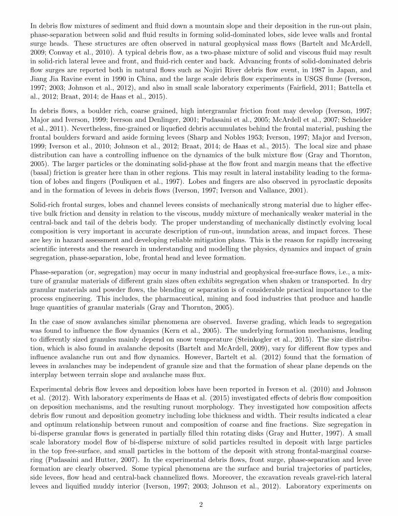
A mechanical model for phase-separation in debris flow
Shiva P. Pudasaini
Department of Geophysics, Steinmann Institute, University of BonnMeckenheimer Allee 176, D-53115, Bonn, Germany
E-mail: [email protected]
Jan-Thomas Fischer
Austrian Research Centre for Forests, Department of Natural HazardsRennweg 1, A-6020, Innsbruck, Austria
Abstract: Understanding the physics of phase-separation between solid and fluid phases as a mixture massmoves down slope is a long-standing challenge. Here, we propose an extension of the two phase mass flow model(Pudasaini, 2012) by including a new mechanism, called separation-flux, that leads to strong phase-separationin avalanche and debris flows while balancing the enhanced solid flux with the reduced fluid flux. The separationflux mechanism is capable of describing the dynamically evolving phase-separation and levee formation in amulti-phase, geometrically three-dimensional debris flow. These are often observed phenomena in naturaldebris flows and industrial processes that involve the transportation of particulate solid-fluid mixture material.The novel separation-flux model includes several dominant physical and mechanical aspects such as pressuregradients, volume fractions of solid and fluid phases and their gradients, shear-rates, flow depth, materialfriction, viscosity, material densities, topographic constraints, grain size, etc. Due to the inherent separationmechanism, as the mass moves down slope, more and more solid particles are transported to the front and thesides, resulting in solid-rich and mechanically strong frontal surge head, and lateral levees followed by a weakertail largely consisting of viscous fluid. The primary frontal solid-rich surge head followed by secondary fluid-rich surges is the consequence of phase-separation. Such typical and dominant phase-separation phenomenaare revealed for two-phase debris flow simulations. Finally, changes in flow composition, that are explicitlyconsidered by the new modelling approach, result in significant changes of impact pressure estimates. Theseare highly important in hazard assessment and mitigation planning and highlight the application potential ofthe new approach.
1 Introduction
Phase-separation and levee formation are often observed phenomena in natural two-phase debris flows, pyro-clastic flows and granular flows in terrestrial and extra terrestrial environments. Examples include lobe depositsfrom 1993 Lascar pyroclastic flows, Chile (Felix and Thomas, 2004), debris flow deposit in Spitsbergen, anddebris flow levees in Sacagawea (Braat, 2014; de Haas et al., 2015). As common phenomena in mountain-ous regions, debris flows fundamentally differ from other types of mass flows, e.g., rock avalanches and dilutesediment-laden water floods. Debris flows contain large amounts of water (typically 20-60% by volume), andthus the mixture composition of solid and fluid governs the rheological properties, and their coupling signifi-cantly influences the flow dynamics (Costa, 1988; Iverson, 1997; Pierson, 2005; Pudasaini, 2012). Debris flowrunout prediction is a major challenge for hazard mitigation in mountain regions, gullies and valleys. Togetherwith the flow volume and basal topography, the inundation area and runout distance may strongly dependon debris flow composition and its evolution (de Haas et al., 2015) and rheology (Pudasaini, 2012). In thepast, several methods have been proposed to predict debris flow dynamics and runout distance including thetopography effects (Pudasaini et al., 2005; Rickenmann, 2005; D’Agostino et al., 2010; Fischer et al., 2012;Mergili et al., 2012), flow volume (Takahashi, 1991; Bathurst et al., 1997; Rickenmann, 1999; Crosta et al.,2004; Berti and Simoni, 2007; Pudasaini and Miller, 2013) or material properties and its composition (Iversonand Denlinger, 2001; Pitman and Le, 2005; Pudasaini et al., 2005; Pirulli, 2009; Scheidl and Rickenmann, 2010;Pudasaini, 2012; Pudasaini and Krautblatter, 2014; Hurlimann et al., 2015; de Haas et al., 2015; Kattel et al.,2016; Kafle et al., 2016).
1
arX
iv:1
610.
0364
9v1
[ph
ysic
s.ge
o-ph
] 1
2 O
ct 2
016
In debris flow mixtures of sediment and fluid down a mountain slope and their deposition in the run-out plain,phase-separation between solid and fluid results in forming solid-dominated lobes, side levee walls and frontalsurge heads. These structures are often observed in natural geophysical mass flows (Bartelt and McArdell,2009; Conway et al., 2010). A typical debris flow, as a two-phase mixture of solid and viscous fluid may resultin solid-rich lateral levee and front, and fluid-rich center and back. Advancing fronts of solid-dominated debrisflow surges are reported both in natural flows such as Nojiri River debris flow event, in 1987 in Japan, andJiang Jia Ravine event in 1990 in China, and the large scale debris flow experiments in USGS flume (Iverson,1997; 2003; Johnson et al., 2012), and also in small scale laboratory experiments (Fairfield, 2011; Battella etal., 2012; Braat, 2014; de Haas et al., 2015).
In debris flows, a boulder rich, coarse grained, high intergranular friction front may develop (Iverson, 1997;Major and Iverson, 1999; Iverson and Denlinger, 2001; Pudasaini et al., 2005; McArdell et al., 2007; Schneideret al., 2011). Nevertheless, fine-grained or liquefied debris accumulates behind the frontal material, pushing thefrontal boulders forward and aside forming levees (Sharp and Nobles 1953; Iverson, 1997; Major and Iverson,1999; Iverson et al., 2010; Johnson et al., 2012; Braat, 2014; de Haas et al., 2015). The local size and phasedistribution can have a controlling influence on the dynamics of the bulk mixture flow (Gray and Thornton,2005). The larger particles or the dominating solid-phase at the flow front and margin means that the effective(basal) friction is greater here than in other regions. This may result in lateral instability leading to the forma-tion of lobes and fingers (Pouliquen et al., 1997). Lobes and fingers are also observed in pyroclastic depositsand in the formation of levees in debris flows (Iverson, 1997; Iverson and Vallance, 2001).
Solid-rich frontal surges, lobes and channel levees consists of mechanically strong material due to higher effec-tive bulk friction and density in relation to the viscous, muddy mixture of mechanically weaker material in thecentral-back and tail of the debris body. The proper understanding of mechanically distinctly evolving localcomposition is very important in accurate description of run-out, inundation areas, and impact forces. Theseare key in hazard assessment and developing reliable mitigation plans. This is the reason for rapidly increasingscientific interests and the research in understanding and modelling the physics, dynamics and impact of grainsegregation, phase-separation, lobe, frontal head and levee formation.
Phase-separation (or, segregation) may occur in many industrial and geophysical free-surface flows, i.e., a mix-ture of granular materials of different grain sizes often exhibits segregation when shaken or transported. In drygranular materials and powder flows, the blending or separation is of considerable practical importance to theprocess engineering. This includes, the pharmaceutical, mining and food industries that produce and handlehuge quantities of granular materials (Gray and Thornton, 2005).
In the case of snow avalanches similar phenomena are observed. Inverse grading, which leads to segregationwas found to influence the flow dynamics (Kern et al., 2005). The underlying formation mechanisms, leadingto differently sized granules mainly depend on snow temperature (Steinkogler et al., 2015). The size distribu-tion, which is also found in avalanche deposits (Bartelt and McArdell, 2009), vary for different flow types andinfluence avalanche run out and flow dynamics. However, Bartelt et al. (2012) found that the formation oflevees in avalanches may be independent of granule size and that the formation of shear plane depends on theinterplay between terrain slope and avalanche mass flux.
Experimental debris flow levees and deposition lobes have been reported in Iverson et al. (2010) and Johnsonet al. (2012). With laboratory experiments de Haas et al. (2015) investigated effects of debris flow compositionon deposition mechanisms, and the resulting runout morphology. They investigated how composition affectsdebris flow runout and deposition geometry including lobe thickness and width. Their results indicated a clearand optimum relationship between runout and composition of coarse and fine fractions. Size segregation inbi-disperse granular flows is generated in partially filled thin rotating disks (Gray and Hutter, 1997). A smallscale laboratory model flow of bi-disperse mixture of solid particles resulted in deposit with large particlesin the top free-surface, and small particles in the bottom of the deposit with strong frontal-marginal coarse-ring (Pudasaini and Hutter, 2007). In the experimental debris flows, front surge, phase-separation and leveeformation are clearly observed. Some typical phenomena are the surface and burial trajectories of particles,side levees, flow head and central-back channelized flows. Moreover, the excavation reveals gravel-rich laterallevees and liquified muddy interior (Iverson, 1997; 2003; Johnson et al., 2012). Laboratory experiments on
2

debris flows have been conducted in rectangular and transversally curved channels to investigate in detail thephase-separation, levee formation, and solid-rich coarse snout (Fairfield, 2011; Battella et al., 2012; Braat, 2014;de Haas et al., 2015). This reveals a strong phase-separation, frontal surge and levee formation. During thedebris motion voids open and close instantaneously. This paves the way for small grains, or fluid, to settle andpercolate in these voids causing vertical sorting which results in solid particles or large boulders accumulationsat the top of the flow (Gray and Thornton, 2005). Tractionless free-surface and friction at the bottom of theflow leads to vertical velocity differences (Braat, 2014). Due to the higher velocity at the upper part of the flowthe free-surface can transport boulder-rich material to the front of the flow. This induces longitudinal sorting.The levees are formed as resistive and coarse-grained debris-flow snouts are shouldered aside by advancingfiner-grained debris (Sharp and Nobles, 1953).
Based on percolation phenomenon, which states that smaller particles preferentially fall into underlying voidspace and uplift large particles towards the free-surface, Gray and Thornton (2005) formulated a model forkinetic sieving (Savage and Lun 1988) of large and small particles in avalanches of dry granular materials.Kinetic sieving is a dominant mechanism in dense granular free-surface flows. Based on this idea there hasbeen recent progress in modeling segregation in bi-disperse granular avalanches (Savage and Lun, 1988; Grayand Thornton, 2005; Shearer et al., 2008; Gray and Ancey, 2009; Gray and Kokelaar, 2010). These models arecapable of predicting the evolution of the size distribution in laboratory experiments (Golick and Daniels, 2009;Wiederseiner et al., 2011). Furthermore, to explain the formation of lateral levees enriched in coarse grains,Johnson et al. (2012) produced data in large-scale debris-flow experiments and combined it with modeling ofparticle-size segregation in a vertical plane. By constructing an empirical velocity field and using it with aparticle-size segregation model (Gray and Thornton, 2005), Johnson et al. (2012) predicted the segregation andtransport of material in the flow in which coarse material segregates to the flow surface, where shear inducesthe transport to the flow front. Moreover, in the flow head, coarse material is overridden, circulated and finallydeposited to form coarse-particle-enriched levees.
Although phase-separation between the solid and fluid phases has a phenomenal and profound effect on debrisflow dynamics, impacts and deposition morphology, no model and simulation exists to describe and dynam-ically simulate the generation and propagation of solid-rich lobes, levees, and surges and the muddy viscousand particle-laden dynamical fluid pool in the central-back and the tail, and in general phase-separation, inthe flow of debris mixture consisting of sediment particles and viscous fluid.
Proper, complete or comprehensive description of these complex flows require a two-phase mixture flow model,including basic flow physics, describing the strong interaction between solid and fluid phases, and at the sametime, an enhanced phase-separation mechanism resulting in solid-rich surges and coarse snout, lateral leveeformation and liquified pool of highly viscous and muddy body and tail. This is the main task of the presentpaper. To do so, here, we enhance the general two-phase mass flow model (Pudasaini, 2012) by introducing init a new separation-flux mechanism to describe the phase-separation phenomena.
2 Phase-separation Mechanism in Mixture Transport
2.1 Two-phase Mass Flow Model
In two-phase debris mixtures, phases are characterized by different material properties. The fluid phase ischaracterized by its material density ρf , viscosity ηf and isotropic stress distribution; whereas the solid phaseis characterized by its material density ρs, internal friction angle φ, the basal friction angle δ, an anisotropicstress distribution, and the lateral earth pressure coefficient K. The subscripts s and f represent the solid andthe fluid phases respectively, with the depth-averaged velocity components for fluid uf = (uf , vf ) and for solidus = (us, vs) in the down-slope (x) and the cross-slope (y) directions. The total flow depth is denoted by h,and the solid-volume fraction by αs (similarly the fluid volume fraction αf = 1 − αs). uf ,us, h and αs are
3

functions of space and time. The solid and fluid mass balance equations are given by (Pudasaini, 2012):
∂
∂t(αsh) +
∂
∂x(αshus) +
∂
∂y(αshvs) = 0,
∂
∂t(αfh) +
∂
∂x(αfhuf ) +
∂
∂y(αfhvf ) = 0.
(1)
Similarly, momentum conservation equations for the solid and the fluid phases, respectively, are:
∂
∂t
[αsh (us − γC (uf − us))
]+
∂
∂x
[αsh
(u2s − γC
(u2f − u2s
)+ βxs
h
2
)]+
∂
∂y
[αsh (usvs − γC (ufvf − usvs))
]= hSxs,
∂
∂t
[αsh (vs − γC (vf − vs))
]+
∂
∂x
[αsh (usvs − γC (ufvf − usvs))
]+
∂
∂y
[αsh
(v2s − γC
(v2f − v2s
)+ βys
h
2
)]= hSys,
∂
∂t
[αfh
(uf +
αs
αfC (uf − us)
)]+
∂
∂x
[αfh
(u2f +
αs
αfC(u2f − u2s
)+ βxf
h
2
)]+
∂
∂y
[αfh
(ufvf +
αs
αfC (ufvf − usvs)
)]= hSxf
,
∂
∂t
[αfh
(vf +
αs
αfC (vf − vs)
)]+
∂
∂x
[αfh
(ufvf +
αs
αfC (ufvf − usvs)
)]+
∂
∂y
[αfh
(v2f +
αs
αfC(v2f − v2s
)+ βyf
h
2
)]= hSyf .
(2)
In (2), the source terms are as follows:
Sxs = αs
[gx − us
|us|tan δpbs − εpbs
∂b
∂x
]− εαsγpbf
[∂h
∂x+∂b
∂x
]+ CDG (uf − us) |uf − us|−1, (3)
Sys = αs
[gy − vs
|us|tan δpbs − εpbs
∂b
∂y
]− εαsγpbf
[∂h
∂y+∂b
∂y
]+ CDG (vf − vs) |uf − us|−1, (4)
Sxf= αf
[gx − ε
[1
2pbf
h
αf
∂αs
∂x+ pbf
∂b
∂x− 1
αfNR
{2∂2uf∂x2
+∂2vf∂y∂x
+∂2uf∂y2
− χufε2h2
}
+1
αfNRA
{2∂
∂x
(∂αs
∂x(uf − us)
)+
∂
∂y
(∂αs
∂x(vf − vs) +
∂αs
∂y(uf − us)
)}− ξαs (uf − us)
ε2αfNRAh2
]]
−1
γCDG (uf − us) |uf − us|−1,
(5)
Syf = αf
[gy − ε
[1
2pbf
h
αf
∂αs
∂y+ pbf
∂b
∂y− 1
αfNR
{2∂2vf∂y2
+∂2uf∂x∂y
+∂2vf∂x2
− χvfε2h2
}
+1
αfNRA
{2∂
∂y
(∂αs
∂y(vf − vs)
)+
∂
∂x
(∂αs
∂y(uf − us) +
∂αs
∂x(vf − vs)
)}− ξαs (vf − vs)
ε2αfNRAh2
]]
−1
γCDG (vf − vs) |uf − us|−1.
(6)
The pressures and the other parameters involved in the above model equations are as follows:
βxs = εKxpbs , βys = εKypbs , βxf= βyf = εpbf , pbf = −gz, pbs = (1− γ)pbf ,
CDG =αsαf (1− γ)
[εUT {PF(Rep) + (1− P)G(Rep)}], F =
γ
180
(αf
αs
)3
Rep, G = αM(Rep)−1f ,
γ =ρfρs, Rep =
ρfd UTηf
, NR =
√gLHρfαfηf
, NRA =
√gLHρfAηf
, αf = 1− αs, A = A(αf ).
(7)
Equations (1) are the depth-averaged mass balances for solid and fluid phases respectively, and (2) are thedepth-averaged momentum balances for solid (first two equations) and fluid (other two equations) in the x-and y-directions, respectively.
4
In the above non-dimensional equations, x, y and z are coordinates in down-slope, cross-slope and flow normaldirections, and gx, gy, gz are the respective components of gravitational acceleration. L and H are the typicallength and depth of the flow, ε = H/L is the aspect ratio, and µ = tan δ is the basal friction coefficient. CDG
is the generalized drag coefficient. Simple linear (laminar-type, at low velocity) or quadratic (turbulent-type,at high velocity) drag is associated with = 1 or 2, respectively. UT is the terminal velocity of a particleand P ∈ [0, 1] is a parameter which combines the solid-like (G) and fluid-like (F) drag contributions to flowresistance. pbf and pbs are the effective fluid and solid pressures. γ is the density ratio, C is the virtual masscoefficient (kinetic energy of the fluid phase induced by solid particles), M is a function of the particle Reynoldsnumber (Rep), χ includes vertical shearing of fluid velocity, and ξ takes into account different distributions ofαs. A is the mobility of the fluid at the interface, and NR and NRA respectively, are the quasi-Reynoldsnumber and mobility-Reynolds number associated with the classical Newtonian and enhanced non-Newtonianfluid viscous stresses. Slope topography is represented by b = b(x, y).
2.2 A Novel Mechanical Model for Phase-separation in Mixture Flows
Without any complex mechanical knowledge of the phase-separation mechanism, it can phenomenologicallybe summarized as follows: Mass fluxes are described for each material phase in the mass balances (1), whereno explicit phase interaction and separation terms appear. Without any additional separation-fluxes the solidand fluid materials would tend to homogeneously move down-slope, preventing significant to strong phase-separation, which is often observed in field events and laboratory experiments (Iverson, 1997; 2003; Fairfield,2011; Battella et al., 2012; Johnson et al., 2012; Braat, 2014; de Haas et al., 2015). An increase, e.g., of solidmaterial flux results in more solid material farther downslope, while in the mean time, a respectively reducedseparation-flux for the fluid material results in more fluid material farther upslope. The same process canbe applied to the lateral direction: solid material fluxes are enhanced outward from the longitudinal centralline, and conversely, the fluid material fluxes are enhanced inward to the longitudinal central line. This bringsmore solid material towards the outer and frontal regions and more fluid material towards the center and backof the flow. Longitudinal or lateral phase separation fluxes can be considered separately as uni-directionalphase-separations. More complex and complete situations require combining both the longitudinal and lateralseparation-fluxes and the resulting phase-separations, as often observed in field events or laboratory debris flowexperiments (de Haas et al., 2015).
While mass flux induced phase separation appears to be phenomenologically clear, here, we develop a newmechanical model to describe the phase-separation in two-phase debris flows. This mechanical approach ap-propriately accounts for phase-separation processes in geometrically three-dimensional mixture mass flows.
2.2.1 The Relative Velocity
For the purpose of developing separation flux models, we formulate the total net force balance taking intoaccount the forces, that appear in the source terms in (3) and the pressure gradients, that appear in the fluxterm of the solid momentum balance in (2). Additionally, the solid shear forces may be considered in thetotal net force balance. For simplicity, we consider only the linear drag, i.e., = 1. Ignoring the inertialand acceleration terms, the relative velocity between solid and fluid, u∗r = uf − us, is expressed dividing thenet force balance by the drag coefficient CDG. The relative velocity u∗r is of key importance for the phase-separation mechanism, which is directly linked to the net forces that appear in the system. The down-slope solidmomentum equation indicates that the relative velocity u∗r results from different effective force contributions,including:
u∗r = f (FC , FP , FB, FT , FS , . . .) = 1CDG
(FC + FP + FB + FT + FS + . . .) , (8)
where FC is the Coulomb force, FP is the force due to the lateral hydraulic pressure gradient, FB is the forceassociated with buoyancy, FT emerges from the topographic pressure gradient, and FS is related to the shear
5
force. For convenience, written in dimensional form, these force components are:
FC = µ(1− γ)αsρsg cos ζ, FP =Kx
2(1− γ)ρsg cos ζ
(h∂αs
∂x
)+Kx(1− γ)ρsg cos ζ
(αs∂h
∂x
),
FB = γρsg cos ζ
(αs∂h
∂x
), FT = ρsg cos ζ
(αs∂b
∂x
), FS = χs αsµs
ush2s.
(9)
Similar to the hydraulic pressure gradient, the topographic pressure gradient also may contribute to phase-separation. Another force which also contributes to the phase-separation is the velocity shearing (shear-rate)in the xy-, xz- and yz-planes. Although shearing is virtually neglected in the depth-averaged models, itmay contribute to phase-separation and can be revived. Furthermore, depending on the flow situation, thisshearing may be localized in a thin layer, or otherwise may be present through the entire flow depth (Domnikand Pudasaini, 2012; Domnik et al., 2013). This has been included in the above expression through theapproximated shear-rate γxz ≈ us/h
2s (any other suitable expression can be used), where χs is the shear
factor, and µs is the dynamic viscosity (Pudasaini, 2012), resulting the shear-force FS in (9). Moreover, thecorresponding expression for the relative velocity v∗r in the lateral y-direction can be constructed. However,any other physically important and relevant forces can be included in (8), and thus in the list (9). Examplesmay include cohesion, and electrostatic forces.
2.2.2 Separation Fluxes
Here, we develop a new mechanical model for separation fluxes resulting in separation between solid and fluidin a mixture flow. Let k represents one of the n phases in the mixture and m represents the subscript associatedwith the (bulk) mixture. The mixture density ρm, the mass fraction Ck of the phase k, the mixture velocityum, and the mixture mass flux ρmum are given by (Manninen et al., 1996; Krasnopolsky et al., 2016)
ρm =∑αkρk, Ck =
αkρkρm
, um =1
ρm
∑αkρkuk =
∑Ckuk, ρmum =
∑αkρkuk, (10)
where∑αk = 1 is the holdup constraint, and um = (um, vm, wm) are the mixture velocity components along
the downslope x, cross-slope y and flow depth direction z, respectively. For any phase k, the full dimensionalphase mass balance equation is given by:
∂
∂t(αkρk) +
∂
∂x(αkρkuk) +
∂
∂y(αkρkvk) +
∂
∂z(αkρkwk) = 0. (11)
The slip velocity ufk of the phase k with respect to the velocity of a background (continuum) phase f , and thediffusion velocity uDk
of the phase k, respectively, are denoted by
ufk = uk − uf ; uDk= uk − um. (12)
Then, the diffusion velocity uDl= ul−um of a dispersive phase l can be represented by (Manninen et al., 1996)
uDl= ufl −
∑Ckufk . (13)
Here, we are mainly concerned with the two-phase solid-fluid mixture flow. For the mixture consisting of afluid-phase f and a single dispersive (particle, or) solid-phase s (13) reduces to
uDs = ufs − Csufs = (1− Cs)ufs = (Cs − 1) u∗r , (14)
where, Cs = αsρs/ρm, and u∗r = −ufs is the relative (or, slip) velocity between the solid and the fluid phasesthat can be obtained from the momentum balance, as shown in Section 2.2.1. Here, u∗r indicates the fullnon-depth-averaged velocity field such that u∗r is its mean (depth-averaged) value. u∗r should contain all theforces resulting in slip velocity that yields phase separation. For the ease of notation, here, we drop tildefrom the corresponding variables until we again introduce the depth-averaged variables while developing thedepth-averaged enhanced mass balance equations. The expressions as in (8) and (9) can also be derived forthe full non-depth averaged descriptions of the relative velocities (u∗r , v
∗r , w
∗r) in all three flow directions.
6

The diffusion velocity for the fluid-phase, uDf, can be written as:
uDf= uf − um = uf − (us − uDs) = u∗r + uDs = u∗r + (Cs − 1)u∗r = Csu∗r . (15)
Expressions similar to (14 ) and (15) can be analogously derived for the y- and z- directions:
vDs = (Cs − 1) v∗r , vDf= Csv∗r ; wDs = (Cs − 1)w∗
r , wDf= Csw∗
r . (16)
For a mixture consisting of a solid and a fluid phase (11) reduces, respectively, to the solid and fluid phasemass balance equations as:
∂
∂t(αsρs) +
∂
∂x(αsρsus) +
∂
∂y(αsρsvs) +
∂
∂z(αsρsws) = 0, (17)
∂
∂t(αfρf ) +
∂
∂x(αfρfuf ) +
∂
∂y(αfρfvf ) +
∂
∂z(αfρfwf ) = 0. (18)
Summing up (17) and (18) and using (10) yields the (bulk) mixture mass balance:
∂
∂t(ρm) +
∂
∂x(ρmum) +
∂
∂y(ρmvm) +
∂
∂z(ρmwm) = 0, (19)
which can be written as[∂
∂t(αsρs) +
∂
∂x(αsρsum) +
∂
∂y(αsρsvm) +
∂
∂z(αsρswm)
]+
[∂
∂t(αfρf ) +
∂
∂x(αfρfum) +
∂
∂y(αfρfvm) +
∂
∂z(αfρfwm)
]= 0.
(20)
From (12) with the diffusion velocities, (20) reduces to[∂
∂t(αsρs) +
∂
∂x
(αsρs
{us − uDs
})+
∂
∂y
(αsρs
{vs − vDs
})+
∂
∂z
(αsρs
{ws − wDs
})]+
[∂
∂t(αfρf ) +
∂
∂x
(αfρf
{uf−uDf
})+
∂
∂y
(αfρf
{vf−vDf
})+
∂
∂z
(αfρf
{wf−wDf
})]= 0.
(21)
Inserting the expressions for uDs , uDf; vDs , vDf
; wDs , wDffrom (14), (15) and (16 ), this becomes:[
∂
∂t(αsρs)+
∂
∂x
(αsρs
{us+
αfρfρm
u∗r
})+∂
∂y
(αsρs
{vs+
αfρfρm
v∗r
})+∂
∂z
(αsρs
{ws+
αfρfρm
w∗r
})]+
[∂
∂t(αfρf )+
∂
∂x
(αfρf
{uf−
αsρsρm
u∗r
})+∂
∂y
(αfρf
{vf−
αsρsρm
v∗r
})+∂
∂z
(αfρf
{wf−
αsρsρm
w∗r
})]=0.
(22)
This can be split into dynamically coupled and balanced system of mass conservations for solid and fluid phases:
∂
∂t(αsρs)+
∂
∂x
(αsρs
{us +
αfρfρm
u∗r
})+∂
∂y
(αsρs
{vs +
αfρfρm
v∗r
})+∂
∂z
(αsρs
{ws +
αfρfρm
w∗r
})=0, (23)
∂
∂t(αfρf )+
∂
∂x
(αfρf
{uf −
αsρsρm
u∗r
})+∂
∂y
(αfρf
{vf −
αsρsρm
v∗r
})+∂
∂z
(αfρf
{wf −
αsρsρm
w∗r
})=0. (24)
This splitting is legitimate and appears naturally when viewed (interpreted) in terms of a coupled system,preserving the total mass balance, because adding (23) and (24) results in the entire system (19). The advantageof the dynamically coupled system is that without adding or losing any mass the system (23) and (24) enhancesthe solid mass flux by the amount + (αsαfρsρf/ρm)u∗r , and the fluid mass flux is reduced by the same amount− (αsαfρsρf/ρm)u∗r in the downslope x-direction. The same holds in other flow directions, y and z, thetransversal and flow depth directions. These enhanced and reduced fluxes for the solid and fluid are separatingthe solid and fluid mass flows resulting in the phase-separation in the mixture. Furthermore, the new separationflux models (23) and (24) are free of any empirical parameters and are derived without any assumptions.
7

Since the material phase densities ρs and ρf are constant, (23) and (24) can be further simplified:
∂αs
∂t+
∂
∂x
(αsus +
γ αsαf
αs + γαfu∗r
)+
∂
∂y
(αsvs +
γ αsαf
αs + γαfv∗r
)+
∂
∂z
(αsws +
γ αsαf
αs + γαfw∗r
)= 0, (25)
∂αf
∂t+
∂
∂x
(αfuf −
αsαf
αs + γαfu∗r
)+
∂
∂y
(αfvf −
αsαf
αs + γαfv∗r
)+
∂
∂z
(αfwf −
αsαf
αs + γαfw∗r
)= 0. (26)
In the derivation of the depth-averaged models, it is legitimate to assume that the velocity scaling in the flowdepth direction can be some orders of magnitude smaller than the velocity scaling in the longitudinal andlateral flow directions (Savage and Hutter, 1989). Then, following the standard procedures (Pitman and Le,2005; Pudasaini, 2012) the mass balance equations (25) and (26) can be depth averaged to yield:
∂
∂t(αsh) +
∂
∂x
(αshus +
γ hαsαf
αs + γαfu∗r
)+
∂
∂y
(αshvs +
γ hαsαf
αs + γαfv∗r
)= 0, (27)
∂
∂t(αfh)+
∂
∂x
(αfhuf −
hαsαf
αs + γαfu∗r
)+∂
∂y
(αfhvf −
hαsαf
αs + γαfv∗r
)= 0, (28)
where all the dynamical variables involved are now the depth-averaged quantities.
For convenience, we introduce the notations for separation fluxes for solid(SFxs, SF
ys
)and fluid
(SFxf, SF
yf
)in
the down-slope and cross-slope directions, respectively,
SFxs
= λpsu∗rαsαfh, S
Fxf
= λpfu∗rαsαfh; SF
ys = λpsv∗rαsαfh, S
Fyf
= λpfv∗rαsαfh, (29)
where λps = γ/ (αs + γαf ) and λpf = 1/ (αs + γαf ). The structure in (29) indicates, that the separation fluxes(SFxs,f
;SFys,f
)vanish for vanishing αs, αf and h.
2.2.3 Phase Separation Model Equations
With the separation fluxes (29), the model equations for the enhanced solid and fluid mass balances (27) and(28) yield (Pudasaini, 2015):
∂
∂t(αsh) +
∂
∂x
(αshus + SF
xs
)+
∂
∂y
(αshvs + SF
ys
)= 0, (30)
∂
∂t(αfh)+
∂
∂x
(αfhuf − SF
xf
)+∂
∂y
(αfhvf − SF
yf
)=0. (31)
Equations (30) and (31), together with momentum balances (2), constitute a set of novel mechanical modelequations (Pudasaini, 2015) capable of describing a three-dimensional time and spatial evolution of complexphase-separation phenomena in two-phase debris, or mass flows. Importantly, by appropriately switching thesigns of the separation fluxes, the phase-separations can be reversed. Such a switch can also be applied to gainmixing in two-phase flows and inherently depends on the material (phase) interaction processes and properties.
It is important to mention that due to the strong phase interactions, considering only the momentum equationsand the applied forces therein would not yield realistic phase-separation magnitudes. This is a very importantand novel finding for phase-separation in mixture flows. So, in order to model the phase-separation in two-phase
debris mixture flows, the separation-fluxes(SFxs, SF
xf
)and
(SFys , S
Fyf
), as emerged in the derivations (30) and
(31), must be considered in the down-slope and cross-slope solid and fluid fluxes, in the solid and fluid massbalances, respectively. As mentioned earlier, this does not affect the mass balances for solid and fluid because,this process does not induce additional mass production or loss.
There are several mechanically important aspects in the separation fluxes in (30) and (31). These appear mainlyin the solid and fluid separation fluxes (29). Flux separations are triggered by inter-phase forces, resulting in thenon-zero slip velocities u∗r and v∗r . These separation fluxes are amplified simultaneously by the solid and fluid
8

volume fractions through their product αsαf . The magnitude is further amplified or controlled by the total(mixture) flow height and the density ratio. Furthermore, the separation flux magnitude is uniformly reduced
by the factor 1/ (αs + γαf ) for all the separation flux components(SFxs, SF
ys
)and
(SFxf, SF
yf
). Moreover, the
separation fluxes can be triggered in one or more flow directions, and depending on the flow dynamics thesecan be different as indicated by u∗r and v∗r , which, in general, can be different quantities. The most importantcharacteristic of the separation fluxes is that separation ceases as soon as one of the components (eitherαs, or αf ) in the mixture vanishes. This is a natural condition, because if the presence of the counter (or,complementary) component vanishes nothing needs to be separated.
2.2.4 Model Reduction
The relative (or, slip) velocities (u∗r , v∗r ), that trigger the phase separation mechanisms, have been presented
in Section 2.2.1. In simple situations, it may suffice to consider only some particular force components for u∗r(and v∗r ) in (9). To begin with, we consider the pressure gradient FP . For the sake of simplicity, and withoutloss of generality, we may assume that the gradient of the total debris is dominated by the gradient of the solidvolume fraction, and that ∂αs/∂x and ∂αs/∂y can be approximated or parameterized (say, αspx as a functionof x, or simply a parameter; similarly αspy ). Alternatively, we could also assume that λps (∂αs/∂x) ≈ const.and λps (∂αs/∂y) ≈ const. Then, the separation fluxes are:
SFxs
= SRxsαsαfh, S
Fys = SR
ysαsαfh; SFxf
= SRxfαsαfh, S
Fyf
= SRyfαsαfh, (32)
where, the separation-rates SRxs,f
and SRys,f
are given by:
SRxs
=1
2
Kx
CDG(1− γ)ρsg cos ζλps
(h∂αs
∂x
), SR
ys =1
2
Ky
CDG(1− γ)ρsg cos ζλps
(h∂αs
∂y
);
SRxf
=1
2
Kx
CDG(1− γ)ρsg cos ζλpf
(h∂αs
∂x
), SR
yf=
1
2
Ky
CDG(1− γ)ρsg cos ζλpf
(h∂αs
∂y
).
(33)
The advantage of utilizing the terminology separation-flux is that it can be considered as a general function ofthe separation-rate, solid and fluid volume fractions and the flow depth. Consequently, the separation velocityemerges from separation-flux as a function of the relative phase velocity, volume fractions of solid or fluid, andthe factor λps,f . The relations (32) indicate that structurally SR
xsαf = λpsu
∗rαf =: use and SR
xfαs = λpfu
∗rαs =: ufe
are the effective down-slope separation velocities for solid and fluid phases, respectively. Thus, λps,f are theseparation-rate, or the separation-velocity intensity factors. The effective cross-slope separation velocities forsolid and fluid phases can be obtained analogously. This indicates that the effective separation velocity for solidvaries with the local volume fraction of fluid and the separation-rate for solid. Some important aspects of (33) inits form are as follows: As the true solid density approaches the true fluid density, the buoyancy reduced normalload of the solid vanishes. Consequently, solid and fluid are close to neutrally buoyant condition so that bothphases tend to move together (Pudasaini, 2012). This reduces the phase-separation intensity. Furthermore, asthe drag increases, the two phases come closer, resulting in the reduction of the phase-separation.
In general, depending on the complexity of the flow configuration and phase-separation, all force componentsFi that influence the relative velocities u∗r and v∗r can contribute to the separation fluxes. Then, the separation-rates (33) can be written in general form as:
SRxs
= λpsu∗r , S
Rys = λpsv
∗r ; SR
xf= λpfu
∗r , S
Ryf
= λpfv∗r . (34)
Furthermore, in the new separation flux approach, terrain slope changes the apparent forces, and changes ofmass flux are represented by separation fluxes. Such observations for snow avalanches (Bartelt et al., 2012) arein line with new model approach.
Concentration gradients, that are key parameters in the separation mechanism (33), may require proper treat-ments after an optimum or desired separation has been achieved. This may demand for some upper and/or thelower limits of the solid concentration gradients, which could be important for technical and applied problems.As in chemical phase-separation process (Hillert, 1956; Cahn and Hilliard, 1958; Vladimirova et al., 1999), this
9

may result in near phase-equilibrium. The systematic emergence of SRxs,f
and SRys,f
in (30) and (31) result in acomplex non-linear anti-diffusion (see, Section 2.2.5) of solid volume fraction that acts in combination with theother non-linear expressions in fluid momentum equations in (2) and (5)-(6) that resulted from non-Newtonianviscous stress emerging from the solid fraction distribution (the terms associated with NRA
). This connectionbetween the solid volume fraction gradients balances the dynamics of the concentration gradients in (33).
The new separation flux model can also be compared to the results of the pioneering work by Gray and Thorn-ton (2005), where segregation originates from pressure gradients. In their formulation, simple drag or the Darcylaw was used with bulk velocity in a dry granular mixture consisting of particles of different sizes. Down-slopeand cross-slope separations were ignored. Bulk velocity is prescribed, and the transport equation for volumefraction was used without the mixture momentum equations. The segregation-rate for a mixture of small andbig solid particles as derived by Gray and Thornton (2005) (also see, Johnson et al., 2012) can be realizedfrom (33) with SR
x = (B/c)g cos ζ, where B is a perturbation constant and c is a simple drag coefficient. So,Gray and Thornton (2005), which includes an ad-hoc constraint on the pressure scaling, can be related to thepressure gradients FP .
Here, we have fundamentally advanced in modelling and simulating two-phase, and geometrically three-dimensional phase-separations in a real two-phase debris flow consisting of a mixture of essentially two dif-ferent materials, solid particles and viscous fluid. In contrast to Gray and Thornton (2005), in our model,(SRxf6= SR
xs;SR
yf6= SR
ys
)are possible, resulting from different material properties for the solid and fluid con-
stituents. Our new model includes phase-separation in both flow directions. The new mechanical modelincludes several contributing factors leading to phase-separation. As the model is fully coupled with solid andfluid phase mass and momentum balances no assumption on the bulk and slip velocities is required. The newmethod now presents a possibility to simulate time and spatial evolution of phase-separation in mixture flows.
2.2.5 Up-hill Diffusion and Separation-potential
Here, we show that the enhanced solid mass balance (30) describes the phase-separation as an advection, andup-hill diffusion process. Similar analysis also holds for fluid. Up-hill diffusion is a typical process in thedirection against the concentration gradient resulting in phase separation in mixture (e.g., alloy) (Hillert, 1956;Cahn and Hilliard, 1958). This anti-diffusion process essentially leads to phase-separation in the flow of adebris mixture. For simplicity, in this Section, we only consider the flow along down-slope. Without loss ofgenerality, we assume that the variation of h with x is negligible. Then, from (30) and (33), we obtain
∂αs
∂t+
∂
∂x(αsus) +
∂
∂x
(Da
s
∂αs
∂x
)= 0, (35)
where, the coefficient of anti-diffusion, Das , is Da
s = (Kx/2CDG) (1− γ)ρsg cos ζλpsαsαfh. Since Das > 0, (35)
governs an advection, and an anti-diffusion for αs, which advects with us and diffuses up-hill with Das . Fur-
thermore, in analogy to the chemical-potential in alloy (Hillert, 1956; Cahn and Hilliard, 1958; Vladimirova etal., 1999), αs in the diffusion term in (35) is called the separation-potential. However, unlike in the chemical-potential, here, the anti-diffusion coefficient Da
s is a complex function of several physical and mechanicalquantities, and the flow variables, including the solid and fluid volume fractions, and the flow height. Itclearly shows that the phase separation is triggered by the concentration gradient ∂αs/∂x, or effectively thenon-zero separation-potential, and it is amplified (or, reduced) by the magnitude of Da
s . Furthermore, thephase-separation ceases either, when the gradient ∂αs/∂x is close to zero, or when the flow is neutrally buoy-ant, or if locally one of the phases is negligible. Phase-separation varies inversely with the drag coefficient,which means the phase-separation process is faster in a mixture with less viscous fluid than the same in themixture with more viscous fluid.
3 Simulation Set-up, Parameters, and Numerical Method
To assess the capabilities of the new separation-flux model, two-phase flow simulations are performed down aninclined slope with angle ζ = 45◦. Initially, the uniform mixture consists of 50% solid particles and 50% viscousfluid, kept in a triangular-wedge x ∈ (0, 50) m, y ∈ (−35, 35) m that is released instantaneously. The model and
10
material parameter values chosen for the simulation are: φ = 35◦, δ = 15◦, ρf = 1, 100 kg m−3, ρs = 2, 500 kgm−3, NR = 30, 000, NRA = 1, 000, Rep = 1, UT = 1.0 ms−1, P = 0.5, = 1, χ = 0, ξ = 0, C = 0.0. Theseparameter selections are based on the physics of two-phase mass flows (Pudasaini, 2012, 2014; Pudasaini andKrautblatter, 2014; Kafle et al., 2016; and Kattel et al., 2016). To highlight the process, the separation-rates(SR
s , SRf ) can be estimated as follows: for dilatational flows, with the above values of φ and δ, K is about 0.3
(Pudasaini and Hutter, 2007), for a relatively dense flow CGD is of order unity (Pudasaini, 2012). Consideringa typical flow height of about 2 m and a gentle deviation of ∂αs/∂x from a local equilibrium (e.g., 0.005 m−1),for a typical solid fraction of 0.65, the separation-rate intensity factors are obtained as (λps, λ
pf ) ≈ (0.55, 1.20).
Then, the separation rates as estimated from (33) are (SRs , S
Rf ) ≈ (5, 10) ms−1. The separation rate SR
s = 5
ms−1 is a reasonable estimate for the enhancement of the solid separation flux on inclined surface. With this,the separation velocity for solid is about 1.75 ms−1. This indicates that phase separation is a fairly fast process.Although it depends on the flow configuration and dynamics, it is a reasonable velocity enhancement for thesolid as the flow velocity can be on the order of 10 ms−1. Similar analysis holds for the fluid phase. Since,for the flow considered here, (SR
s , SRf ) = (5, 10) ms−1 produce similar results as (33), we chose these values for
simulation. Otherwise, in real and more complex debris flows SRs , and SR
f should be computed from (33) or(34).
The model equations (30) and (31), together with momentum balances (2) are a set of well-structured, non-linear hyperbolic-parabolic partial differential equations in conservative form with complex source terms (Pu-dasaini, 2012; Kafle et al., 2016). These model equations are used to compute the total debris depth h, solidvolume fraction αs, velocity components for solid (us, vs), and for fluid (uf , vf ) in x- and y-directions, re-spectively, as functions of space and time. The model equations are solved in conservative variables W =(hs, hf ,mxs ,mys ,mxf
,myf )t, where hs = αsh, hf = αfh are the solid and fluid contributions to the debris mix-ture, or the flow height; and (mxs ,mys) = (αshus, αshvs), (mxf
,myf ) = (αfhuf , αfhvf ), are the solid and fluidmomenta. This facilitates numerical integration even when shocks are formed in the field variables (Pudasaini,2014; Kattel et al., 2016). The high-resolution shock-capturing Total Variation Diminishing Non-OscillatoryCentral (TVD-NOC) scheme has been implemented (Tai et al., 2002; Pudasaini and Hutter, 2007; Domniket al., 2013; Pudasaini and Krautblatter, 2014). Advantages of the applied innovative and unified simulationtechnique for real two-phase debris flows and the corresponding computational strategy have been explainedin Kafle et al. (2016) and Kattel et al. (2016).
4 Simulating Phase-separation in Mixture Flows
Next, we simulate phase separation between solid and fluid phases as a two-phase debris mass moves downslope. By applying the two-phase debris flow model (Pudasaini, 2012), enhanced with the new separation-fluxmechanism the predominant phenomena are revealed in Fig. 1 and Fig. 2 for debris flow simulations.
4.1 Time Evolution of Bi-directional Phase-separation
Multi-directional phase separations are observed in many mixture flows. Examples include the debris flowexperiments by Johnson et al. (2012) and de Haas et al. (2015). In this section the simulation and analysisof the phase separation in complex flow situation that simultaneously includes phase separations both in thelongitudinal and lateral directions is described. The analysis has been presented with the detailed investigationsbased on the dynamics of the solid-phase, fluid-phase and the total debris mixture. Most importantly, a frontalsurge and largely solid-rich mechanically very strong frontal wall and lateral levee walls, followed by relativelyweak viscous fluid in the flow body and tail are observed.
4.1.1 Bi-directional Solid Phase-separation
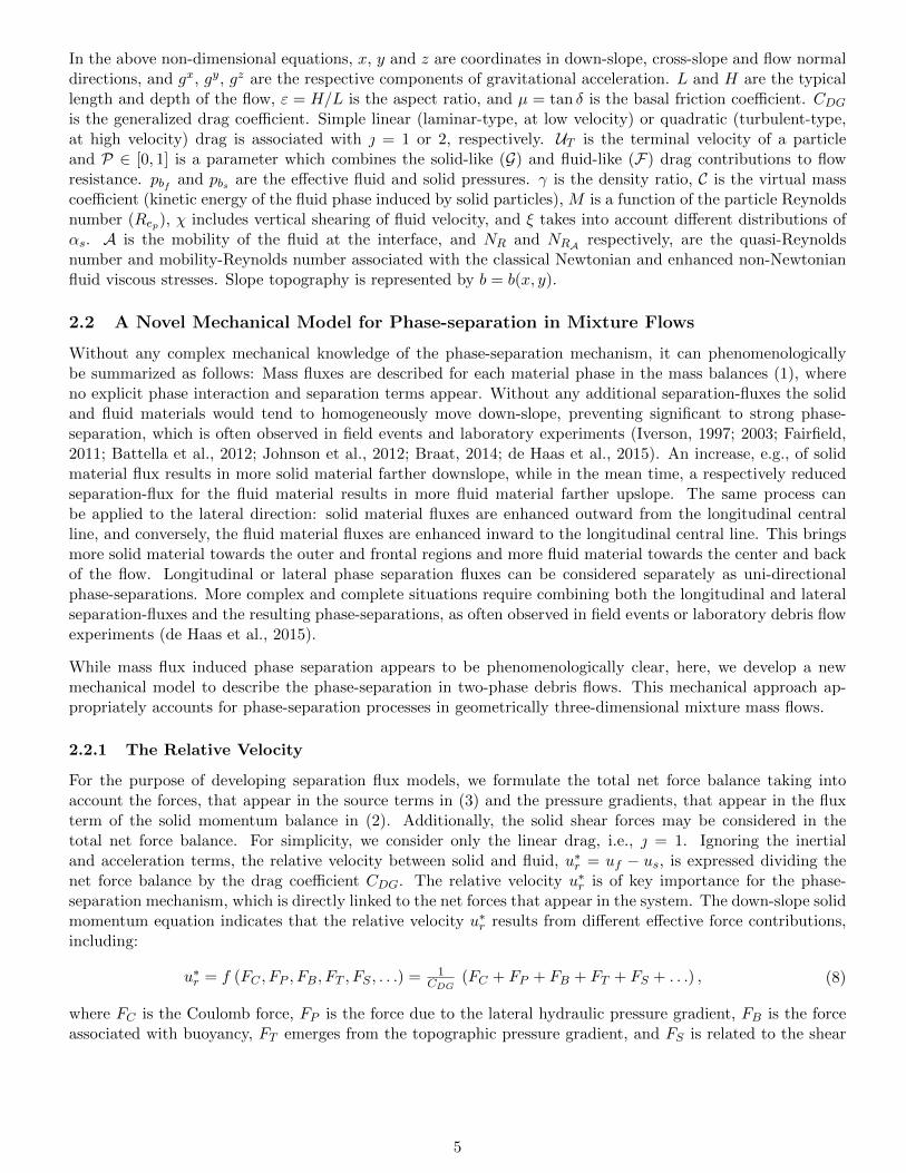
Bi-directional phase-separation is presented in Fig. 1. The figure displays the time evolution of the phaseseparation for t = 0, 1, 2, 3, 4, 4.5 s. The left panels A show the bi-directional solid phase-separation. Thisincludes the separation of solid from the fluid in both the down-slope and cross slope directions. To obtainsuch phase-separation, the simulation considers the enhanced solid separation-fluxes in both the flow directions.Similarly, the reduced fluid separation-fluxes are applied in both the flow directions. As soon as the debris
11

mass is released the solid-phase separation takes place already at t = 1 s. This process separates solid from thefluid from initially uniformly mixed debris material and pushes the solid material to the sides and to the frontof the dominantly downward moving debris body. Although phase separations are effective in both directions,immediately after the flow release, the solid separation appears to be dominating in the lateral direction untilt = 1 s, afterwards, separation also becomes stronger in the down-slope direction. Lateral solid walls beginto develop around t = 1 s. Then, these levees are pushed outward and apart in the cross-slope. This processintensifies for t > 1 s. As the down-slope solid separation gains pace for t ≥ 2 s, the solid levees are connected inthe front of the moving mass, thus forming frontal surge of solid material. The intensity of the lateral separationof solid also depends, including other forces, on the competition between the gravity forces, pressure gradients,and the phase separation-fluxes. As time elapses, from t = 2 s to t = 4.5 s the separation intensifies. In time, thephase-separation induced strong solid lateral levees and a frontal surge-head are amplified. As the solid massmigrates rapidly to the lateral sides and to the front of the flow, due to the mass balance, the amount of solid inthe back and the center of flow is largely reduced. This forms a beautiful three-dimensional double-wing shockwave of solid fraction. This coupled hydrodynamic shock-wave is sharpened and consolidated in the front head,and progressively widens and thins in the rear-lateral portion of the solid mass. The emergence, evolution andpropagation of such a fish-tail-like solid structure is novel in simulating two-phase solid-fluid mixture flow.
4.1.2 Bi-directional Fluid Phase-separation
The middle panels B in Fig. 1 display the process of fluid phase-separation which is the reverse of the solidphase-separation. Separation-fluxes for fluid bring more and more fluid to the back and central regions of thedebris mass. In fact, the solid mass is transported to the lateral sides and front of the debris body. This is howthese processes and solid and fluid mass evolutions (migrations) are reversed to each other. As the debris massis released, at first slowly then rapidly, the fluid mass is accumulating in the center and back of the debris bodyas indicated by the amount of the fluid in panels B. The phase-vacuum, induced by the solid phase-separation,has been filled by the now separated fluid, thus, creating the viscous and particle-laden fluid (pool) in thecenter-and-back of the debris body. The solid concentration minimizes along the central line and decreases tothe tail side while the fluid concentration is enhanced in this region. With respect to the amount of fluid, thispool is shallow in the front, side, and rear, i.e., along the frontal and lateral margins. This part of the flowis mechanically weaker as compared to the solid-rich front. So, the mechanically weakest material is in thecentral-back of the debris mixture. As the solid and fluid phases, and the solid and the fluid separation fluxesare coupled, the solid and the fluid structures in the left (A) and the middle (B) panels are also coupled by thecomplex dynamics of the solid and the fluid and their interactions.
4.1.3 Bi-directional Phase-separations in a Debris Mixture
Even more interesting is the dynamics of the total debris mixture as shown in the right panels C in Fig.1. This is the combination of the solid and the fluid phases obtained by summing up the solid and fluidevolutions. Although detailed and separate knowledge of the solid and the fluid phase evolutions are veryimportant and essential to understand the actual state of these phases and their potential domination in thetotal debris composition, from engineering, technical and application point of view, evolution of the total debrisbulk mixture is perhaps more important than the solid only and fluid only evolutions (Kafle et al., 2016; Kattelet al., 2016). Inundation and destructive power of the debris flow are connected to impact pressure and totalenergy of the mixture-debris. For this reason, the evolution of the total debris mixture with phase separationmechanisms both for solid and fluid phases with enhanced separation-flux for solid and reduced separation-fluxfor fluid is presented in the right panels C (Fig. 1). Although these panels are combinations of the solid andfluid phases, they show how the separation-fluxes for the solid and fluid are interacting with each other.
The overall phase separation in the debris mixture is presented in the right panels C in Fig. 1. At the earlystage of the motion the solid-fluid phase-separations balance each other leading only to small changes in thetotal flow depth. Nevertheless, at t = 1 s, the central region shows a weak separation as that in the solid phasein the left panel. This separation intensifies at t = 2 s, as the lateral levees are clearly visible, stronger in theback, and weaker in the front. For t ≥ 2 s, as in the solid phase, the lateral levees and frontal wall develop,evolve and consolidate. Since we have the distinct and explicit knowledge of the solid and fluid phase evolutionsand their separations from each other, the right panels C, from t = 2 s to t = 4.5 s reveal the evolution of the
12
Down−slope direction: x [m]
Cro
ss−s
lope
dire
ctio
n: y
[m]
0 50 100 150 200
−100
0
100
5
10
15
20
Down−slope direction: x [m]
Cro
ss−
slop
e di
rect
ion:
y [m
]
0 50 100 150 200
−100
0
100
5
10
15
20
Down−slope direction: x [m]
Cro
ss−
slop
e di
rect
ion:
y [m
]
0 50 100 150 200
−100
0
100
10
20
30
40
Down−slope direction: x [m]
Cro
ss−
slop
e di
rect
ion:
y [m
]
0 50 100 150 200
−100
0
100
2
4
6
8
10
Down−slope direction: x [m]
Cro
ss−
slop
e di
rect
ion:
y [m
]
0 50 100 150 200
−100
0
100
2
4
6
8
10
12
Down−slope direction: x [m]
Cro
ss−
slop
e di
rect
ion:
y [m
]
0 50 100 150 200
−100
0
100
5
10
15
20
25
Down−slope direction: x [m]
Cro
ss−
slop
e di
rect
ion:
y [m
]
0 50 100 150 200
−100
0
100
1
2
3
4
5
6
Down−slope direction: x [m]
Cro
ss−
slop
e di
rect
ion:
y [m
]
0 50 100 150 200
−100
0
100
2
4
6
8
10
Down−slope direction: x [m]
Cro
ss−
slop
e di
rect
ion:
y [m
]
0 50 100 150 200
−100
0
100
5
10
15
Down−slope direction: x [m]
Cro
ss−
slop
e di
rect
ion:
y [m
]
0 50 100 150 200
−100
0
100
1
2
3
4
5
Down−slope direction: x [m]
Cro
ss−
slop
e di
rect
ion:
y [m
]
0 50 100 150 200
−100
0
100
2
4
6
Down−slope direction: x [m]
Cro
ss−
slop
e di
rect
ion:
y [m
]
0 50 100 150 200
−100
0
100
2
4
6
8
10
Down−slope direction: x [m]
Cro
ss−
slop
e di
rect
ion:
y [m
]
0 50 100 150 200
−100
0
100
1
2
3
4
Down−slope direction: x [m]
Cro
ss−
slop
e di
rect
ion:
y [m
]
0 50 100 150 200
−100
0
100
1
2
3
4
5
Down−slope direction: x [m]C
ross
−sl
ope
dire
ctio
n: y
[m]
0 50 100 150 200
−100
0
100
2
4
6
8
Down−slope direction: x [m]
Cro
ss−
slop
e di
rect
ion:
y [m
]
0 50 100 150 200
−100
0
100
1
2
3
4
Down−slope direction: x [m]
Cro
ss−
slop
e di
rect
ion:
y [m
]
0 50 100 150 200
−100
0
100
1
2
3
4
Down−slope direction: x [m]
Cro
ss−
slop
e di
rect
ion:
y [m
]
0 50 100 150 200
−100
0
100
2
3
4
5
6
7
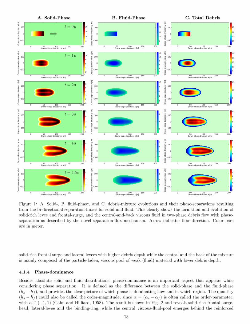
Figure 1: A. Solid-, B. fluid-phase, and C. debris-mixture evolutions and their phase-separations resultingfrom the bi-directional separation-fluxes for solid and fluid. This clearly shows the formation and evolution ofsolid-rich levee and frontal-surge, and the central-and-back viscous fluid in two-phase debris flow with phase-separation as described by the novel separation-flux mechanism. Arrow indicates flow direction. Color barsare in meter.
A. Solid-Phase B. Fluid-Phase C. Total Debris
=⇒t = 0 s
t = 1 s
t = 2 s
t = 3 s
t = 4 s
t = 4.5 s
solid-rich frontal surge and lateral levees with higher debris depth while the central and the back of the mixtureis mainly composed of the particle-laden, viscous pool of weak (fluid) material with lower debris depth.
4.1.4 Phase-dominance
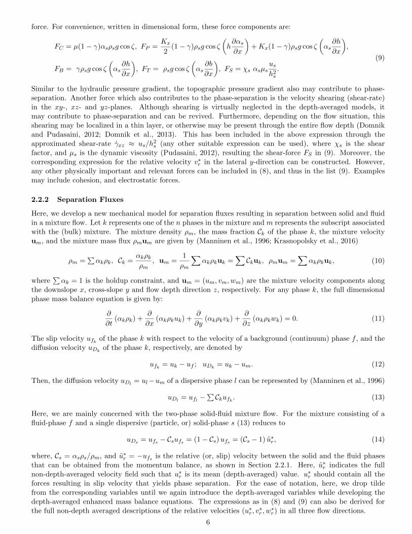
Besides absolute solid and fluid distributions, phase-dominance is an important aspect that appears whileconsidering phase separation. It is defined as the difference between the solid-phase and the fluid-phase(hs − hf ), and provides the clear picture of which phase is dominating how and in which region. The quantity(hs − hf ) could also be called the order-magnitude, since α = (αs − αf ) is often called the order-parameter,with α ∈ (−1, 1) (Cahn and Hilliard, 1958). The result is shown in Fig. 2 and reveals solid-rich frontal surge-head, lateral-levee and the binding-ring, while the central viscous-fluid-pool emerges behind the reinforced
13

Down−slope direction: x [m]
Cro
ss−
slop
e di
rect
ion:
y [m
]
−20 0 20 40 60 80 100 120 140 160 180 200
−150
−100
−50
0
50
100
150
−3
−2
−1
0
1
2
3
Figure 2: Formation of levee and frontal-surge in two-phase debris flow with phase-separation as described bythe novel separation-flux mechanism at time t = 4.5 s. The figure is obtained by subtracting fluid-phase panel(with fluid in the central-back) from the solid-phase panel (with solid-levee and front wall) from Fig. 1. Thefigure shows the solid (in red) - fluid (blue) phase-dominance regions. Color bar is in meter.
solid binding-ring. This is in line with observed phenomena in debris flows (Iverson, 1997; 2003; Fairfield, 2011;Battella et al., 2012; Johnson et al., 2012; Braat, 2014; De Haas et al., 2015).
4.2 Application of the Phase-separation
The evolution of the total debris mass flow dynamics in Fig. 1 shows a strong solid-rich frontal surge head.Taking into account the detailed information of both, the solid and the fluid phases (panels A and B), we cannow determine the strength of the material from its composition and dynamics, i.e., the accurate solid andfluid volume fractions, and their velocities. Thus, the overall strength of the debris mixture is very high in thefrontal region and this strength decreases towards the tail of the debris body.
The detailed information on the evolution and distribution of the flow constituents allows to determine thedynamics and the impacts of the total debris mass. The results in Fig. 1 and Fig. 2 indicate that the overallstrength of the debris mixture is very high in the frontal and lateral regions and decreases in the back side andthe central part of the debris body. Proper knowledge of the dynamics of the phase migration (or, separation)is important, because due to its material composition (e.g., with less bulk density and viscous dissipation) thefluid-rich surge is mechanically much weaker and dynamically less destructive compared to the solid-rich surgesin the frontal head. This information is important to accurately design the defense and impact dissipationstructures in the debris prone regions.
5 Summary
The phase-separation between solid and fluid as a two-phase mass moves down slope is an often observedphenomenon and is a great challenge for scientists and engineers. To address this issue, we proposed a funda-mentally new separation-flux mechanism capable of resolving the strong phase-separation in geophysical massflows such as avalanches or debris flows. This is achieved by extending the general two-phase debris flow model(Pudasaini, 2012) with a separation-flux mechanism. The novel separation-flux model incorporates severaldominant physical and mechanical aspects that result in strong phase-separation. The simulation results showthat the new flux separation mechanism adequately describes and controls the dynamically evolving phase-separation and levee formation in two-phase, geometrically three-dimensional debris flows. As the separationmechanism influences the flow dynamics, solid particles are brought to the flow front and the sides. This resultsin a solid-rich and mechanically strong frontal surge head, and the lateral levees followed by a weaker flow bodyand a viscous fluid dominated tail. These phase-separation phenomena are revealed here for the first time intwo-phase debris flow modeling and simulations. These simulations are in line with the field observations andlaboratory experiments of debris flows.
The in-depth knowledge of the local structural and compositional evolution of the debris mixture together withthe explicit picture of the solid and the fluid phases is very important for the proper understanding of thecomplex debris flow process. The process understanding is required to investigate the mechanical, dynamical,
14
depositional and morphological aspects of the flow that play a vital role in structural engineering of defensestructures and developing proper mitigation plans and hazard assessments in debris flow prone regions. Nottaking into account these effects may result adversely as those structures cannot withstand the impact pressuresexerted by the front that has much larger destructive power than that estimated in a classical fashion by singlephase models, implying an uniform distribution of the composite material through the entire debris body. Fortypical debris flows, the solid density is about a factor three of the fluid material, and factor more than twoof the mixture. Thus, just taking into account the material composition difference (neglecting the differencein the velocity evolution), impact pressure estimates of uniform mixture concepts may appear a factor two toolow. This is of great importance, considering structural design of infrastructure in potentially endangered areasand justifies the application of the present model.
Acknowledgements: This work has been conducted as part of the international cooperation projects: “De-velopment of a GIS-based Open Source Simulation Tool for Modelling General Avalanche and Debris Flowsover Natural Topography (avaflow)” supported by the German Research Foundation (DFG, project numberPU 386/3-1) and the Austrian Science Fund (FWF, project number I 1600-N30).
References
[1] Bathurst, J., A. Burton, T. Ward (1997), Debris flow run-out and landslide sediment delivery modeltests, J. Hydraul. Eng., 123(5), 410-419.
[2] Bartelt, P., and B. W. McArdell (2009), Granulometric investigations of snow avalanches, J. Glaciol.,55(193), 829-833.
[3] Bartelt, P., J. Glover, T. Feistl, Y. Buhler, O. Buser (2012), Formation of levees and en-echelon shearplanes during snow avalanche run-out, Journal of Glaciology, 58, 980-992.
[4] Battella, F., T. Bisantino, V. D’Agostino, F. Gentile (2012), Debris-flow runout distance: laboratoryexperiments on the role of Bagnold, Savage and friction numbers, WIT transactions on EngineeringSciences, 73, 27-36.
[5] Berti, M., and A. Simoni (2007), Prediction of debris flow inundation areas using empirical mobilityrelationships, Geomorphology, 90(1), 144-161.
[6] Braat, L. (2014), Debris flows on Mars: An experimental analysis. Master Thesis, Earth Sciences atUtrecht University, the Netherlands.
[7] Cahn, J. W., and J. E. Hilliard (1958), Free Energy of a Nonuniform System. I. Interfacial Free Energy,The Journal of Chemical Physics 28, 258-267.
[8] Conway, S. J., A. Decaulne, M. R. Balme, J. B. Murray, M. C. Towner (2010), A new approach toestimating hazard posed by debris flows in the Westfjords of Iceland, Geomorphology, 114(4), 556-572.
[9] Costa, J. E. (1988), Rheologic, geomorphic, and sedimentologic differentiation of water flood, hypercon-centrated flows, and debris flows, in Flood Geomorphology, chap. Rheologic, geomorphic, and sedimento-logic differentiation of water floods, hyperconcentrated flows, and debris flows, pp. 113-122, John Wiley,New York.
[10] Crosta, G. B., H. Chen, C. F. Lee (2004), Replay of the 1987 Val Pola Landslide, Italian Alps, Geomor-phology, 60(1-2), 127-146.
[11] D’Agostino, V., M. Cesca, L. Marchi (2010), Field and laboratory investigations of runout distances ofdebris flows in the Dolomites (Eastern Italian Alps), Geomorphology, 115(3), 294-304.
[12] de Haas, T., L. Braat, J. R. F. W. Leuven, I. R. Lokhorst, M. G. Kleinhans (2015), Effects of debris flowcomposition on runout, depositional mechanisms, and deposit morphology in laboratory experiments, J.Geophys. Res. Earth Surf., 120, 1949-1972.
15

[13] Domnik, B., and S. P. Pudasaini (2012), Full two-dimensional rapid chute flows of simple viscoplasticgranular materials with a pressure-dependent dynamic slip-velocity and their numerical simulations, J.Non-Newtonian Fluid Mech., 173, 72-86.
[14] Domnik, B., S. P. Pudasaini, R. Katzenbach, S. A. Miller (2013), Coupling of full two-dimensional anddepth-averaged models for granular flows, J. Non-Newtonian Fluid Mech., 201, 56-68.
[15] Fairfield, G. (2011), Assessing the dynamic influences of slope angle and sediment composition on debrisflow behaviour: An experimental approach, Durham theses, Durham University, 3265.
[16] Felix, G., and N. Thomas (2004), Relation between dry granular flow regimes and morphology of deposits:formation of levees in pyroclastic deposits, Earth Planet. Sci. Lett., 221(1-4), 197-213.
[17] Fischer, J.-T., J. Kowalski, S. P. Pudasaini (2012), Topographic curvature effects in applied avalanchemodeling, Cold Regions Science and Technology, 74-75, 21-30.
[18] Golick, L. A., and K. E. Daniels (2009), Mixing and segregation rates in sheared granular materials,Phys. Rev. E, 80, 042301, doi:10.1103/PhysRevE.80.042301.
[19] Gray, J. M. N. T., and K. Hutter (1997), Pattern formation in granular avalanches, Contin. Mech.Thermodyn., 9, 341-345.
[20] Gray, J. M. N. T., and A. R. Thornton (2005), A theory for particle size segregation in shallow granularfree-surface flows, Proc. R. Soc. A, 461(2057), 1447-1473.
[21] Gray, J. M. N. T., and C. Ancey (2009), Segregation, recirculation and deposition of coarse particles neartwo-dimensional avalanche fronts, J. Fluid Mech., 629, 387-423.
[22] Gray, J. M. N. T., and B. P. Kokelaar (2010), Large particle segregation, transport and accumulation ingranular free-surface flows, J. Fluid Mech., 652, 105-137.
[23] Hillert, M. H. (1956), A theory of nucleation for solid metallic solutions, Massachusetts Institute ofTechnology, USA.
[24] Hurlimann, M., B. W. McArdell, C. Rickli (2015), Field and laboratory analysis of the runout character-istics of hillslope debris flows in Switzerland, Geomorphology, 232, 20-32.
[25] Iverson, R. M. (1997), The physics of debris flows, Rev. Geophys., 35(3), 245-296.
[26] Iverson, R. M., and R. P. Denlinger (2001), Flow of variably fluidized granular masses across three-dimensional terrain: 1. Coulomb mixture theory, J. Geophys. Res., 106(B1), 537-552.
[27] Iverson, R. M., and J. W. Vallance (2001), New views of granular mass flows, Geology, 29(2), 115-118.
[28] Iverson, R. M. (2003), The debris-flow rheology myth, in 3rd International Conference on Debris-FlowHazards Mitigation: Mechanics, Prediction, and Assessment, Ed. by D. Rickenmann, and C. L. Chen,pp. 303-314, Millpress.
[29] Iverson, R. M., M. Logan, R. G. LaHusen, M. Berti (2010), The perfect debris flow? Aggregated resultsfrom 28 large-scale experiments, J. Geophys. Res., 115, F03005, doi:10.1029/2009JF001514.
[30] Johnson, C. G., B. P. Kokelaar, R. M. Iverson, M. Logan, R. G. LaHusen, J. M. N. T. Gray (2012),Grain-size segregation and levee formation in geophysical mass flows, J. Geophys. Res., 117, F01032,doi:10.1029/2011JF002185.
[31] Kafle, J., P. R. Pokhrel, K. B. Khattri, P. Kattel, B. M. Tuladhar, S. P. Pudasaini (2016), Landslide-generated tsunami and particle transport in mountain lakes and reservoirs, Annals of Glaciology, 71,http://dx.doi.org/10.3189/2016AoG71A034.
16

[32] Kattel, P., K. M. Khattri, P. R. Pokhrel, J. Kafle, B. M. Tuladhar, S. P. Pudasaini (2016), Sim-ulating glacial lake outburst floods with a two-phase mass flow model. Annals of Glaciology, 71,http://dx.doi.org/10.3189/2016AoG71A039.
[33] Kern, M., O. Buser, J. Peinke, M. Siefert, L. Vulliet (2005), Stochastic analysis of single particle segre-gational dynamics, Physics Letters A, 336(4-5), 428-433.
[34] Krasnopolsky, B., Starostin, A., Osiptsov, A. A. (2016), Unified graph-based multi-fluid model for gasliq-uid pipeline flows, Computers and Mathematics with Applications, 72, 1244-1262.
[35] Major, J. J., and R. M. Iverson (1999), Debris-flow deposition: Effects of pore-fluid pressure and frictionconcentrated at flow margins, Geol. Soc. Am. Bull., 111(10), 1424-1434.
[36] Manninen, M, V. Taivassalo, S. Kallio (1996), On the mixture model for multiphase flow, Espoo, TechnicalResearch Center of Finland, VTT Publications 228 (ISBN 951-38-4946-5; ISSN 1235-0621).
[37] McArdell, B. W., P. Bartelt, J. Kowalski (2007), Field observations of basal forces and fluid pore pressurein a debris flow, Geophys. Res. Lett., 34, L07406, doi:10.1029/2006GL029183.
[38] Mergili, M., K. Schratz, A. Ostermann, W. Fellin (2012), Physically-based modelling of granular flowswith Open Source GIS, Nat. Hazards Earth Syst. Sci., 12, 187-200.
[39] Pierson, T. C. (2005), Distinguishing Between Debris Flows and Floods From Field Evidence in SmallWatersheds, US Dep. of the Int., U.S. Geol. Survey, Reston, Va.
[40] Pirulli, M. (2009), The Thurwieser rock avalanche (Italian Alps): Description and dynamic analysis, Eng.Geol., 109, 80-92.
[41] Pitman, E. B., and L. Le (2005), A two-fluid model for avalanche and debris flows, Philos. Trans. R. Soc.A, 363, 1573-1602.
[42] Pouliquen, O., J. Delour, S. B. Savage (1997), Fingering in granular flows, Nature, 386, 816-817.
[43] Pudasaini, S. P., Y. Wang, K. Hutter (2005), Modelling debris flows down general channels, Nat. HazardsEarth Syst. Sci., 5, 799-819.
[44] Pudasaini, S. P., and K. Hutter (2007), Avalanche Dynamics: Dynamics of Rapid Flows of Dense GranularAvalanches, 602 pp., Springer, New York.
[45] Pudasaini, S. P. (2012), A general two-phase debris flow model, J. Geophysics. Res., 117, 2012. F03010,doi:10.1029/ 2011JF002186.
[46] Pudasaini, S. P., and S. A. Miller (2013), The hypermobility of huge landslides and avalanches, Eng.Geol., 157, 124-132.
[47] Pudasaini, S. P. (2014), Dynamics of submarine debris flow and tsunami, Acta Mech., 225, 2423-2434.
[48] Pudasaini, S. P., and M. Krautblatter (2014), A two-phase mechanical model for rock-ice avalanches, J.Geophys. Res. Earth Surf., 119, doi:10.1002/2014JF003183.
[49] Pudasaini, S. P. (2015), A novel mechanical model for phase-separation in debris flows, GeophysicalResearch Abstracts, 17, EGU2015-2915.
[50] Rickenmann, D. (1999), Empirical relationships for debris flows, Nat. Hazards, 19(1), 47-77.
[51] Rickenmann, D. (2005), Debris-Flow Hazards and Related Phenomena, chap. Runout Prediction Meth-ods, pp. 305-324, Praxis, Chichester, U. K.
[52] Savage, S. B., and C. K. K. Lun (1988), Particle size segregation in inclined chute flow of dry cohesionlessgranular solids, J. Fluid Mech., 189, 311-335.
17

[53] Schneider, D., C. Huggel, W. Haeberli, R. Kaitna (2011), Unraveling driving factors for large rock-iceavalanche mobility, Earth Surf. Processes Landforms, 36(14), 1948-1966.
[54] Sharp, R. P., and L. Nobles (1953), Mudflow of 1941 at Wrightwood, southern California, Geol. Soc. Am.Bull., 64(5), 547-560.
[55] Shearer, M., J. M. N. T. Gray, A. R. Thornton (2008), Stable solutions of a scalar conservation law forparticle-size segregation in dense granular avalanches, Eur. J. Appl. Math., 19, 61-86.
[56] Scheidl, C., and D. Rickenmann (2010), Empirical prediction of debris-flow mobility and deposition onfans, Earth Surf. Process. Landforms, 35(2), 157-173.
[57] Steinkogler, W., J. Gaume, H. Lowe, B. Sovilla, M. Lehning (2015), Granulation of snow: From tum-bler experiments to discrete element simulations, Journal of Geophysical Research: Earth Surface,120(6):1107-1126.
[58] Takahashi, T. (1991), Debris Flow, Balkema, Rotterdam, Netherlands.
[59] Tai, Y. C., S. Noelle, J. M. N. T. Gray, K. Hutter (2002), Shock-capturing and front tracking methodsfor granular avalanches, J. Comput. Phys., 175, 269-301.
[60] Vladimirova, N., A. Malagoli, R. Mauri (1999), Two-dimensional model of phase segregation in liquidbinary mixtures, Physical Review E, 60, 6968-6977.
[61] Wiederseiner, S., N. Andreini, G. Epely-Chauvin, G. Moser, M. Monnereau, J. M. N. T. Gray, C. Ancey(2011), Experimental investigation into segregating granular flows down chutes, Phys. Fluids, 23, 013301,doi:10.1063/1.3536658.
18


![Obracania 2D Autodesk Mechanical Simulation · 2020-04-13 · 9x[sv^irmi fv]] pyf ipiqirxy ow^xexyngiks tv^i^ []gmkrmgmi tvswxi xs reng^gmin []osv^]wx][eri rev^h^mi ow^xexs[erme 3tivegne](https://img.dokumen.tips/doc/110x75/5f94ab12aec36a57fc0ef22a/obracania-2d-autodesk-mechanical-simulation-2020-04-13-9xsvirmi-fv-pyf-ipiqirxy.jpg)