A Matlab And Simulink Based Software Environment For

Document: 2004--826

A MATLAB/SIMULINK BASED ENVIRONMENT FOR INTELLIGENT MODELLING

AND SIMULATION OF FLEXIBLE MANIPULATOR SYSTEMS

Abul K M Azad*, M. O. Tokhi§, A. Pathania

*, and M. H. Shaheed

+

* Department of Technology, Northern Illinois University, IL-60115, USA. § Department of Automatic Control and Systems Engineering, University of Sheffield, UK.

+ Department of Engineering, Queen Mary, University of London, London, UK.

1. Introduction

Flexible manipulator systems are receiving increasing attention due to their advantages over

conventional robot manipulators. The advantages include faster response, lower energy

consumption, relatively smaller actuators, higher payload to weight ratio and, in general, less

overall cost 1. Some of the current applications of such manipulators include spacecraft, remote

manipulation and radioactive material handling in nuclear power plants. Due to their flexible

nature, induced vibrations appear in the system during and after a positioning motion 2,3

. This

restricts their wide spread use in industry. A considerable amount of research work has already

been carried out on the vibration control of flexible manipulators. However, a generic solution to

the problem is yet to be obtained 4,5

.

To formulate and implement an effective control strategy for efficient vibration suppression of

the system, it is important to recognise the flexible nature of the manipulator and construct a

mathematical model for the system that accounts for the interactions with actuators and payload 6. Such a model can be constructed using partial differential equations (PDEs). The finite element

(FE) and finite difference (FD) methods have also been utilised to describe the flexible behaviour

of manipulators 7. The computational complexity and consequent software coding involved in

the FE method is a major disadvantage of this technique 8. An alternative solution is to utilise

intelligent techniques, such as genetic algorithms (GAs) and neural networks (NNs) for

modelling of flexible manipulator systems 9.

The approaches indicated above have proved to be effective in modelling and simulation of such

systems for test and verification of controller designs. However, to allow interactive and user

friendly features, that are desired especially in computer aided teaching and research, be

incorporated a modelling, simulation and control environment is developed in this work for

flexible manipulators using Matlab and Simulink. To this end the authors have developed an

interactive and user-friendly environment referred to as SCEFMAS (Simulation and Control

Environment of Flexible Manipulator Systems) 10

. As an on-going development process, the

SCEFMAS environment is enhanced by the addition of intelligent modelling, a new menu driven

user interface with GUI based facility, and the display of results within the GUI facility.

Moreover, the environment is upgraded from Matlab 4.2 to Matlab 6.5. This paper describes

these recent developments in SCEFMAS. The rest of the paper is structured as follows: Section 2

Proceedings of 2004 American Society for Engineering Education Annual Conference & Exposition

Copyright @2004, American Society for Engineering Education

Page 9.62.1

briefly describes the flexible manipulator system considered and the corresponding FD

simulation process. Section 3 illustrates the GA and NN modelling strategies. Section 4 describes

the implementation of the FD simulation algorithm, GA and NN modelling strategies within the

SCEFMAS framework. The developed GUIs are also described in this section. The paper is

concluded in Section 5.

2. The Flexible Manipulator System

The flexible manipulator system under consideration is modelled as a pinned-free flexible beam,

with a mass at the hub, which can bend freely in the horizontal plane but is stiff in vertical

bending and torsion. The model development utilises the Lagrange equation and modal

expansion method 11,12

. To avoid the difficulties arising due to time varying length, the length of

the manipulator is assumed to be constant.

X0

Y0

X

s*t+

Flexible Link ( t."E."I, L )

v

Y

Rigid Hub ( Ih )

w*x,t+

mp

O

x

Figure 1: Schematic representation of the flexible manipulator system.

A schematic representation of the manipulator is shown in Figure 1, where and

represent the stationary and moving co-ordinate frames respectively. The axis coincides

with the neutral line of the link in its undeformed configuration, and is tangent to it at the

clamped end in a deformed configuration. The represents the applied torque at the hub. , ,

, , and represent the Young modulus, area moment of inertia, mass density per unit

volume, cross sectional area, hub inertia and payload of the manipulator respectively.

denotes an angular displacement (hub-angle) of the manipulator and denotes an

elastic deflection (deformation) of a point along the manipulator at a distance from the hub of

the manipulator. In this work, the motion of the manipulator is confined to the plane.

The width of the arm is assumed to be much greater than its thickness, thus, allowing the

manipulator to vibrate (be flexible) dominantly in the horizontal direction. The shear

deformation and rotary inertia effects are also ignored.

ooOYX

OX

),( txw

x

oX

XOY

Ev I

t S I m

t

OY

h p

)(s

o

To obtain equations of motion of the manipulator, the associated energies have to be obtained.

These include the kinetic, potential and dissipated energies. Thus, using the Hamilton’s extended

method, a partial differential equation (PDE) describing the dynamic equation of the flexible

manipulator with associated boundary and initial conditions can be obtained 2. The PDE thus



Page 9.62.2

obtained is of a hyperbolic type and can be classified as a boundary value problem. This can be

solved using an FD method 7. This involves dividing the arm into a finite number of equal-length

sections and developing a linear difference equation describing the deflection of end of each

section (grid-point). Thus, using the FD method, a solution of the PDE can be obtained and

implemented on a digital processor 2

.

3 Intelligent Modelling

In many cases, when it is difficult to obtain a model structure for a system with traditional

system identification techniques, intelligent techniques are desired that can describe the system

in the best possible way 9. GAs and NNs are two intelligent techniques used commonly for

system identification and modelling. The major advantage of utilising GAs for system

identification is that GAs simultaneously evaluates many points in the parameter space and

converge towards the global solution 13

. The superiority of a GA over recursive least squares

(RLS) algorithm in modelling a fixed-free flexible beam is addressed by 14

. In contrast, NN

approaches for system identification offer many advantages over traditional ones especially in

terms of flexibility and hardware realisation 15

. This technique is quite efficient in modelling

non-linear systems or if the system possesses nonlinearities to any degree.

Once a model of the system is obtained, it is required to validate whether the model is good

enough to represent the system. A number of such validation tests are available in the literature 15

. These are one-step ahead (OSA) prediction; model predicted output (MPO), and correlation

tests. Such techniques are incorporated within SCEFMAS for validating developed models.

Moreover, with NN modelling, the input-output data set is divided into two halves. The first half

is used to train the NN and the output computed. The NN usually tracks the system output well

and converges to a suitable error minimum. New inputs are presented to the trained neural

network and the predicted output is observed. If the fitted model is correct, i.e., correct

assignment of lagged inputs and outputs, then the network will predict well for the prediction set.

In this case the model will have captured the underlying dynamics of the system. If both the OSA

and the MPO of a fitted model are good over the estimation and prediction data sets then most

likely the model is unbiased.

3.1 GA Modelling

With GA modelling an initial population of potential solutions is created in the first step. Each

element of the population is mapped onto a set of strings (the chromosome) to be manipulated by

the genetic operators. In the second step, the performance of each member of the population is

assessed through an objective function imposed by the problem. This establishes the basis for

selection of pairs of individuals that will be mated together during reproduction. For

reproduction, each individual is assigned a fitness value derived from its raw performance

measure, given by the objective function. This value is used in the selection to bias towards more

fit individuals. Highly fit individuals, relative to the whole population, have a high probability of

being selected for mating, whereas less fit individuals have a correspondingly low probability of

being selected 16

.

In the manipulation phase, genetic operators such as crossover and mutation are used to produce

a new population of individuals (offspring) by manipulating the genetic information usually



Page 9.62.3

called genes, possessed by the members (parents) of the current population. The crossover

operator is used to exchange genetic information between pairs, on larger groups, of individuals.

Mutation is generally considered to be a background operator, which ensures that the search

process is not trapped at local minimum, by introducing new genetic structures in the population.

After manipulation by the crossover and mutation operators, the individual strings are then, if

necessary, decoded, the objective function evaluated, a fitness value assigned to each individual

and individuals selected for mating according to their fitness, and so the process continues

through subsequent generations. In this way, the average performance of individuals in a

population is expected to increase, as good individuals are preserved and breed with one another

and the less fit individuals die out. The GA is terminated when some criteria are satisfied, e.g., a

certain number of generations completed or when a particular point in the search space is

reached.

For parametric identification of the manipulator with GA, randomly selected parameters are

optimised for different, arbitrarily chosen order to fit to the system by applying the working

mechanism of GA as described above. The fitness function utilised is the sum-squared error

between the actual output, , of the system and the predicted output, , produced from

the input to the system and the optimised parameters:

y n( ) #( )y n

* +f e y n y ni

n

( ) ( ) #( )? /?Â 2

1

Where, is the number of input/output samples. With the fitness function given above, the

global search technique of the GA is utilised to obtain the best set of parameters among all the

attempted orders for the system. The output of the system is thus simulated using the best sets of

parameters and the system input.

n

3.2 NN Modelling

Various modelling techniques can be used with neural networks to identify a non-linear

dynamical system. These include state-output model, recurrent state model and non-linear

autoregressive moving average process with exogeneous (NARMAX) input model. However,

from the literature it has been established that if the plant’s input and output data are available,

the NARMAX model is a suitable choice, for modelling systems with nonlinearities.

Mathematically, the model is given as 17

:

)()]( , ),2(e ),1(

),( , ),2( ),1(

),( , ),2( ),1([()(ˆ

tentette

ntututu

ntytytyfty

e

u

y

-//////

///?

5

5

5

Where, is the output vector determined by the past values of the system input vector, output

vector and noise with maximum lags , and respectively, is the system mapping

constructed through multilayer perceptron (MLP) or radial basis function (RBF) neural networks

with an appropriate learning algorithm. The model is also known as NARMAX equation error

model. However, if the model is good enough to identify the system without incorporating the

)(ˆ ty

yn n n )(©fu e



Page 9.62.4

noise term or considering the noise as additive at the output the model can be represented in a

NARX form 17,18

as:

)()]( , ),2( ),1(

),( , ),2( ),1([()(ˆ

tentututu

ntytytyfty

u

y

-///

///?

5

5

With both GA and NN modelling the manipulator is modelled from the input torque to hub-

angle, hub-velocity and end-point acceleration. These are referred to as the hub-angle model,

hub-velocity model and end-point acceleration model respectively.

4. SCEFMAS Environment

A major portion of the initial version of the SCEFMAS was developed using Simulink 10

.

Moreover, SCEFMAS utilizes the Matlab Guide (GUI development tool) for the development of

GUIs 19,20

. The working principle of the SCEFMAS is shown by a flow-chart in Figure 2.

Figure 2: Flow-chart of the SCEFMAS environment.

The Initial GUI allows the user to provide the flexible manipulator specifications, material

properties and simulation parameters. Following this the user will have the option to choose

algorithm type for simulation and model type. The choices are: FD simulation, GA modelling,

NN modelling.

4.1 Initial GUI

The initial GUI is named as Scefmas_V2 and is used as gateway to the SCEFMAS environment

(Figure 3). Through this GUI the user will have the choice to provide three sets of parameters.

These are Manipulator Specifications, Material Properties, and Simulation Parameters.

Manipulator parameters involve the length, thickness and width of the manipulator along with



Page 9.62.5

the hub inertia and payload. While the material properties constitute damping factor, young’s

modulus and mass density per volume. Finally, the total simulation time, number of segments,

and stability factor for the FD algorithm constitute the simulation parameters. The user then

needs to choose the type of algorithm options from the bottom right side box of the GUI window.

The options are: FD Simulation, NN Modelling or GA Modelling.

Figure 3: Startup GUI for the SCEFMAS environment.

At the bottom of the option selection box there are two radio buttons, which can be used to select

excitation input of the flexible manipulator. The inputs are Random input and Composite PRBS

input. Both of these inputs provide sufficient excitation for all the modes associated with a

flexible manipulator system within the frequency range of excitation.

5.2 FD Simulation and display of results

Once the user clicks on the FD Simulation button within the Scefmas_V2 GUI, the user has the

option of either opening a pre-developed model or one of their own models. Figure 4 shows such

a pre-developed model with a flexible manipulator connected to a random input in an open-loop

manner. The Auxiliary block within the model produces data set for 3D plot within the Result

GUI. After a simulation run the input and outputs are passed to the Matlab environment through

the yin and yout blocks.



Page 9.62.6

Figure 4: Excitation of a flexible manipulator using a random input.

Figure 5: Displaying the results obtained from FD Simulation

At the end of the simulation, a button called Results will be displayed within the Initial GUI

(Figure 3). A click on this button will open a new GUI called Results, which can be used to

display all the input and outputs produced through this simulation process (Figure 5).

The left hand side of the GUI includes option buttons, top right side contains time domain and

frequency domain result windows for the selected input or output parameter, bottom middle

window is for displaying 3D plot of the complete motion of the manipulator for a given

simulation. The drop down menus at the bottom right side can be used to choose properties of the

3D plot. After viewing the result, the user can choose to return to the Initial GUI by clicking on

the New Simulation button or may exit SCEFMAS by clicking on the Quit button within the

Results GUI. The complete FD simulation and display process can be presented through the

flowchart shown in Figure 6. Within the flowchart Simulink Controller is shown as a part of

SCEFMAS and has been reported earlier 10

.



Page 9.62.7

Figure 6: FD simulation flowchart.

4.3 Neural network modelling

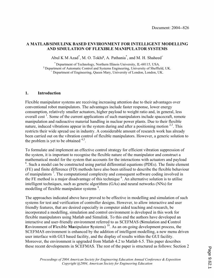
The NN_template GUI, shown in Figure 7 is used for NN modelling of the flexible manipulator

systems. The process starts by clicking on the NN Modelling button within the Scefmas_V2

GUI. The upper part of this window allows the user to choose the number of layers of neurons

within the NN structure along with the property of neurons in each layer. At this point the user

needs to generate the training data for NN modelling. The process starts by clicking on the

Generate Data Set button. The user can choose from a set of FD Models available within the

SCEFMAS environment. At the end of FD simulation the user can view the generated data for

quality assurance. To start the NN training one has to click on the Train Network button at the

bottom middle part of the GUI. This will start the training process and the sum-squared error

will be displayed in a graphical window at the bottom left corner of the GUI. At the end of the

training Simulation Done message will pop up at bottom right corner of the GUI. A new button

called Validation Plots will also appear just below the Train Network button.



Page 9.62.8

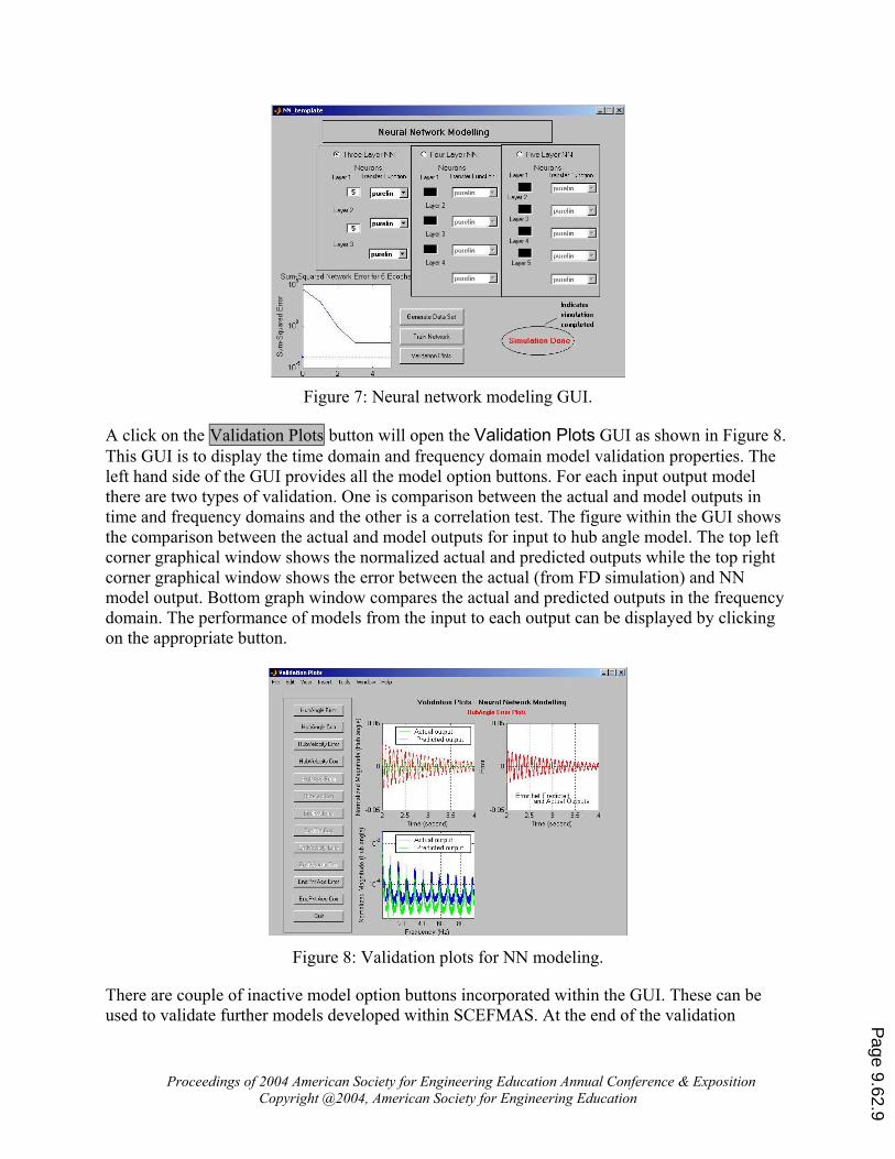
Figure 7: Neural network modeling GUI.

A click on the Validation Plots button will open the Validation Plots GUI as shown in Figure 8.

This GUI is to display the time domain and frequency domain model validation properties. The

left hand side of the GUI provides all the model option buttons. For each input output model

there are two types of validation. One is comparison between the actual and model outputs in

time and frequency domains and the other is a correlation test. The figure within the GUI shows

the comparison between the actual and model outputs for input to hub angle model. The top left

corner graphical window shows the normalized actual and predicted outputs while the top right

corner graphical window shows the error between the actual (from FD simulation) and NN

model output. Bottom graph window compares the actual and predicted outputs in the frequency

domain. The performance of models from the input to each output can be displayed by clicking

on the appropriate button.

Figure 8: Validation plots for NN modeling.

There are couple of inactive model option buttons incorporated within the GUI. These can be

used to validate further models developed within SCEFMAS. At the end of the validation



Page 9.62.9

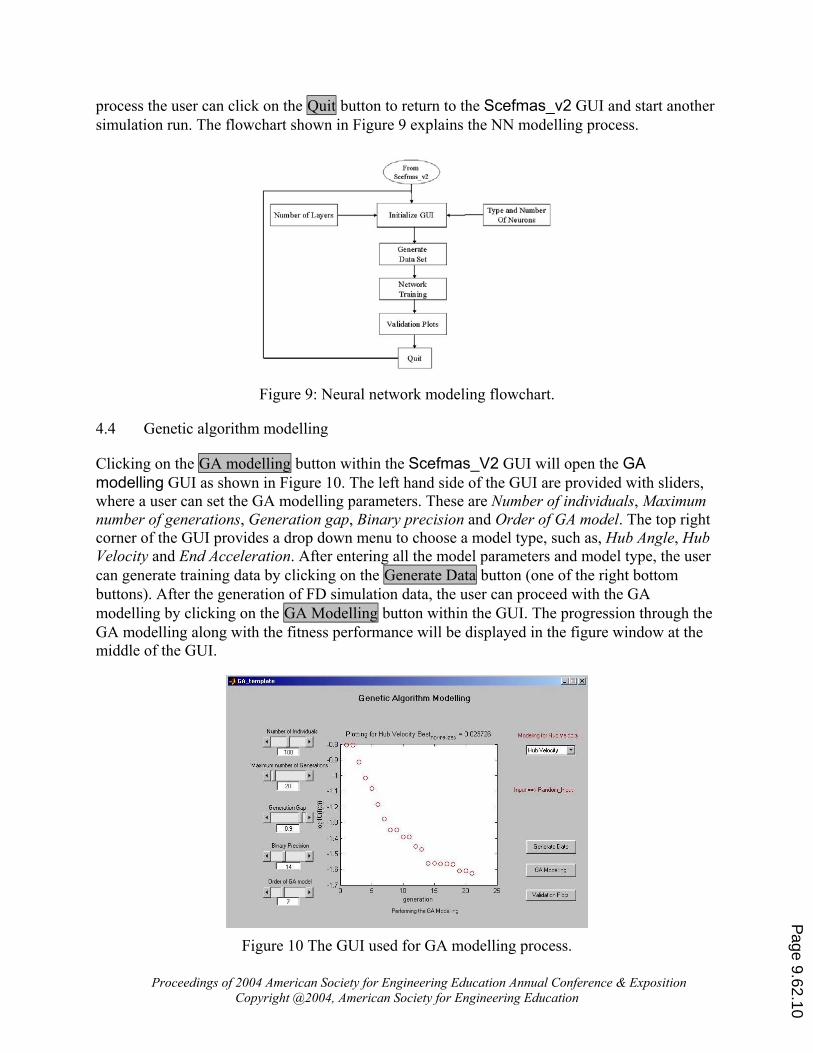
process the user can click on the Quit button to return to the Scefmas_v2 GUI and start another

simulation run. The flowchart shown in Figure 9 explains the NN modelling process.

Figure 9: Neural network modeling flowchart.

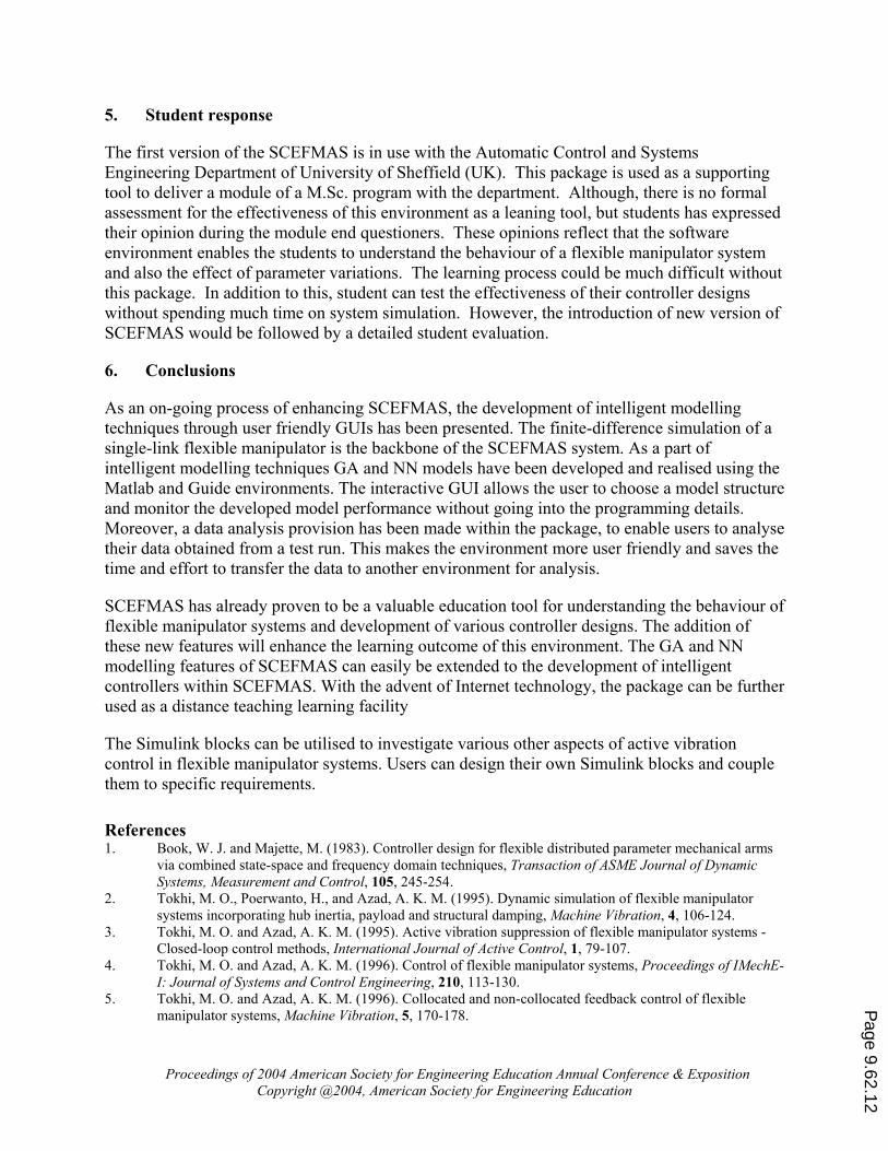
4.4 Genetic algorithm modelling

Clicking on the GA modelling button within the Scefmas_V2 GUI will open the GA

modelling GUI as shown in Figure 10. The left hand side of the GUI are provided with sliders,

where a user can set the GA modelling parameters. These are Number of individuals, Maximum

number of generations, Generation gap, Binary precision and Order of GA model. The top right

corner of the GUI provides a drop down menu to choose a model type, such as, Hub Angle, Hub

Velocity and End Acceleration. After entering all the model parameters and model type, the user

can generate training data by clicking on the Generate Data button (one of the right bottom

buttons). After the generation of FD simulation data, the user can proceed with the GA

modelling by clicking on the GA Modelling button within the GUI. The progression through the

GA modelling along with the fitness performance will be displayed in the figure window at the

middle of the GUI.

Figure 10 The GUI used for GA modelling process.



Page 9.62.10

Figure 11: GA modeling validation GUI.

After the completion of the modelling process the Validation Plots button will be activated

(bottom right corner of the GUI). The user can click on this button to observe the performance of

the developed GA model through GA_Validation_plots GUI (Figure 11). The left hand side of

the GUI is provided with buttons for choosing model types. The model validation outputs are

displayed through four figure windows. Top two figure windows are for comparing the

magnitudes of actual and predicted outputs. The bottom right window shows the comparison

between actual and predicted outputs in the frequency domain. The bottom left window shows

the sum-squared error for each generation. At the end of the GA model validation process the

user can return to the Scefmas_V2 GUI for further modelling exercises. The GA modelling

process is illustrated by the flowchart in Figure 12.

Figure 12: Genetic algorithm modeling flowchart.



Page 9.62.11

5. Student response

The first version of the SCEFMAS is in use with the Automatic Control and Systems

Engineering Department of University of Sheffield (UK). This package is used as a supporting

tool to deliver a module of a M.Sc. program with the department. Although, there is no formal

assessment for the effectiveness of this environment as a leaning tool, but students has expressed

their opinion during the module end questioners. These opinions reflect that the software

environment enables the students to understand the behaviour of a flexible manipulator system

and also the effect of parameter variations. The learning process could be much difficult without

this package. In addition to this, student can test the effectiveness of their controller designs

without spending much time on system simulation. However, the introduction of new version of

SCEFMAS would be followed by a detailed student evaluation.

6. Conclusions

As an on-going process of enhancing SCEFMAS, the development of intelligent modelling

techniques through user friendly GUIs has been presented. The finite-difference simulation of a

single-link flexible manipulator is the backbone of the SCEFMAS system. As a part of

intelligent modelling techniques GA and NN models have been developed and realised using the

Matlab and Guide environments. The interactive GUI allows the user to choose a model structure

and monitor the developed model performance without going into the programming details.

Moreover, a data analysis provision has been made within the package, to enable users to analyse

their data obtained from a test run. This makes the environment more user friendly and saves the

time and effort to transfer the data to another environment for analysis.

SCEFMAS has already proven to be a valuable education tool for understanding the behaviour of

flexible manipulator systems and development of various controller designs. The addition of

these new features will enhance the learning outcome of this environment. The GA and NN

modelling features of SCEFMAS can easily be extended to the development of intelligent

controllers within SCEFMAS. With the advent of Internet technology, the package can be further

used as a distance teaching learning facility

The Simulink blocks can be utilised to investigate various other aspects of active vibration

control in flexible manipulator systems. Users can design their own Simulink blocks and couple

them to specific requirements.

References 1. Book, W. J. and Majette, M. (1983). Controller design for flexible distributed parameter mechanical arms

via combined state-space and frequency domain techniques, Transaction of ASME Journal of Dynamic

Systems, Measurement and Control, 105, 245-254.

2. Tokhi, M. O., Poerwanto, H., and Azad, A. K. M. (1995). Dynamic simulation of flexible manipulator

systems incorporating hub inertia, payload and structural damping, Machine Vibration, 4, 106-124.

3. Tokhi, M. O. and Azad, A. K. M. (1995). Active vibration suppression of flexible manipulator systems -

Closed-loop control methods, International Journal of Active Control, 1, 79-107.

4. Tokhi, M. O. and Azad, A. K. M. (1996). Control of flexible manipulator systems, Proceedings of IMechE-

I: Journal of Systems and Control Engineering, 210, 113-130.

5. Tokhi, M. O. and Azad, A. K. M. (1996). Collocated and non-collocated feedback control of flexible

manipulator systems, Machine Vibration, 5, 170-178.



Page 9.62.12

6. Tse, F. S., Morse, I. E., and Hinkle, T. R. (1980). Mechanical Vibrations Theory and Applications, Allyn

and Bacon Inc.

7. Azad, A. K. M. (1994). Analysis and design of control mechanisms for flexible manipulator systems, PhD

Thesis, University of Sheffield, Department of Automatic Control and Systems Engineering.

8. Kourmoulis, P. K. (1990). Parallel processing in the simulation and control of flexible beam structures,

PhD Thesis, University of Sheffield, Department of Automatic Control and Systems Engineering.

9. Elanayar, S. V. T. and Yung, C. S., (1994). Radial basis function neural network for approximation and

estimation of non-linear stochastic dynamic systems, The IEEE Transaction on Neural Networks, 5, (4), pp.

594-603.

10. Tokhi, M. O., Azad, A. K. M., and Poerwanto, H. (1999). SCEFMAS: A Simulink environment for

dynamic characterisation and control of flexible manipulators, International Journal of Engineering

Education, 15(3), pp. 213-226.

11. Hastings ,G. S. and Book , W. J. (1987). A Linear dynamic model for flexible robotic manipulator, IEEE

Control Systems Magazine, 7, pp. 61-64.

12. Korolov, V. V. and Chen,Y. H. (1989). Controller design robust to frequency variation in a one-link

flexible robot arm, Journal of Dynamic Systems, Measurement and Control, 111, pp. 9-14.

13. Kristinsson, K. and Dumont, G. (1992). System identification and control using genetic algorithms, The

IEEE Transactions on Systems, Man and Cybernetics, 22, (5), pp. 1033-1046.

14. Hossain, M. A., Tokhi, M. O., Chipperfield, A. J., Fonseca, C. M., and Dakev, N. V. (1995). Adaptive

active vibration control using genetic algorithms. The 1st IEE/IEEE International Conference on GAs in

Engineering Systems: Innovations and Applications, Sheffield, UK, pp. 175-180.

15. Ljung, L. and Sj berg, J. (1992). A system identification perspective on neural networks. Neural

Networks for Signal Processing II.-Proceedings. of the IEEE-SP Workshop, Helsingoer, Denmark, pp. 423-

435.

%%o

16. Chipperfield, A. J. and Fleming, P. J. (1994). Parallel Genetic Algorithms: A Survey, Research report no.

518, Department of Automatic Control and Systems Engineering, The University of Sheffield, UK.

17. Luo, F-L. and Unbehauen, R. (1997). Applied neural networks for signal processing. Cambridge University

Press, Cambridge, New York.

18. Sze, T. L. (1995). System identification using radial basis neural networks, PhD thesis, Department of

Automatic Control and Systems Engineering, The University of Sheffield, Sheffield, UK.

19. The Mathworks Inc, MATLAB Guide Users Manual, The Mathworks Inc. Natwick (2002).

20. The Mathworks Inc, SIMULINK, Users Guide, The Mathworks Inc. Natwick (2001).

BIOGRAPHICAL INFORMATION

ABUL K M AZAD

Obtained PhD (control engineering) from the University of Sheffield (UK) in 1994. He is now an Assistant

Professor with the Engineering Technology Department of NIU. Dr Azad has over 50 papers in this area and is

active with professional bodies. His current teaching and research interests include digital electronics, mechatronics,

intelligent control and real-time computer control of engineering systems.

M. O. TOKHI

Osman Tokhi obtained his BSc (Electrical Engineering) from Kabul University (Afghanistan) in 1978 and PhD from

Heriot-Watt University (UK) in 1988. He has worked at various academic and industrial establishments since

graduation in 1978, and is currently employed as Reader in the Department of Automatic Control and Systems

Engineering, The University of Sheffield (UK). His research interests include active noise and vibration control,

real-time signal processing and control, system identification and adaptive/intelligent control, biomedical

applications of robotics and control. He has active membership and involvement in several learned societies

including the IEE, IEEE and the IIAV.

M. H. SHAHEED

Lecturer in Robotics, Control and Computing, Department of Engineering, Queen Mary, University of London, UK.

He completed his PhD (Control Engineering) from the University of Sheffield in 2000. His research interests include



Page 9.62.13

system identification and control using model-based and AI-based approaches and high performance computing. He

has been able to publish several refereed journals and conference papers. He is a member of both IEE and IEEE.

AMIT PATHANIA

Amit is presently a graduate student in the Department of Electrical Engineering at Northern Illinois University. He

has his B.Engg. in Electronics and Telecommunication from the Bhilai Institute of Technology, India. In his MS

course at the NIU, Amit had course in DSP, Digital communication, Robotics and Neural networks. His interests are

in the areas of communications and software development.



Page 9.62.14

Documents

A Matlab And Simulink Based Software Environment For