TitleA Mathematical Note on the Feynman Path Integral for theQuantum Electrodynamics(Spectral and Scattering Theory andRelated Topics)

Author(s) ICHINOSE, Wataru

Citation 数理解析研究所講究録 (2007), 1563: 52-68

Issue Date 2007-06

URL http://hdl.handle.net/2433/81124

Right

Type Departmental Bulletin Paper

Textversion publisher

Kyoto University

A Mathematical Note on the Feynman Path Integral for the

Quantum Electrodynamics

信州大学理学部 一ノ瀬 弥 1 (Wataru ICHINOSE)

Department of Mathematical Science, Shinshu University, Matsumoto

390-8621, Japan. E-mail: ichinose@@math.shinshu-u.ac.jp

1 Introduction.

A number of mathematical results on the Feynman path integral for the

quantum mechanics have been obtained. On the other hand, the author doesn’t

know any mathematical results on the Feynman path integral for the quantum

electrodynamics, written as QED from now on. A functional integral repre-

sentation for a non-relativistic QED model with imaginary time was obtained

by Hiroshima (1997) [7] by means of the probabilistic method.

Our aim in the present paper is to give the mathematical definition of the

Feynman path integral for the non-relativistic QED, especially studied in Feyn-

man (1950) [4] and Feynman - Hibbs (1965) [5]. In the present paper the

Fourier series is used as in Fermi (1932) [2], Feynman [4] and Sakurai (1967)

[13], and photons with large momentum are arbitrarily cut off.

We first give the mathematical definition of the Feynman path integral for

the non-relativistic QED under the constraint condition, whose method is well

$lResearch$ partially supportteedd by Grant-in-Aid for Scientific No.16540145, Ministry of

Education, Science, and Culture, Japanese Government.

数理解析研究所講究録第 1563巻 2007年 52-68 52

known (cf. (9.7) in [5], (A-7) in [13], (13.10) in Spohn (2004) [14] and (7.38) in

Swanson (1992) [15]). Secondly, without the constraint condition we give the

mathematical definition of the Feynman path integral for the non-relativistic

QED, which is given by (9-98) in [5]. The author emphasize that any concrete

definition of (9-98) in [5] is not given. So our result may be completely new.

We also note that our Feynman path integral without the constraint condition

is proved to be equal with the Feynman path integral under the constraint

condition.

Our plan in the present paper is as follows. \S 2 is devoted to preliminaries.

In \S 3 we give the mathematical definition of the Feynman path integral for

the non-relativistic QED under the constraint condition and prove that this

Feynman path integral converges. We also state some remarks. In particular,

the expressions of the Hamiltonian operator and etc. by means of the creation

operators and the annihilation operators are given in Remark 3.3. These ex-

pressions are used in many literatures (cf. Gustafson-Sigal (2003) [6], [7], [13]

and [14]). In \S 4 we give the mathematical definition of the Feynman path in-

tegral for the non-relativistic QED without the constraint condition and prove

that our Feynman path integral without the constraint condition is equal to

the Feynman path integral under the constraint condition. So, the Feynman

path integral without the constraint condition is also proved to converge from

the result in \S 3.

53

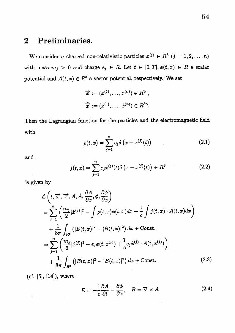
2 Preliminaries.

We consider $n$ charged non-relativistic particles $x^{(j)}\in R^{3}(j=1,2, \ldots, n)$

with mass $m_{j}>0$ and charge $e_{j}\in R$ . Let $t\in[0,T],$ $\phi(t, x)\in R$ a scalar

potential and $A(t, x)\in R^{3}$ a vector potential, respectively. We set

$?:=(x^{(1)}, \ldots, x^{(n)})\in R^{3n}$ ,

$\ovalbox{\tt\small REJECT}$ $:=(\dot{x}^{(1)}, \ldots,\dot{x}^{(n)})\in R^{3n}$ .

Then the Lagrangian function for the particles and the electromagnetic field

with

$p(t, x)= \sum_{j=1}^{n}e_{j}\delta(x-x^{(j)}(t))$ (2.1)

and

$j(t, x)= \sum_{j=1}^{n}e_{j}\dot{x}^{(j)}(t)\delta(x-x^{(j)}(t))\in R^{3}$ (2.2)

is given by

$\mathcal{L}(t,$ $i,$ $?,$ $A,\dot{A},$ $\frac{\partial A}{\partial x},$ $\phi,$ $\frac{\partial\phi}{\partial x})$

$= \sum_{j=1}^{n}(\frac{m_{j}}{2}|\dot{x}^{(j)}|^{2}-\int\rho(t, x)\phi(t,x)dx+\frac{1}{c}\int j(t, x)\cdot A(t, x)dx)$

$+ \frac{1}{8\pi}\int_{R^{3}}(|E(t, x)|^{2}-|B(t, x)|^{2})dx+Const$.

$= \sum_{j=1}^{n}(\cdot(j)X^{-0)}$. $A(t, x^{(j)}))$

$+ \frac{1}{8\pi}\int_{R^{3}}(|E(t, x)|^{2}-|B(t, x)|^{2})dx+Const$. (2.3)

(cf. [5], [14]), where

$E=- \frac{1}{c}\frac{\partial A}{\partial t}-\frac{\partial\phi}{\partial x}$ , $B=\nabla\cross A$ (2.4)

54

and we note that the Lagrangian function (2.3) has an arbitrary constant.

As in Fermi [2], Feynman [4] and Sakurai [13] we consider a sufficient large

box

$V=[- \frac{L_{1}}{2},$ $\frac{L_{1}}{2}]\cross[-\frac{L_{2}}{2}\frac{L_{2}}{2}]\cross[-\frac{L_{3}}{2},$ $\frac{L_{3}}{2}]$

and periodic potentials $\phi(t, x)$ and $A(t, x)$ such that

$\nabla\cdot A(t, x)=0$ in $[0,T]\cross R^{3}$ (the Coulomb gauge) (2.5)

and

$\int_{V}\phi(t,x)dx=0$ , $\int_{V}A(t, x)dx=0$ . (2.6)

Let $|V|=L_{1}L_{2}L_{3}$ . We set

$k:=( \frac{2\pi}{L_{1}}s_{1},$ $\frac{2\pi}{L_{2}}s_{2},$ $\frac{2\pi}{L_{3}}s_{3})(s_{1}, s_{2}, s_{3}\in Z)$ (2.7)

and $takearrow e_{j}(k)\in R^{3}(j=1,2)$ such that $(e_{1}arrow(k), arrow e_{2}(k),$ $k/|k|$ ) for all $k\neq 0$

forms a set of mutually orthogonal unit vectors and

$arrow_{e_{j}(-k)=-e_{j}(k)}arrow$ $(j=1,2)$ (2.8)

(cf. p. 448 in Arai 2000 [1]). Then we can expand $\phi(t, x)$ and $A(t, x)$ from

(2.5) and (2.6) into plane waves

$A(x, \{a_{1k}\})=\frac{\sqrt{4\pi}}{|V|}c\sum_{k\neq 0}\{a_{1k}e^{ik\cdot x}e_{1}arrow(k)+a_{2k}e^{ik\cdot x}e_{2}arrow(k)\}$ , (2.9)

$\phi(x, \{a_{1k}\})=\frac{1}{|V|}\sum_{k\neq 0}\phi_{k}e^{ik\cdot x}$ . (2.10)

We write

$a_{1k}=: \frac{a_{1k}^{(1)}-ia_{1k}^{(2)}}{\sqrt{2}}(1=1,2)$ , (2.11)

$\phi_{k}=:\phi_{k}^{(1)}-i\phi_{k}^{(2)}$ . (2.12)

55

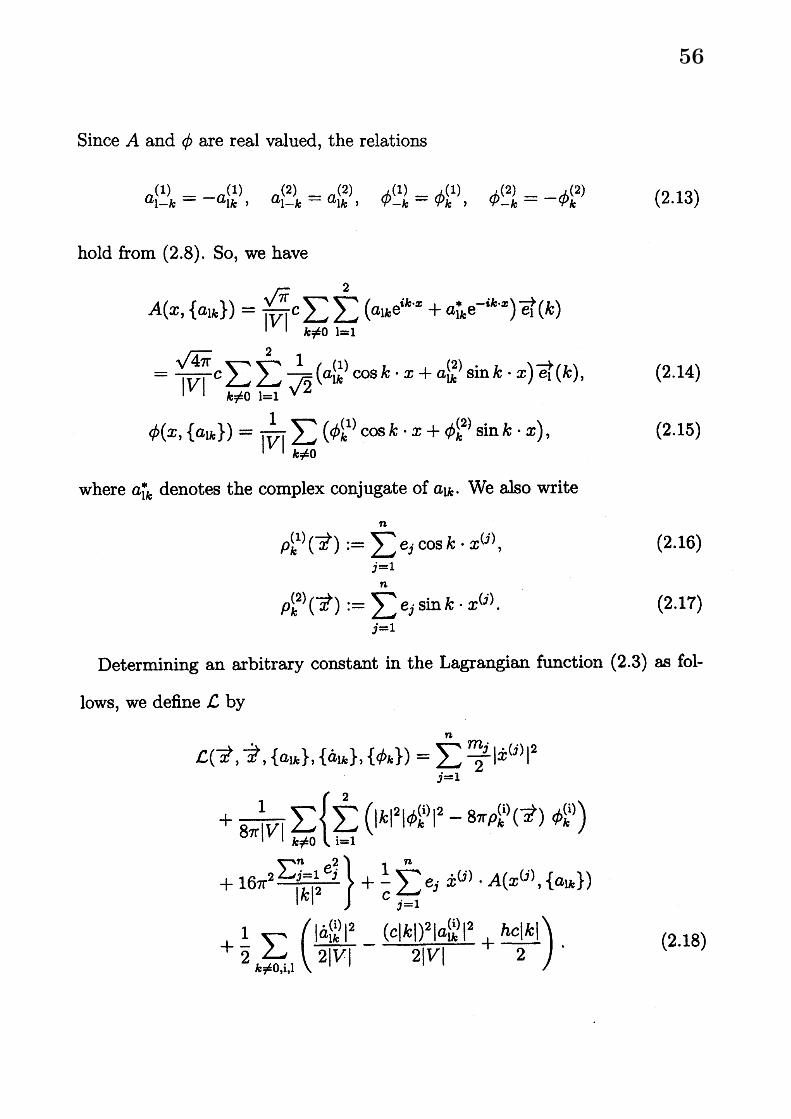
Since $A$ and $\phi$ are real valued, the relations

$a_{1-k}^{(1)}=-a_{1k}^{(1)}$ , $a_{1-k}^{(2)}=a_{1k}^{(2)}$ , $\phi_{-k}^{(1)}=\phi_{k}^{(1)}$ , $\phi_{-k}^{(2)}=-\phi_{k}^{(2)}$ (2.13)

hold from (2.8). So, we have

$A(x, \{a_{1k}\})=\frac{\sqrt{\pi}}{|V|}c\sum_{k\neq 0}\sum_{1=1}^{2}(a_{1k}e^{ik\cdot x}+a_{1k}^{*}e^{-ik\cdot x})e_{1}arrow(k)$

$= \frac{\sqrt{4\pi}}{|V|}c\sum_{k\neq 0}\sum_{1=1}^{2}\frac{1}{\sqrt{2}}$ ($a_{1k}^{(1)}$ cos $k\cdot x+a_{1k}^{(2)}$ sin $k\cdot x$) $e_{1}arrow(k)$ , (2.14)

$\phi(x, \{a_{1k}\})=\frac{1}{|V|}\sum_{k\neq 0}$ ( $\phi_{k}^{(1)}$ cos $k\cdot x+\phi_{k}^{(2)}$ sin $k\cdot x$), (2.15)

where $a_{1k}^{*}$ denotes the complex conjugate of $a_{1k}$ . We also write

$\rho_{k}^{(1)}(7)$ $:= \sum_{j=1}^{n}e_{j}$ cos $k\cdot x^{(j)}$ , (2.16)

$\rho_{k}^{(2)}(\ovalbox{\tt\small REJECT})$

$:= \sum_{j=1}^{n}e_{j}$ sin $k\cdot x^{(j)}$ . (2.17)

Determining an arbitrary constant in the Lagrangian function (2.3) as fol-

lows, we define $\mathcal{L}$ by

$\mathcal{L}(-\partial,\dot{7}, \{a_{1k}\}, \{\dot{a}_{1k}\}, \{\phi_{k}\})=\sum_{j=1}^{n}\frac{m_{j}}{2}|\dot{x}^{(j)}|^{2}$

$+ \frac{1}{8\pi|V|}\sum_{k\neq 0}\{\sum_{i=1}^{2}(|k|^{2}|\phi_{k}^{(i)}|^{2}-8\pi p_{k}^{(i)}(\Rightarrow)\phi_{k}^{(i)})$

$+16 \pi^{2}\frac{\sum_{j--1}^{n}e_{j}^{2}}{|k|^{2}}\}+\frac{1}{c}\sum_{j=1}^{n}e_{j}\dot{x}^{(j)}\cdot A(x^{C)}, \{a_{1k}\})$

$+ \frac{1}{2}\sum_{k\neq 0,i1},(\frac{|\dot{a}_{1k}^{(i)}.|^{2}}{2|V|}-\frac{(c|k|)^{2}|a_{1k}^{(i)}|^{2}}{2|V|}+\frac{hc|k|}{2}I\cdot$ (2.18)

56

Taking account of the constraint condition

$|k|^{2}\phi_{k}^{(i)}=4\pi\rho_{k}^{(i)}$ $(i=1,2, k\neq 0)$ , (2.19)

roughly $\nabla\cdot E=4\pi p$ (cf. (9-17) in [5] and (7.38) in [15]), then we have

$\mathcal{L}_{c}(?, ?, \{a_{1k}\}, \{\dot{a}_{1k}\})=\sum_{j=1}^{n}\frac{m_{j}}{2}|\dot{x}^{(j)}|^{2}$

$- \frac{2\pi}{|V|}\sum_{j\neq l}^{n}\sum_{k\neq 0}\frac{e_{j}e_{l}\cos k\cdot(x^{0)}-x^{(l)})}{|k|^{2}}$

$+ \frac{1}{c}\sum_{j=1}^{n}e_{j}\dot{x}^{(j)}\cdot A(x^{(j)}, \{a_{1k}\})$

$+ \frac{1}{2}\sum_{k\neq 0,i1},(\frac{|\dot{a}_{1k}^{(i)}|^{2}}{2|V|}-\frac{(c|k|)^{2}|a_{1k}^{(i)}|^{2}}{2|V|}+\frac{hc|k|}{2})$ . (2.20)

3 Results under the constraint condition.

We arbitrarily cut off the terms of large wave numbers $k$ in (2.20). That

is, let $M_{j}(j=1,2,3)$ be arbitrary positive integers such that $M_{2}\leq M_{3}$ . We

consider

$\Lambda_{j}$ $:= \{k=(\frac{2\pi}{L_{1}}s_{1},$ $\frac{2\pi}{L_{2}}s_{2},$ $\frac{2\pi}{L_{3}}s_{3})$ ; $s_{1}^{2}+s_{2}^{2}+s_{3}^{2}\neq 0$ ,

$|s_{1}|,$ $|s_{2}|,$ $|s_{3}|\leq M_{j}\}$ (3.1)

and write

$\Lambda_{j}=:\Lambda_{j}’\cup-\Lambda_{j}’,$ $\Lambda_{j}’\cap-\Lambda_{j}’=empty$ set, $\Lambda_{2}’\subseteq\Lambda_{3}’$ . (3.2)

Let $N_{j}$ denotes the number of elements of the set $\Lambda_{j}’$ . It follows from (2.13)

that independent variables are $a_{\Lambda_{j}’}:=\{a_{1k}^{(i)}\}_{k\in\Lambda’,i,1}\in R^{4N_{j}}$ (cf. p. 154 in [14]).

57

We consider

$\tilde{\mathcal{L}}_{c}(?, 7, \{a_{1k}\}, \{\dot{a}_{1k}\})$$:= \sum_{j=1}^{n}\frac{m_{j}}{2}|\dot{x}^{(j)}|^{2}$

$- \frac{2\pi}{|V|}\sum_{j\neq l}^{n}\sum_{k\in\Lambda_{1}}\frac{e_{j}e_{l}\cos k\cdot(x^{C)}-x^{(l)})}{|k|^{2}}$

$+ \frac{1}{c}\sum_{j=1}^{n}e_{j}\dot{x}^{(j)}\cdot\tilde{A}(x^{(j)}, \{a_{1k}\})$

$+ \frac{1}{2}\sum_{k\in\Lambda_{\theta},i,1}(\frac{|\dot{a}_{1k}^{(i)}|^{2}}{2|V|}-\frac{(c|k|)^{2}|a_{1k}^{(i)}|^{2}}{2|V|}+\frac{hc|k|}{2})$ (3.3)

in place of $C_{c}$ , where $A$ given by (2.14) is replaced with

$\tilde{A}(x, \{a_{1k}\})=\frac{\sqrt{4\pi}}{|V|}cg(x)\sum_{k\in\Lambda_{2}}\sum_{1=1}^{2}(\psi(a_{1k}^{(1)}/\sqrt{2})$ cos $k\cdot x$

$+\psi(a_{1k}^{(2)}/\sqrt{2})$ sin $k\cdot x)e_{1}arrow(k)$ . (3.4)

We suppose $\psi(-\theta)=-\psi(\theta)(\theta\in R)$ . We note that if $g=1$ and $\psi(\theta)=\theta$ ,

then $\tilde{A}=A$ .

For the sake of simplicity we suppose $\Lambda’$ $:=\Lambda_{1}’=\Lambda_{2}’=\Lambda_{3}’$ . Let

$\Delta$ : $0=\tau_{0}<\tau_{1}<\ldots<\tau_{\nu}=T$, $|\Delta|$$:= \max_{1\leq l\leq\nu}(\tau_{l}-\tau_{l-1})$ .

Let $\Leftrightarrow\in R^{3n}$ and $a_{\Lambda’}\in R^{4N}(N:=N_{1})$ be fixed. We take arbitrarily

$7^{(0)},$ $\ldots?(\nu-1)\in R3n$

and$a_{\Lambda}^{(0)},$

$\ldots,$$a_{\Lambda}^{(\nu-1)}\in R^{4N}$ .

Then, we write the broken line paths on $[0,T]$ connecting $\Rightarrow(l)$ at $\theta=\tau_{l}(l=$

$0,1,$ $\ldots$ , $\nu,$$i^{(\nu)}=-\theta$ ) in order as $7_{\Delta}(\theta)\in R^{3n}$ . In the same way we define

58

the broken line paths $a_{\Lambda’\Delta}(\theta)\in R^{4N}$ on $[0, T]$ for $a_{\Lambda}^{(0)},$

$\ldots,$$a_{\Lambda}^{(\nu-1)}$ and $a_{\Lambda’}$ . We

define $a_{\Lambda\Delta}(\theta)\in R^{8N}$ by means of (2.13). We write the classical action

$\tilde{S}_{c}(T, 0;7_{\Delta}, a_{\Lambda\Delta})=\int_{0}^{T}\tilde{\mathcal{L}}_{c}(7_{\Delta}(\theta), 7_{\Delta}(\theta)$,

$a_{\Lambda\Delta}(\theta),\dot{a}_{\Lambda\Delta}(\theta))d\theta$ . (3.5)

THEOREM 3.1. We assume for $g(x)$ and $\psi(\theta)$ in (3.4) that for any $l=$

$1,2,$ $\ldots$ and any multi-index $\alpha$ there enist constants $\delta_{l}>0$ and $\delta_{\alpha}>0$ satisfying

$|\partial_{\theta}^{l}\psi(\theta)|\leq C_{l}(1+|\theta|)^{-(1+\delta_{l})},$ $\theta\in R$

and

$|\partial_{x}^{\alpha}g(x)|\leq C_{\alpha}(1+|x|)^{-(1+\delta_{\alpha})},$ $x\in R^{3}$ ,

respectively. Let $f(*, a_{\Lambda’})\in L^{2}(R^{3n+4N})$ . We write

$\cross Os-\int\int(\exp ih^{-1}\tilde{S}_{c}(T, 0;7_{\Delta}, a_{\Lambda\Delta}))f(7_{\Delta}(0)$ ,

$a_{\Lambda’\Delta}(0))d7^{(0)}\cdots d3^{(\nu-1)}da_{\Lambda}^{(0)}\cdots da_{\Lambda}^{(\nu-1)}$ (3.6)

as $(C_{\Delta}(T, 0)f)(7, a_{\Lambda’})$ or $\int\int(\exp ih^{-1}\tilde{S}_{c}(T, 0;7_{\Delta}, a_{\Lambda\Delta}))f(7_{\Delta}(0), a_{\Lambda’\Delta}(0))$

$\cross \mathcal{D}7_{\Delta}Da_{\Lambda’\Delta}$ . Then, as $|\Delta|$ tends to $0$ , the function $(C_{\Delta}(T, 0)f)(7, a_{\Lambda’})$ con-

verges to the so-cdled Feynman path integral $\iint(\exp ih^{-1}\tilde{S}_{c}(T, 0;v_{a_{\Lambda}})f($

$7(0),$ $a_{\Lambda}’(0))\mathcal{D}7\mathcal{D}a_{\Lambda}$’ in $L^{2}(R^{3n+4N})$ . In addition, this limit satisfies the

Schrodinger type equation

$ih \frac{\partial}{\partial t}u(t)=H(t)u(t),$ $u(O)=f$, (3.7)

59

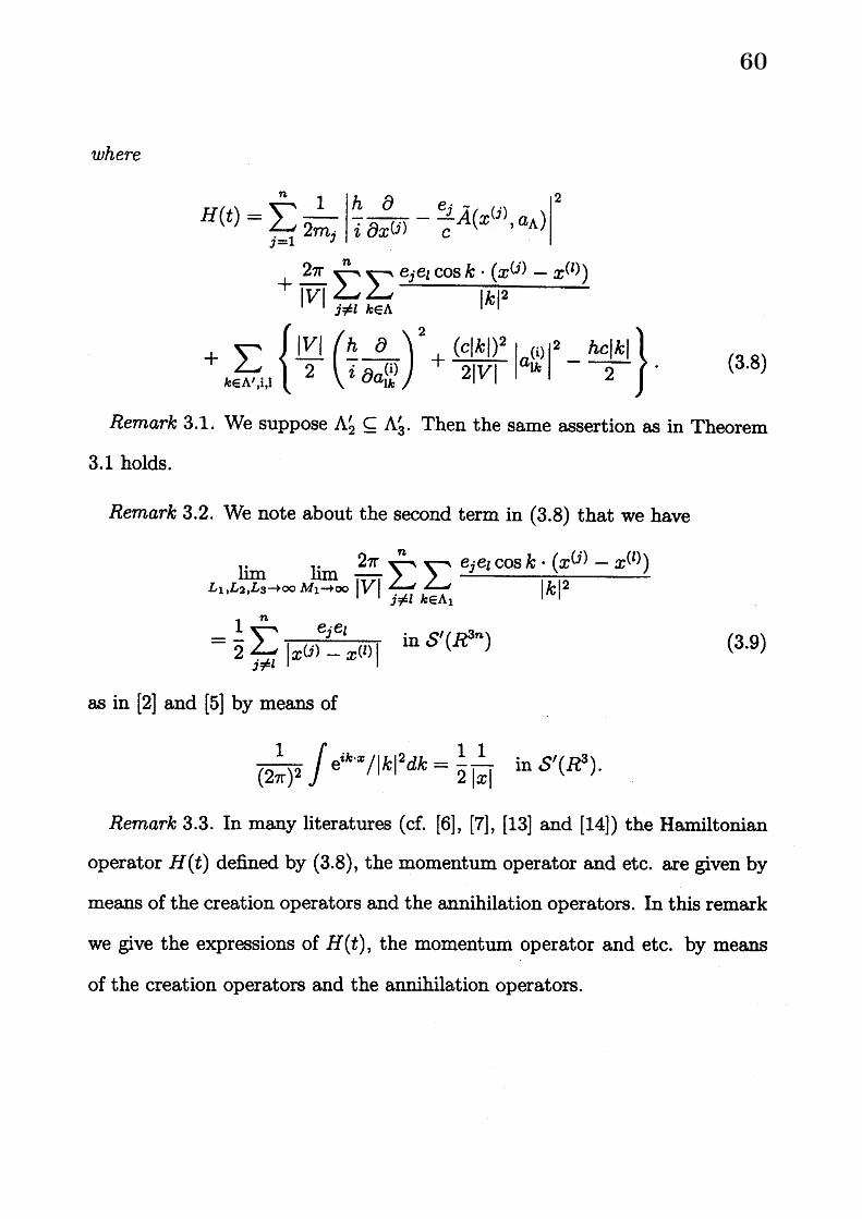
where

(3.8)

$H(t)= \sum_{j=1}^{n}\frac{1}{2m_{j}}|\frac{h}{i}\frac{\partial}{\partial x^{(j)}}-\frac{e_{j}}{c}\tilde{A}(x^{(j)}, a_{\Lambda})|^{2}$

$+ \frac{2\pi}{|V|}\sum_{j\neq l}^{n}\sum_{k\in\Lambda}\frac{e_{j}e_{l}\cos k\cdot(x^{(j)}-x^{(l)})}{|k|^{2}}$

$+ \sum_{k\in\Lambda’,i1},\{\frac{|V|}{2}(\frac{h}{i}\frac{\partial}{\partial a_{1k}^{(i)}})^{2}+\frac{(c|k|)^{2}}{2|V|}|a_{1k}^{(i)}|^{2}-\frac{hc|k|}{2}\}$ .

Remark 3.1. We suppose $\Lambda_{2}’\subseteq\Lambda_{3}’$ . Then the same assertion as in Theorem

3.1 holds.

Remark 3.2. We note about the second term in (3.8) that we have

$\lim_{L_{1},L_{2},L_{S}arrow\infty}\lim_{M_{1}arrow\infty}\frac{2\pi}{|V|}\sum_{j\neq l}^{n}\sum_{k\in\Lambda_{1}}\frac{e_{j}e_{l}\cos k\cdot(x^{(j)}-x^{(l)})}{|k|^{2}}$

$= \frac{1}{2}\sum_{j\neq l}^{n}\frac{e_{j}e_{l}}{|x^{(j)}-x^{(l)}|}$ in $S’(R^{3n})$ (3.9)

as in [2] and [5] by means of

$\frac{1}{(2\pi)^{2}}\int e^{ik\cdot x}/|k|^{2}dk=\frac{1}{2}\frac{1}{|x|}$ in $S’(R^{3})$ .

Remark 3.3. In many literatures (cf. [6], [7], [13] and [14]) the Hamiltonian

operator $H(t)$ defined by (3.8), the momentum operator and etc. are given by

means of the creation operators and the annihilation operators. In this remark

we give the expressions of $H(t)$ , the momentum operator and etc. by means

of the creation operators and the annihilation operators.

60

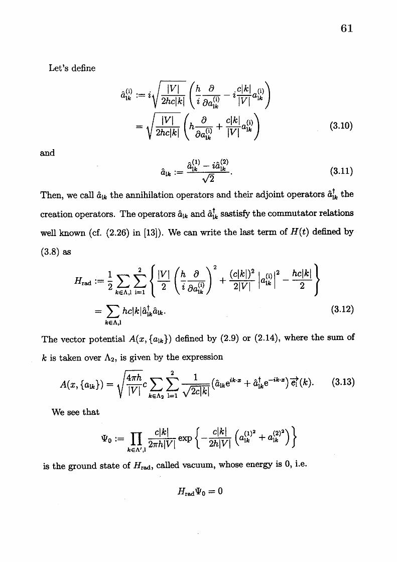
Let’s define

$\hat{a}_{1k}^{(i)}$ $:=i \sqrt{\frac{|V|}{2hc|k|}}(\frac{h}{i}\frac{\partial}{\partial a_{1k}^{(i)}}-\frac{c|k|}{|V|}a_{1k}^{(i))}$

$= \sqrt{\frac{|V|}{2hc|k|}}(h\frac{\partial}{\partial a_{1k}^{(i)}}+\frac{c|k|}{|V|}a_{1k}^{(i))}$ (3.10)

and

$\hat{a}_{1k}:=\frac{\hat{a}_{1k}^{(1)}-i\hat{a}_{1k}^{(2)}}{\sqrt{2}}$ . (3.11)

Then, we call $\hat{a}_{1k}$ the annihilation operators and their adjoint operators $\hat{a}_{1k}^{\dagger}$ the

creation operators. The operators $\hat{a}_{1k}$ and $\hat{a}_{1k}^{1}$ sastisfy the commutator relations

well known (cf. (2.26) in [13]). We can write the last term of $H(t)$ defined by

(3.8) as

$H_{rad}$ $:= \frac{1}{2}\sum_{k\in\Lambda,1}\sum_{i=1}^{2}\{\frac{|V|}{2}(\frac{h}{i}\frac{\partial}{\partial a_{1k}^{(i)}})^{2}+\frac{(c|k|)^{2}}{2|V|}|a_{1k}^{(i)}|^{2}-\frac{hc|k|}{2}\}$

$= \sum_{k\in\Lambda,1}hc|k|\hat{a}_{1k}^{\dagger}\hat{a}_{1k}$. (3.12)

The vector potential $A(x, \{a_{1k}\})$ defined by (2.9) or (2.14), where the sum of

$k$ is taken over $\Lambda_{2}$ , is given by the expression

$A(x, \{a_{1k}\})=\sqrt{\frac{4\pi h}{|V|}}c\sum_{k\in\Lambda_{2}}\sum_{1=1}^{2}\frac{1}{\sqrt{2c|k|}}(\hat{a}_{1k}e^{ik\cdot x}+\hat{a}_{1k}^{\uparrow}e^{-ik\cdot x})e_{1}arrow(k)$ . (3.13)

We see that

$\Psi_{0}$ $:= \prod_{k\in\Lambda’1},\frac{c|k|}{2\pi h|V|}\exp\{-\frac{c|k|}{2h|V|}(a_{1k}^{(1)^{2}}+a_{1k}^{(2)^{2}})\}$

is the ground state of $H_{rad}$ , called vacuum, whose energy is $0$ , i.e.

$H_{rad}\Psi_{0}=0$

61

and satisfies

$\hat{a}_{1k}^{\uparrow}\Psi_{0=}\sqrt{\frac{2c|k|}{h|V|}}a_{1k}^{*}\Psi_{0},\hat{a}_{1k}\Psi_{0}=0$ (3.14)

(cf. Problem 9-8 in [5]). The function $\Psi_{n’1k}$ $:=(\hat{a}_{1k}^{1})^{n’}\Psi_{0}(n’=1,2, \ldots)$ , which

can be written in the concrete from (3.10) and (3.11), called $n’$ photons with

the momentum $hk$ and the polarization state 1 (cf. [13]), satisfies

$( \sum_{k\in\Lambda,1}\hat{a}_{\iota k}^{\dagger}\hat{a}_{1k})\Psi_{n’1’k’}=n’\Psi_{n’1’k’}$ , (3.15)

$( \sum_{k\in\Lambda}hk\hat{a}_{1k}^{\dagger}\hat{a}_{1k})\Psi_{n’1’k’}=n’(hk’)\Psi_{n’1’k’}$ (3.16)

and

$H_{rad}\Psi_{n’1’k’}=n’(hc|k’|)\Psi_{n’1’k’}$ (3.17)

from (3.14) and the commutation relations. We note that we assumed $\int Adx=$

$0$ , i.e. $a_{10}^{(i)}=0(i, 1=1,2)$ in (2.6). The operators defined by the left hand

side of (3.15) and (3.16) are called the number operator and the momentum

operator, respectively (cf. [13]).

Remark 3.4. In many literaturs (cf. [5], [13] and [14]) an arbitrary constant

in the Lagrangian function (2.3) is determined to be $0$ . Consequently, the

term $(1/2) \sum_{j=1}^{n}e_{j}^{2}/|x^{(j)}-x^{(j)}|$ appears in (3.9) and the ground state energy

of $H_{rad}$ is $\sum_{k\in\Lambda}hc|k|/2$ , which tends to infinity when $M_{3}$ tends to infinity.

In the present paper we determined an arbitrary constant in (2.3) by (2.18).

Consequently, we could see that the term $(1/2) \sum_{j=1}^{n}e_{j}^{2}/|x^{(j)}-x^{(j)}|$ disappears

in (3.9) and that the ground state energy of $H_{rad}$ becomes $0$ .

62

Remark 3.5. We consider the external electromagnetic field $E_{ex}(t, x)=(E_{ex1}$ ,

$E_{ex2},$ $E_{ex3}$ ) $\in R^{3}$ and $B_{ex}(t, x)=(B_{ex1}, B_{ex2}, B_{ex3})\in R^{3}$ . We assume as in Ichi-

nose [8] that for any $\alpha\neq 0$ there exist constants $C_{\alpha}$ and $\delta_{\alpha}>0$ satisfying

$|\partial_{x}^{\alpha}E_{exj}(t, x)|\leq C_{\alpha},$ $|\alpha|\geq 1,$ $|\partial_{x}^{\alpha}B_{exj}(t,x)|\leq C_{\alpha}(1+|x|)^{-(1+\delta_{a})}$

$(j=1,2,3)$ in $[0,T]\cross R^{n}$ . Let $\phi_{ex}(t, x)\in R$ and $A_{ex}(t, x)\in R^{3}$ be the electro-

magnetic potential to $E_{ex}$ and $B_{ex}$ . We replace $\tilde{A}(x, \{a_{1k}\})$ in (3.3) and (3.8)

with $\tilde{A}(x, \{a_{1k}\})+\sum_{j=1}^{n}A_{ex}(t,x^{(j)})$ . Moreover we $add-\sum_{j=1}^{n}e_{j}\phi_{ex}(t,x^{(j)})$ to

(3.3) and $\sum_{j=1}^{n}e_{j}\phi_{ex}(t,x^{(j)})$ to (3.8), respectively. Then, the same assertion as

in Theorem 3.1 holds.

The outline of the proof of Theorem 3.1. Let $||f\Vert$ denote the $L^{2}$ norm for

a function $f(7, a_{\Lambda’})$ on $R^{3n+4N}$ . For $a=1,2,$ $\ldots$ we consider the weighted

Sobolev spaces

$B^{a}$ $:=\{f(?, a_{\Lambda’})\in L^{2}(R^{3n+4N});\Vert f||_{B^{a}}$ $:=\Vert f\Vert+$

$\sum_{|\alpha|=a}(||x^{\alpha}f\Vert+\Vert(h\partial_{x})^{\alpha}f\Vert)<\infty\},$

$x:=(R, a_{\Lambda’})$ . (3.18)

We set $B^{0}=L^{2}$ . Then, we can prove:

(1) There exist constants $p^{*}>0$ and $K_{a}\geq 0(a=0,1,2, \ldots)$ such that for

$0\leq t\leq T$ we have

$\Vert C_{\Delta}(t, 0)f\Vert_{B^{a}}\leq e^{K_{a}T}\Vert f||_{B^{a}},$ $0\leq|\Delta|\leq\rho^{*}$ , (3.19)

where $C_{\Delta}(t, 0)f$ was defined by (3.6).

(2) There exists a constant $M\geq 2$ such that for $\leq t,t’\leq T$ and $a=0,1,2,$ $\ldots$

63

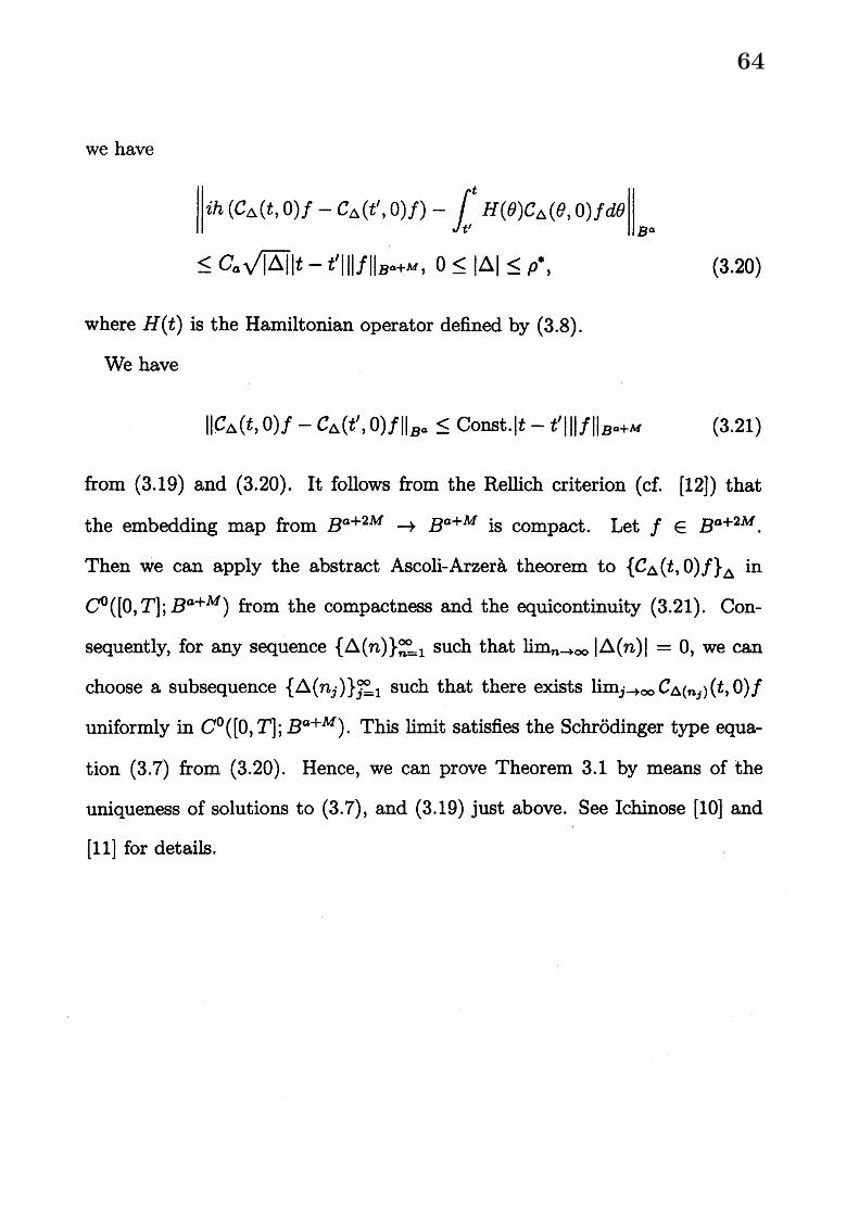
we have

$\Vert ih(C_{\Delta}(t, O)f-C_{\Delta}(t’, O)f)-\int_{t}^{t}H(\theta)C_{\Delta}(\theta, 0)fd\theta\Vert_{B^{a}}$

$\leq C_{a}\sqrt{|\Delta|}|t-t’|\Vert f\Vert_{B^{a+M}},$ $0\leq|\Delta|\leq\rho^{*}$ , (3.20)

where $H(t)$ is the Hamiltonian operator defined by (3.8).

We have

$||C_{\Delta}(t, O)f-C_{\Delta}(t’, 0)f\Vert_{B^{a}}\leq Const.|t-t’|\Vert f||_{B^{a+M}}$ (3.21)

Rom (3.19) and (3.20). It follows from the Rellich criterion (cf. [12]) that

the embedding map from $B^{a+2M}arrow B^{a+M}$ is compact. Let $f\in B^{a+2M}$ .

Then we can apply the abstract Ascoli-Arzer\‘a theorem to $\{C_{\Delta}(t, O)f\}_{\Delta}$ in

$C^{0}([0,T];B^{a+M})$ from the compactness and the equicontinuity (3.21). Con-

sequently, for any sequence $\{\Delta(n)\}_{n=1}^{\infty}$ such that $\lim_{narrow\infty}|\Delta(n)|=0$ , we can

choose a subsequence $\{\Delta(n_{j})\}_{j=1}^{\infty}$ such that there exists $\lim_{jarrow\infty}C_{\Delta(n_{j})}(t, O)f$

uniformly in $C^{0}([0,T];B^{a+M})$ . This limit satisfies the Schr\"odinger type equa-

tion (3.7) $hom(3.20)$ . Hence, we can prove Theorem 3.1 by means of the

uniqueness of solutions to (3.7), and (3.19) just above. See Ichinose [10] and

[11] for details.

64

4Results without the constraint condition.

In place of $\mathcal{L}$ expressed by (2.18) we consider

$\tilde{C}(?,\dot{i}, \{a_{1k}\}, \{\dot{a}_{1k}\}, \{\phi_{k}\}):=\sum_{j=1}^{n}\frac{m_{j}}{2}|\dot{x}^{(j)}|^{2}$

$+ \frac{1}{8\pi|V|}\sum_{k\in\Lambda_{1}}\{\sum_{i=1}^{2}(|k|^{2}|\phi_{k}^{(i)}|^{2}-8\pi\rho_{k}^{(i)}(7)\phi_{k}^{(i)})$

$+16 \pi^{2}\frac{\sum_{j--1}^{n}e_{j}^{2}}{|k|^{2}}\}+\frac{1}{c}\sum_{j=1}^{n}e_{j}\dot{x}^{(i)}\cdot\tilde{A}(x^{(i)}, \{a_{1k}\})$

$+ \frac{1}{2}\sum_{k\in\Lambda_{3},i,1}(\frac{|\dot{a}_{1k}^{(i)}|^{2}}{2|V|}-\frac{(c|k|)^{2}|a_{1k}^{(i)}|^{2}}{2|V|}+\frac{hc|k|}{2})$ (4.1)

by means of (3.4) as in $C_{c}$ , where we suppose $\Lambda_{2}\subseteq\Lambda_{3}$ . For the sake of

simplicity we again suppose $\Lambda’$ $:=\Lambda_{1}’=\Lambda_{2}’=\Lambda_{3}’$ as in Theorem 3.1.

$Let7_{\Delta}(\theta)\in R^{3n},$ $a_{\Lambda’\Delta}(\theta)\in R^{4N}$ and $a_{\Lambda\Delta}(\theta)\in R^{8N}$ be the broken line paths

defined before. $Letarrow\xi_{k}$$:=\{\xi_{k}^{(i)}\}_{i=1,2}\in R^{2}$ for $k\in\Lambda’$ . Take $arrow\xi_{k}^{(0)},$ $arrow\xi_{k}^{(1)},$

$\ldots$ and

$arrow\xi_{k}^{(\nu-1)}$ in $R^{2}$ arbitrarily. Let $p_{k}:=(p_{k}^{(1)}, p_{k}^{(2)})$ from (2.16) and (2.17). Then,

we define the path

$\phi_{k\Delta}(\theta)$$:= arrow\xi_{k}^{(l)}+\frac{4\pi\rho_{k}(7_{\Delta}(\theta))}{|k|^{2}}\in R^{2},$ $\tau_{l-1}<\theta\leq\tau_{l}$ (4.2)

$(l=1,2, \ldots, \nu)$ , where $\phi_{k\Delta}(0);=\lim_{\thetaarrow 0+0}\phi_{k\Delta}(\theta)$ . We set $\phi_{\Lambda’\Delta}(\theta):=\{\phi_{k\Delta}(\theta)\}_{k\in\Lambda’}$

$\in R^{2N}$ . We define $\phi_{\Lambda\Delta}(\theta)\in R^{4N}$ by means of (2.13). Let $\tilde{S}(T, 0;7_{\Delta}, a_{\Lambda\Delta}, \phi_{\Lambda\Delta})$

be the classical action for $\tilde{\mathcal{L}}(7, 7, \{a_{1k}\}, \{\dot{a}_{1k}\}, \{\phi_{k}\})$ .

THEOREM 4.1. Let $f(\ovalbox{\tt\small REJECT}, a_{\Lambda’})\in B^{a}(R^{3n+4N})(a=0,1, \ldots)$ . Then as a

65

function in $B^{a}(R^{3n+4N})$ we see that

$( \prod_{j=1}^{n}\prod_{l=1}^{\nu}\sqrt{\frac{m_{j}}{2\pi ih(\tau_{l}-\tau_{l-1})}}^{3})\prod_{l=1}^{\nu}\{\prod_{k\in\Lambda’}(-\frac{i|k|^{2}(\tau_{l}-\tau_{l-1})}{4h\pi^{2}|V|})$

$4N$

$\cross\sqrt{\frac{1}{2|V|\pi ih(\tau_{l}-\tau_{l-1})}}$ $\}os-\int\cdots\int(\exp ih^{-1}\tilde{S}(T,$ $0$ ;

$7_{\Delta},$$a_{\Lambda\Delta},$

$\phi_{\Lambda\Delta}$ ) $)f(7_{\Delta}(0), a_{\Lambda’\Delta}(0))d7^{(0)}\cdots d^{-}i^{(\nu-1)}$

$\cross da_{\Lambda}^{(0)}\cdots da_{\Lambda}^{(\nu-1)}\prod_{k\in\Lambda’}d\xi_{k}^{(0)}d\xi_{k}^{(1)}\cdots d^{arrow}\xi_{k}^{(\nu-1)}arrowarrow$ (4.3)

is equal to

$\int\int(\exp ih^{-1}\tilde{S}_{c}(T, 0;7_{\Delta}, a_{\Lambda\Delta}))$

$\cross f(7_{\Delta}(0), a_{\Lambda’\Delta}(0))\mathcal{D}7_{\Delta}\mathcal{D}a_{\Lambda’\Delta}$

defined by (3.6) in Theorem 3.1. So it follows from Theorem 3.1 that as $|\Delta|arrow$

$0$ , then (4.3) converges to the Feynman path integral

$\int\int\int(\exp ih^{-1}\tilde{S}(T, 0;7, a_{\Lambda}, \phi_{\Lambda}))f(7(0), a_{\Lambda’}(0))\mathcal{D}7\mathcal{D}a_{\Lambda’}\mathcal{D}\phi_{\Lambda’}$ , (4.4)

which satisfies the Schrodinger type equation (3.7). This expression (4.4) is

given in \S 9-8 in $Feynman- Hibbs/5J_{2}$ though a concrete definition is not given

there.

Remark 4.1. As was noted in the introduction, the constraint condition

(2.19) isn’t needed in Theorem 4.1 above.

Remark 4.2. We get the similar assertions for (4.3) as in Theorem 4.1 under

the assumptions of Remark 3.1 and Remark 3.5, respectively.

66

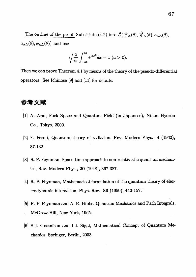
The outline of the proof. Substitute (4.2) into $\tilde{\mathcal{L}}(7_{\Delta}(\theta), 7_{\Delta}(\theta),$ $a_{\Lambda\Delta}(\theta)$ ,

$\dot{a}_{\Lambda\Delta}(\theta),$ $\phi_{\Lambda\Delta}(\theta))$ and use

$\sqrt{\frac{a}{i\pi}}\int_{-\infty}^{\infty}e^{iax^{2}}dx=1(a>0)$ .

Then we can prove Theorem 4.1 by means of the theory of the pseudo-differential

operators. See Ichinose [9] and [11] for details.

参考文献

[1] A. Arai, Fock Spaoe and Quantum Field (in Japanese), Nihon Hyoron

Co., Tokyo, 2000.

[2] E. Fermi, Quantum theory of radiation, Rev. Modern Phys., 4 (1932),

87-132.

[3] R. P. Feynman, Space-time approach to non-relativistic quantum mechan-

ics, Rev. Modem Phys., 20 (1948), 367-387.

[4] R. P. Feynman, Mathematical formulation of the quantum theory of elec-

trodynamic interaction, Phys. Rev., 80 (1950), 440-157.

[5] R. P. Feynman and A. R. Hibbs, Quantum Mechanics and Path Integrals,

$McGraw$-Hill, New York, 1965.

[6] S.J. Gustafson and I.J. Sigal, Mathematical Concept of Quantum Me-

chanics, Springer, Berlin, 2003.

67

[7] F. Hiroshima, Functional integral representation of a model in quantum

electrodynamics, Rev. Math. Phys., 9 (1997), 489-530.

[8] W. Ichinose, On convergence of the Feynman path integral formulated

through broken line paths, Rev. Math. Phys., 11 (1999), 1001-1025.

[9] W. Ichinose, The phase space Feynman path integral with gauge invari-

ance and its convergence, Rev. Math. Phys., 12 (2000), 1451-1463.

[10] W. Ichinose, Convergence of the Feynman path integral in the weighted

Sobolev spaces and the representation of correlation functions, J. Math.

Soc. Japan, 55 (2003), 957-983.

[11] W. Ichinose, Some mathematical remarks on the Feynman path integral

for the quantum electrodynamics, to appear.

[12] M. Reed and B. Simon, Methods of Modem Mathematical Physics IV:

Analysis of Operators, Academic Press, New York, 1978.

[13] J.J. Sakurai, Advanced Quantum Mechanics, Addison-Wesley, Mas-

sachusetts, 1967.

[14] H. Spohn, Dynamics of Charged Particles and Their Radiation Field,

Cambridge University Press, Cambridge, 2004.

[15] M.S. Swanson, Path Integrals and Quantum Process, Academic Press,

Boston, 1992.

68