A mathematical model of a diesel engine for simulation ... · PDF filesimulation of the engine control ... mass in the main parts of the engine. In order to achieve high speed

Global Journal of Pure and Applied Mathematics.

ISSN 0973-1768 Volume 12, Number 1 (2016), pp. 213-228

© Research India Publications

http://www.ripublication.com

A mathematical model of a diesel engine for

simulation modelling of the control system

model for the locomotive diesel engine. The obtained results of HiL-

simulation of the engine control system with the help of the developed

mathematical model confirm the applicability of the proposed method. The

presented results were obtained during research on the development of control

systems and adaptation of sensors and actuators of fuel equipment with

perspective technical parameters with the financial support of the Ministry of

Education and Science of the Russian Federation in the form of subsidies from

the federal budget (code of the lot 2015-14-579-0054).

Keywords: turbocharged diesel engine, mathematical model, functional

dependencies, hardware-in-loop simulation.

Aleksandr Gavriilovich Kuznetsov

“TransSensor” 125480, Russian Federation, Moscow, st. Geroev-Panfilovtsev, 24

Sergey Viktorovich Kharitonov


Dmitriy Sergeevich Vornychev


Abstract

A method for obtaining a mathematical model of an engine is proposed. The

obtained model’s intended use is in the hardware-in-the-loop (HiL) real-time

simulation modelling of the engine control system. The dynamic

characteristics of the turbocharged diesel engine are described by differential

equations of dynamic balance of the flows of mechanical energy and the gas

mass in the main parts of the engine. In order to achieve high speed of

calculations, the parameters requiring a long time for their calculation and the

characteristics that represent the difference between the real and theoretical

engine working cycles are predefined as some relatively simple functional

dependencies. An example is considered of constructing a mathematical

214 Aleksandr Gavriilovich Kuznetsov et al

Introduction In connection with the need to accelerate the process of designing and adjusting the

engines and their control systems, there arose a problem of developing HiL simulation

methods and introducing them into practice. HiL simulation allows producing and

debugging microelectronic devices of engine control system for the real engine

working modes in parallel with the engine creation. Also, HiL simulation saves

money spent on engine tests. In HiL simulation, the real hardware microelectronic

devices are connected to digital implementation of the mathematical model of the

studied engine which allows adjusting the software and control algorithms of the

future power plant control system.

To implement HiL simulation, it is necessary to develop a set of software and

hardware means combined in a single booth. The hardware part of the booth mainly

comprises an electronic control unit (ECU) with a microprocessor at its core. If

needed, the hardware part can be supplemented by actuators, sensors and other

devices of the control system. The information exchange between controller and

digital implementation of the mathematical model is performed by a special interface

device which imitates the engine and some other analyzed parts of the power plant. In

the interface device, the digital codes from the model are transformed into analog

signals corresponding to real signals from physical sensors. These signals are

transmitted to the control unit’s inputs. On the other hand, the interface device also

transforms the electric signals from the control unit into digital codes corresponding

to actuators’ positions and other parameters which affect the model. In the HiL

simulation booth, the ECU interacts with the digital model as if it were the real

engine.

A digital computer model for HiL simulation must meet some specific requirements.

The algorithms of control systems, characteristics and engine operating modes are

determined by the type of power plant in which the studied engine is used as a power

source. That is why a digital implementation of the mathematical model for HiL

simulation must cover not only the engine but also the main parts of the power plant.

For example, a computer model of the vehicle power plant should contain equations

which describe transmission and vehicle as a whole. The mathematical model should

include all kinds of the engine operating modes, both static and dynamic.

The main requirement imposed on such models is the real-time character of the

information exchange between the model and the control unit, appropriate for the

cycle run time of ECU software control algorithms. A single tact of ECU

microcontroller software cycle commonly falls in a range from few to fractions of

milliseconds. Between two consecutive acts of information interchange, all variations

must be performed, the values of the parameters of the power plant and engine

working process in the model must be actualized and the signals from sensors and to

actuators must be generated.

Thereby, a digital implementation of a mathematical model for HiL simulation must

satisfy contradictory requirements: on one hand, it should imitate real dynamic

processes with a sufficient accuracy, on the other hand, it should perform quick

calculations of this processes enough to exchange the data between the model and

ECU in real time. The experience of creating detailed engine models shows that the

A mathematical model of a diesel engine for simulation modelling 215

calculations of operating mode parameters in such models are significantly slower

than the real time scale [1,2,3,4,5]. In this connection, a problem has appeared of

creating “fast” dynamic computer models for performing the HiL simulation. These

models should imitate the engine and the main parts of the power plant with reliable

calculations of working process parameters at high-speed timing (about fractions of

milliseconds).

Method of constructing a mathematical model of an engine In this paper, a method is proposed to solve the formulated problem as applied to a

diesel engine.

This goal is reached by combining the relations from the theory of turbocharged

engine working process and the empirical data in the constructed model.

The problem is to find such compromise mixture of theoretical and empirical parts

that will perform the calculations of dynamic processes with sufficient accuracy and

speed.

In this approach, a number of physical processes in the engine are replaced by

mathematical dependencies between the working process parameters obtained from

the analysis of preliminary experimental or numerical studies.

The argument in favor of this approach is that in the detailed specification of the

engine working process one should use the empirical data, but in the form of

coefficients characterizing the difference between real and theoretical values in the

fuel combustion processes and heat transfer equations. One should also use the values

of internal energy loses in the engine.

It should be noted that the “half-empirical” approaches are successfully used in such

research areas as the theory of regulation, statistics and neural network studies.

In the functional diagram (Fig. 1), a turbocharged diesel engine is represented as a

combination of the following elements:

Figure 1: Functional diagram of a turbocharged diesel engine

the engine itself – cylinders (CY), fuel equipment (FE), turbocharger (TC), the intake

manifold (IM) and the exhaust manifold (EM). In the diagram, the arrows represent

external effects and the interaction of the working process parameters.

Interaction between the parts of a diesel engine is realized mainly through the

following parameters of the working process:

angular velocity of the diesel engine’s shaft 𝜔𝑑;

angular velocity of the turbocharger rotor 𝜔𝑡;

fuel cyclic quantity 𝑔𝑐;


air pressure in the intake manifold 𝑝𝑐;

air pressure in the exhaust manifold 𝑝𝑔.

Several parameters are considered as describing the external effects:

the position of a pedal or lever which affects the fuel injection quantity ℎ;

the environment temperature 𝑇0;

the load torque 𝑀𝑙.

The dynamic characteristics of a turbocharged diesel engine are described by the

equations of dynamic balance of the flows of mechanical energy and gas mass: some

ordinary differential equations for its main elements.

The left-hand side of each equation contains the time derivatives of one of the main

output parameters (Fig. 2): angular speed of the engine shaft 𝜔𝑑, angular speed of the

turbocharger rotor 𝜔𝑡, air pressure in the intake manifold 𝑝𝑐 and in the exhaust

manifold 𝑝𝑔. The right-hand sides of equations contain torques and the gas flow rates.

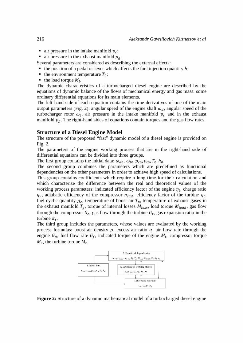
Structure of a Diesel Engine Model The structure of the proposed “fast” dynamic model of a diesel engine is provided on

Fig. 2.

The parameters of the engine working process that are in the right-hand side of

differential equations can be divided into three groups.

The first group contains the initial data: 𝜔𝑑0 , 𝜔𝑡0, 𝑝𝑐0, 𝑝𝑡0 , 𝑇0, ℎ0.

The second group combines the parameters which are predefined as functional

dependencies on the other parameters in order to achieve high speed of calculations.

This group contains coefficients which require a long time for their calculation and

which characterize the difference between the real and theoretical values of the

working process parameters: indicated efficiency factor of the engine 𝜂𝑖, charge ratio

𝜂𝜈 , adiabatic efficiency of the compressor 𝜂𝑐𝑎𝑑, efficiency factor of the turbine 𝜂𝑡,

fuel cyclic quantity 𝑔𝑐, temperature of boost air 𝑇𝑏, temperature of exhaust gases in

the exhaust manifold 𝑇𝑔, torque of internal losses 𝑀𝑙𝑜𝑠𝑠, load torque 𝑀𝑙𝑜𝑎𝑑, gas flow

through the compressor 𝐺𝑐, gas flow through the turbine 𝐺𝑡, gas expansion ratio in the

turbine 𝜋𝑡.

The third group includes the parameters, whose values are evaluated by the working

process formulas: boost air density 𝜌, excess air ratio 𝛼, air flow rate through the

engine 𝐺𝑑, fuel flow rate 𝐺𝑓, indicated torque of the engine 𝑀𝑖, compressor torque

𝑀𝑐, the turbine torque 𝑀𝑡.

Figure 2: Structure of a dynamic mathematical model of a turbocharged diesel engine


The right-hand sides of the differential equations and other necessary parameters of

dynamical model are calculated from the initial data and the predefined functional

dependencies. At each time step of numerical solution of differential equations, the

current values of 𝜔𝑑 , 𝜔𝑡 , 𝑝𝑐 , 𝑝𝑔 are renewed for the further use in the right-hand sides

of equations instead of the corresponding initial data values.

A distinctive feature of our model is the use of the functional dependencies between

the working process parameters (the second group of parameters in Fig. 2) which

reduce the calculation time of the dynamic processes, thus providing a possibility of

application of the model in the real-time HiL simulation.

To obtain the mentioned dependencies, an analysis of the turbocharged diesel engine

working process was performed which resulted in establishing the relations between

the defined parameters and their arguments.

The analysis was mainly based on the literature sources [6,7,8,9,10], which describe

the theory of turbocharged diesel engine and provide the characteristics of certain

engines.

Equations for the Elements of a Turbocharged Diesel Engine The mathematical equations included into the considered “fast” dynamic model of

turbocharged diesel engine are listed below.

A. Cylinders and fuel equipment

The dynamic balance of the mechanical energy of diesel and the energy consumer

(the locomotive tractive motor) is described by the differential equation for the

rotation of shaft, which characterizes the variation over time 𝑡 of the angular velocity

𝜔𝑑 of the diesel generator: 𝑑𝜔𝑑

𝑑𝑡=

1

𝐼𝑑

(𝑀𝑖 − 𝑀𝑙𝑜𝑠𝑠 − 𝑀𝑙𝑜𝑎𝑑),

where 𝐼𝑑 is the diesel generator’s moment of inertia, 𝑀𝑖 is the indicated torque of the

diesel, 𝑀𝑙𝑜𝑠𝑠 is the internal losses torque and 𝑀𝑙𝑜𝑎𝑑 is the load torque.

The main indicator of the fuel combustion effectiveness in diesel engine cylinders is

the indicated effectiveness factor 𝜂𝑖.

The indicated effectiveness is affected by the excess air ratio 𝛼, gas expansion ratio of

combusiton 𝜆, degree of fuel distribution irregularity in the combustion chamber, the

speed mode 𝜔𝑑 and the density of air enering the cylinders 𝜌.

Direct influence of density on the indicated effectiveness factor is insignificant and

acts mainly through the changes in 𝛼 and 𝜆.

The expansion ratio 𝜆 of gases in the combustion process is one of major indicator of

the working cycle dynamics. It is directly affected by the portion of heat released in

the first two periods of combustion, and this portion is determined by the portion of

fuel injected into the combustion chamber during the period of ignition lag.

The influence of the fuel distribution irregularity on 𝜂𝑖 with a chosen method of

mixing is realized through the quantities 𝜔𝑑 and 𝛼.

The conducted analysis of the dependence of the indicated effectiveness on other


parameters of the working process shows that the biggest impact on 𝜂𝑖 is made by air

excess ratio 𝛼 and angular velocity of the engine shaft 𝜔𝑑. Therefore, in the

calculations, the indicated effectiveness factor was set as a function 𝜂𝑖(𝛼, 𝜔𝑑).

The charge ratio 𝜂𝜈 expresses the difference between the amount of air entering the

engine and the amount of air which can fill cylinders with given 𝑝𝑐 and 𝑇𝑐 before

intake valves. The value of 𝜂𝑛𝑢 is significantly influenced by losses in the intake and

exhaust manifolds and by the heat transfer from the warmed cylinder surface to air

charge. With the increase of angular speed of engine shaft, the speed of intake air

charge and exhaust gases also rise. This leads to the growth of losses and reduction of

𝜂𝜈 . The increase of boost pressure 𝑝𝑐 results in the decrease of relative pressure losses

at intake so the charge ratio grows. The influence of charge heating for different

operating modes can be characterized by 𝜔𝑑 and 𝑝𝑐. Thus, the charge ratio can be

specified as a function 𝜂𝜈(𝜔𝑑, 𝑝𝑐).

The model includes an assumption of small impact of the fuel equipment dynamic

properties on the fuel injection process. Therefore, the cyclic fuel quantity can be

specified as an algebraic function of position or opening time of fuel dosing lever ℎ

and angular velocity of engine shaft 𝜔𝑑: 𝑔𝑐(ℎ, 𝜔𝑑).

The value of exhaust gases temperature 𝑇𝑔 depends on many factors, primarily, on the

indicated effectiveness factor 𝜂𝑖, air excess ratio 𝛼, parameters of air entering the

engine 𝑝𝑐 and 𝑇𝑎, speed mode 𝜔𝑑 and the coefficient of total heat losses per cycle. An

increase of air excess ratio leads to a decrease of the average gas temperature in the

expansion and exhaust processes and an increase of the indicated effectiveness factor.

A decrease of gas temperature leads to a decrease of heat transfer in the expansion

process. In its turn, an increase of indicated effectiveness factor leads to a decrease of

temperature of the gases leaving cylinders and, as a consequence, to a decrease of heat

transfer in the exhaust process. The total impact of all factors leads to a noticeable

change of total losses per cycle.

As the engine shaft angular velocity grows, the exhaust gases temperature also grows

because of the change of heat release process in cylinder and reduced heat transfer in

the exhaust process. An increase of the boost air temperature which depends on

combination of 𝑝𝑐 and 𝛼 results in the rise of the amount of heat contributed by air

into the engine cylinders. As a result, the gas temperature and total losses per cycle

are rising. Taking into account possible reduction of the number of working process

parameters influencing the exhaust gas temperature, we used a dependence in the

form 𝑇𝑔(𝜔𝑑, 𝛼, 𝑝𝑘).

The internal losses of mechanical energy in the engine consist of the friction losses

and the energy consumed on combustion gases expelling, new air charge filling, on

fuel, grease and cooling equipment driving [11]. The friction losses get higher with

the growth of the speed operating mode. Also friction rises when air boost increases

because of the increased pressure on moving parts. The energy consumption for the

organization of the gas exchange processes depends on the ratio of the input 𝑝𝑐 and

output 𝑝𝑔 pressures. An analysis of the engine characteristics shows that a connection

exists between the values of 𝑝𝑐 and 𝑝𝑔. Therefore, it is preferable to use a function

𝑀𝑙𝑜𝑠𝑠(𝑛𝑑, 𝑝𝑐) for the losses torque.


Other parameters needed for computation of the right-hand sides of differential

equations are determined by the formulas of the theory of the diesel engine working

process with the use of the functions given above.

Considering the equation of state for the intake air as an ideal gas, we get

𝜌 = 𝑝𝑐 (𝑅𝑎𝑇𝑎)⁄ ,

where 𝑅𝑎 = 287𝐽

𝑚𝑜𝑙 ⋅ 𝐾 is the air gas constant.

The air flow rate through the engine

𝐺𝑑 = 𝜌 𝑖𝑉 (𝑛𝑑

120) 𝜂𝜈 ,

where 𝑖 is number of cylinders, 𝑉 is the working volume of cylinder, 𝑛𝑑/120 is the

number of cycles in 1 second, 𝑛𝑑 = 30 𝜔𝑑/𝜋.

The fuel flow rate

𝐺𝑓 = 𝑖 𝑔𝑐𝑛𝑑/120 .

The air excess ratio

𝛼 = 𝐺𝑑/(14,3 𝐺𝑓).

The indicated engine torque

𝑀𝑖 = 𝐻𝑢𝐺𝑓𝜂𝑖/𝜔𝑑 ,

where 𝐻𝑢 = 42500 𝑘𝐽/𝑘𝑔 is the net heating value of the diesel fuel.

B. Turbocharger

The dynamic balance of mechanical energy of turbine and compressor is described by

the equation of turbocharger rotor rotation 𝑑𝜔𝑡

𝑑𝑡=

1

𝐼𝑡

(𝑀𝑡 − 𝑀𝑐) ,

where 𝐼𝑡 is the turbocharger rotor inertia, 𝑀𝑡 is the turbine torque, 𝑀𝑐 is the

compressor torque.

The ratio of work spent on compressor driving considering losses of hydraulic flow

resistance and heat exchange and adiabatic work of compression process is given by

adiabatic effectiveness of compressor 𝜂𝑐𝑎𝑑 .

The parameters that define the compressor operation mode are interconnected. For

some value of rotor angular velocity 𝜔𝑡, the impact of the diesel engine on the

compressor is manifested through the value of air pressure in the intake manifold 𝑝𝑐.

Other parameters of working process such as 𝐺𝑐 and 𝑇𝑐 are determined by the

combination of 𝜔𝑡 and 𝑝𝑐.Therefore, in this model the functions 𝜂𝑐𝑎𝑑(𝜔𝑡 , 𝑝𝑐) and

𝐺𝑐(𝜔𝑡, 𝑝𝑐) are used. The temperature at the compressor output

𝑇𝑐 = 𝑇0 [1 +𝜋𝑐

𝑘−1𝑘

−1

𝜂𝑐𝑎𝑑]

where 𝑘 = 1.4 is the adiabatic index, 𝜋𝑐 = 𝑝𝑐/𝑝0 is the ratio of pressures in

compressor, 𝑝0 is the environment pressure.


Adiabatic work of compressing 1 kg of air in the compressor

𝐿𝑐𝑎𝑑 =𝑘

𝑘−1𝑅𝑎𝑇0 (𝜋𝑐

𝑘−1

𝑘 − 1) .

Actual compression work considering hydraulic resistance and heat exchange

𝐿𝑐 =𝐿𝑐𝑎𝑑

𝜂𝑐𝑎𝑑

The power used for compressor driving (when referring the mechanical losses to

turbine)

𝑁𝑐 = 𝐺𝑐𝐿𝑐𝑎𝑑

𝜂𝑐𝑎𝑑

The torque needed for compressor driving

𝑀𝑐 = 𝑁𝑐/𝜔𝑡

To take into account the effectiveness of transformation of the available heat drop into

mechanical energy, it is necessary to set a turbine effectiveness factor 𝜂𝑡 dependency

on operating mode. The parameters of turbine operating mode are 𝜔𝑡 , 𝜋𝑡 , 𝑇𝑔 , 𝐺𝑡 ,

where 𝜋𝑡 = 𝑝𝑔/𝑝𝑡0 is the ratio of pressure drop between gas entering the turbine 𝑝𝑔

and at the output of turbine 𝑝𝑡0. The data analysis for the V16 diesel engine tests

shows that the ratio of pressure drop in turbine depends mostly on 𝑝𝑔. So in the model

it is set as a function 𝜋𝑡(𝑝𝑔).

Considering the laws of similarity theory, operating mode of turbine can be set as a

combination of pressure drop ratio 𝜋𝑡 and relative angular velocity of rotor 𝜔𝑡𝑟 =

𝜔𝑡/√𝑇𝑔 . These primary parameters are used as arguments for dependencies

𝜂𝑡(𝜔𝑡𝑟 , 𝜋𝑡) and 𝐺𝑡𝑟(𝜔𝑡𝑟 , 𝜋𝑡), where 𝐺𝑡𝑟 = 𝐺𝑡√𝑇𝑔/𝑝𝑔 is the relative gas flow rate

through the turbine.

The obtained characteristics of relative gas flow rate through the turbine of V16 diesel

engine shows that this parameter can be defined as 𝐺𝑡𝑟(𝜔𝑡𝑟).

Other parameters are determined by the formulas of the turbine working process.

Adiabatic work of 1 kg of gas in the turbine

𝐿𝑡𝑎𝑑 =𝑘𝑔

𝑘𝑔 − 1𝑅𝑔𝑇𝑔 (1 − 𝜋𝑡

1−𝑘𝑔

𝑘𝑔 ),

where 𝑘𝑔 = 1.35 is the adiabatic index of the exhaust gases and 𝑅𝑔 = 286 𝐽/(𝑚𝑜𝑙 ⋅

𝐾) is the gas constant of exhaust gases.

Effective part of adiabatic work is transformed into mechanical work of gases

considering losses of flow moving in turbine and friction in turbocharger 𝐿𝑡 = 𝐿𝑡𝑎𝑑𝜂𝑡.

The power of turbine rotor

𝑁𝑡 = 𝐺𝑡𝐿𝑡 .

The torque of turbine rotor

𝑀𝑡 = 𝑁𝑡/𝜔𝑡 .


C. Intake and exhaust manifolds of a diesel engine

Variation of air mass in the intake manifold of diesel 𝑑𝑚𝑎 during the elementary

period of time 𝑑𝑡

𝑑𝑚𝑎 = 𝐺𝑐𝑑𝑡 − 𝐺𝑑𝑑𝑡 From the equation of state of the air as an ideal gas

𝑚𝑎 =𝑉𝑖𝑛𝑝𝑐

𝑅𝑎𝑇𝑎,

where 𝑉𝑖𝑛 is the volume of the intake manifold.

The formula for the air pressure variation in the intake manifold is

𝑑𝑝𝑐

𝑑𝑡=

𝑅𝑎𝑇𝑎

𝑉𝑖𝑛(𝐺𝑐 − 𝐺𝑑)

Variation of gas mass in the intake manifold of diesel engine 𝑑𝑚𝑔 during the

elementary period of time 𝑑𝑡

𝑑𝑚𝑔 = 𝐺𝑑𝑑𝑡 + 𝐺𝑓𝑑𝑡 − 𝐺𝑡𝑑𝑡

Under the applicability assumption of ideal gas state equation to the exhaust gas, we

have

𝑚𝑔 =𝑝𝑔𝑉𝑜𝑢𝑡

𝑅𝑔𝑇𝑔 ,

where 𝑉𝑜𝑢𝑡 is the volume of the outlet manifold.

Equation of gas pressure variation in the exhaust manifold

𝑑𝑝𝑔

𝑑𝑡=

𝑅𝑔𝑇𝑔

𝑉𝑜𝑢𝑡(𝐺𝑑 + 𝐺𝑓 − 𝐺𝑡) .

Functional Dependencies of the Model The most difficult part of obtaining a “fast” dynamic model of the turbocharged diesel

engine is to determine the dependencies between the diesel working process

parameters. Commonly in HiL simulation, the characteristics are given in two ways:

as lookup tables and as functions. Initial data with variations and combinations of

primary working process parameters corresponding to the field of possible dynamic

modes must be used to obtain the characteristics.

Taking into account the low gas inertia of turbocharger, for determination of the

efficiency factors 𝜂𝑐𝑎𝑑 , 𝜂𝑡 and flow rates 𝐺𝑐, 𝐺𝑡 we can use the empirical universal

characteristics of compressor and turbine. The working process of diesel is

determined by the combination of engine and turbocharger parameters. At dynamic

operation modes, equilibrium of the energy and gas flows common to static modes is

disturbed due to mechanical inertia of the cylinder block of engine and turbocharger.

Thereby, the default static speed or load characteristics do not cover all possible

combinations of engine working process parameters.

It is advisable to carry out special experimental studies with independent variations of

primary working process parameters such as fuel quantity and boost air pressure in

order to obtain a detailed description of diesel engine dynamics. Implementation of

these experimental studies is a very complicated problem, because it demands stand-

alone source of boost air instead of default turbocharger [12,13]. Extended static


characteristics of diesel engine can also be obtained by computations with the use of

modern software for engine working process simulation [14,15,16,17].

When using lookup tables, the values of parameters in the second group are given at

the nodes of a grid, the indices of which are variations of primary parameters. The

parameter value at every calculated mode can be obtained by linear interpolation

method. A functional form of working process parameters dependency representation

can be specified as a polynomial with coefficients determined by the least square

method. Selection of the polynomial type should be performed on the basis of the

condition of accord between the described dependencies and the diesel working

process behavior.

The use of polynomial dependencies between the parameters in “fast” dynamic model

allows simulating dynamic modes of transient processes both inside original modes

field (interpolation) and outside of it (extrapolation). The experience of numerical

studies shows that in some models it is expedient to use a combination of

representation of the dependency between the parameters of the engine working

process: both as lookup tables and in a functional form.

Example of Development of A Diesel Engine Model A. Specifics of functional dependencies selection for the model

The proposed method was applied for obtaining computer models of diesel engines

and power plants for different types of vehicles: locomotive and heavy-duty trucks.

The developed models were used in the studies and the formation of initial settings of

control systems.

To illustrate the specifics of the proposed method of mathematical model

construction, we present the results of development of “fast” model of a diesel engine

for the locomotive power plant. The turbocharged diesel engine of the considered

locomotive has 16 cylinders with diameter and stroke of 260 millimeters.

The load characteristics of diesel engine and results of the special studies of transient

modes imitation on single cylinder test stand were used as initial data for the

development of mathematical model of the cylinder block [13].

The results of experimental studies of transient modes imitation confirm the

assumption that the indicated effectiveness factor 𝜂𝑖 can be set as a dependence on air

excess factor 𝛼 and engine shaft angular velocity 𝜔𝑑 as it was obtained from the

engine working process theory analysis.

The experience shows that the experimental data usually get noised and may contain

large random error of measuring. In this case, the use of different interpolation and

approximation methods may not give the correct representation of the functional

dependency. Therefore, some statistical treatment should be used in the preliminary

data processing or in obtaining the approximate expression. The latter lies in the

foundation of a widely used technique of approximation, the regression analysis.

The most common method of model parameters estimation is the method of least

squares which is reduced to finding the regression function with the surface lying

inside the “cloud” of data points that provide minimal sum of the squared deviations.

In the current mathematical theory for multidimensional Gaussian points [18], i.e. for

normally distributed random variables, this approach is quite well developed. The


application of other statistical techniques (such as non-parametrical ones [19]) is more

complicated and may lead to unreliable results. Because of this behavior, the methods

oriented on Gaussian points are applied sometimes to the data with unknown

distribution.

The first step of solving the regression problem for the considered dependencies

between selected variables is to suggest a possible type of function [20]. Linear

combinations of exponential functions with real exponent indices were considered.

Such choice is due to simplicity of this form and suitability for practical calculations,

on one hand, and the possibility of graphical analysis of initial data, on the other hand.

Performing of linear regression in general form confirms assumption of dependency

type already at beginning step.

Other methods of nonlinear regression in solving the general form of the problem

were also considered for a wide range of function types. Use of nonlinear models does

not give any significant results. Therefore, the main emphasis in the work was made

on improving the quality of linear regression models.

Exponent functions with positive real indices as the basic functions allow describing

the available data in a limited but wide interval of values. The problem was solved by

insertion of the independent variables with real exponent indices multiplications into

linear combination. Besides, the quality of model’s predictions concerning the

empirical data has greatly improved. The obtained degree of compliance of the

regression model to the initial data in terms of the Chaddok scale can be classified as

very high.

B. Illustration of functional dependencies

Selection of the type of polynomials was performed according to the criterion of high

precision of approximation with the simplest possible structure of polynomials. The

graphical polynomial representation as a surface and its cuts, in fact, are a graphical

view of the engine processes and dependencies and, therefore, should match the real

physics of the working process.

Performing a substantial preliminary work on polynomial type selection resulted in

recommendations for polynomial composition. Polynomials should include members

with both positive and negative exponent indices with the values primarily in range

from −3 to +3. Full composition of such polynomials contains many terms even for

two independent variables. It took much time to investigate different compositions of

terms before making final choice of the structure of polynomials. The terms that have

minor impact on approximation quality were removed from the polynomial structure.

The chosen polynomials contain minimum possible set of terms with the high enough

approximation quality.

Polynomials should correctly describe dependencies between the working process

parameters not only inside the field of initial data but also outside of it. Analysis of

surfaces which graphically represent polynomials results in the statement that, in

several cases, the increase in the polynomial’s degree leads to an abrupt change of

values on the boundary of the initial data field. This does not match the real physics of

the processes in the engine. To avoid this, sharp edges of the allowed parameters

variation area should be outside the field of possible dynamic operating modes of the


diesel engine.

In accordance with the proposed method, the following functional dependencies

between the engine working process parameters were obtained for the “fast” dynamic

model: indicated effectiveness factor 𝜂𝑖(𝜔𝑑, 𝛼), charge ratio 𝜂𝜈(𝜔𝑑 , 𝑝𝑐), cyclic fuel

quantity 𝑔𝑐(𝜔𝑑 , ℎ), exhaust gases temperature 𝑇𝑔(𝜔𝑑 , 𝛼, 𝑝𝑐), torque of internal losses

𝑀𝑙𝑜𝑠𝑠(𝜔𝑑 , 𝑁) (𝑁 is the setting of the consumer), adiabatic effectiveness factor of

compressor 𝜂𝑐𝑎𝑑(𝜔𝑡 , 𝜋𝑐), effectiveness factor of the turbine 𝜂𝑡(𝜔𝑡𝑟 , 𝜋𝑡), air flow rate

through compressor 𝐺𝑐(𝜔𝑡, 𝜋𝑡), relative flow rate of exhaust gases through turbine

𝐺𝑡𝑟(𝜔𝑡𝑟 , 𝜋𝑡).

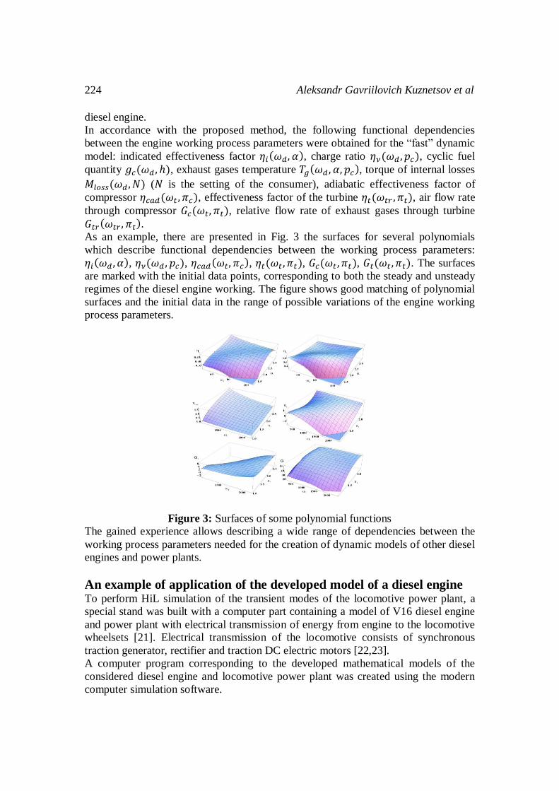
As an example, there are presented in Fig. 3 the surfaces for several polynomials

which describe functional dependencies between the working process parameters:

𝜂𝑖(𝜔𝑑 , 𝛼), 𝜂𝜈(𝜔𝑑 , 𝑝𝑐), 𝜂𝑐𝑎𝑑(𝜔𝑡, 𝜋𝑐), 𝜂𝑡(𝜔𝑡 , 𝜋𝑡), 𝐺𝑐(𝜔𝑡 , 𝜋𝑡), 𝐺𝑡(𝜔𝑡 , 𝜋𝑡). The surfaces

are marked with the initial data points, corresponding to both the steady and unsteady

regimes of the diesel engine working. The figure shows good matching of polynomial

surfaces and the initial data in the range of possible variations of the engine working

process parameters.

Figure 3: Surfaces of some polynomial functions

The gained experience allows describing a wide range of dependencies between the

working process parameters needed for the creation of dynamic models of other diesel

engines and power plants.

An example of application of the developed model of a diesel engine To perform HiL simulation of the transient modes of the locomotive power plant, a

special stand was built with a computer part containing a model of V16 diesel engine

and power plant with electrical transmission of energy from engine to the locomotive

wheelsets [21]. Electrical transmission of the locomotive consists of synchronous

traction generator, rectifier and traction DC electric motors [22,23].

A computer program corresponding to the developed mathematical models of the

considered diesel engine and locomotive power plant was created using the modern

computer simulation software.


A real locomotive electronic control unit with a microprocessor controller which is

the core of hardware part of the booth was connected to computer model of power

plant through an interface device. To verify the developed mathematical models and

to examine control system, HiL simulation of power plant transient process was

performed for the typical operating modes of locomotive. The obtained results of HiL

simulation was then compared to similar experimental processes from the tests of the

real locomotive at the same conditions.

During HiL simulation, the operational control of power plant operating mode and

locomotive motion was performed by the means of computer. The transient processes

of changing the basic parameters of the diesel engine and power plant working

process were displayed on the computer screen in real time. The results of simulation

were saved in the computer memory and then printed as transient processes plots.

Changing the modes during HiL simulation was performed by changing the position

of the locomotive control lever (operator controller). The operator controller had 15

positions, each of them corresponding to different diesel operating modes in

accordance to the locomotive diesel power characteristics. The algorithm of controller

work provides support of diesel power at the value which is set by the operator

control lever. The value of the set power is maintained by two regulators of control

system: regulator of diesel shaft angular velocity and regulator of traction generator

driving system.

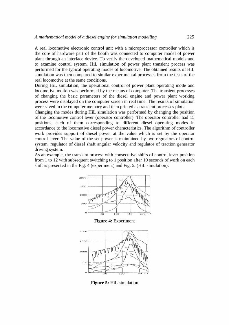
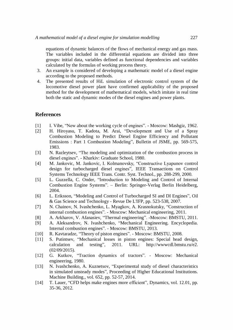
As an example, the transient process with consecutive shifts of control lever position

from 1 to 12 with subsequent switching to 1 position after 10 seconds of work on each

shift is presented in the Fig. 4 (experiment) and Fig. 5. (HiL simulation).

Figure 4: Experiment

Figure 5: HiL simulation


In the experimental and simulated processes, the following parameters characterizing

the working of power plant were fixed: diesel generator shaft angular velocity 𝑛𝑑,

minute-1; turbocharger rotor angular velocity 𝑛𝑡, minute-1; position of fuel quantity

control lever ℎ, mm; limitation of fuel quantity control lever position that is settled by

regulator for different locomotive operator controller lever positions [ℎ], mm;

exccessive pressure of boost air 𝑝𝑐, kPa. In HiL simulation, the current of tractive

generator 𝐼𝑔, A, and voltage 𝑈𝑔, V, are added to those parameters.

Analysis of HiL simulation results and comparison of the calculated processes with

the analogical experimental processes shows that the simulated processes correctly

describe the variation of the primary locomotive power plant parameters with the

predicted error of imitation of dynamic processes less than 10%.

The obtained results confirm applicability of the developed booth and verify

mathematical models on which it based upon. This fact allows using the booth for

HiL simulation of dynamic processes of diesel and locomotive power plant in a wide

range of operating modes and control system settings. Fig. 6 shows HiL simulation

results of controlling process with abrupt shifting of locomotive operator controller

position in sequence of 1-8-15-8-1.

Figure 6

HiL simulation of the transient processes of the locomotive control system yields the

results confirming possibility of applying the proposed method in the development of

complicated models. These models can be used for imitation of the static and dynamic

processes in diesel engines and power plants in real time.

HiL simulation is a very effective means of designing and debugging the engine

control systems. It is advisable to use HiL simulation with proper models of industrial

facilities to adjust and optimize operating modes and working processes.

Conclusion 1. A method of obtaining a mathematical model of a turbocharged diesel engine is

proposed for HiL simulation of the engine control systems. In this method, the

equations of the theory of engine working process along with the functions

based on empirical data are used for calculating the engine parameters in real

time.

2. A turbocharged diesel engine is considered as a set of interacting parts:

cylinders, turbocharger, the intake and exhaust manifolds. Variations of the

output parameters (angular velocities of engine shaft and turbocharger rotor as

well as intake air and exhaust gas pressures) are determined by differential


equations of dynamic balances of the flows of mechanical energy and gas mass.

The variables included in the differential equations are divided into three

groups: initial data, variables defined as functional dependencies and variables

calculated by the formulas of working process theory.

3. An example is considered of developing a mathematic model of a diesel engine

according to the proposed methods.

4. The presented results of HiL simulation of electronic control system of the

locomotive diesel power plant have confirmed applicability of the proposed

method for the development of mathematical models, which imitate in real time

both the static and dynamic modes of the diesel engines and power plants.

References

[1] I. Vibe, “New about the working cycle of engines”. - Moscow: Mashgiz, 1962.

[2] H. Hiroyasu, T. Kadota, M. Arai, “Development and Use of a Spray

Combustion Modeling to Predict Diesel Engine Efficiency and Pollutant

Emissions : Part 1 Combustion Modeling”, Bulletin of JSME, pp. 569-575,

1983.

[3] N. Razleytsev, “The modeling and optimization of the combustion process in

diesel engines”. - Kharkiv: Graduate School, 1980.

[4] M. Jankovic, M. Jankovic, I. Kolmanovsky, “Constructive Lyapunov control

design for turbocharged diesel engines”, IEEE Transactions on Control

Systems Technology IEEE Trans. Contr. Syst. Technol., pp. 288-299, 2000.

[5] L. Guzzella, C. Onder, “Introduction to Modeling and Control of Internal

Combustion Engine Systems”. – Berlin: Springer-Verlag Berlin Heidelberg,

2004.

[6] L. Eriksson, “Modeling and Control of Turbocharged SI and DI Engines”, Oil

& Gas Science and Technology - Revue De L'IFP, pp. 523-538, 2007.

[7] N. Chainov, N. Ivashchenko, L. Myagkov, A. Krasnokutsky, “Construction of

internal combustion engines”. - Moscow: Mechanical engineering, 2011.

[8] A. Arkharov, V. Afanasiev, “Thermal engineering”. -Moscow: BMSTU, 2011.

[9] A. Aleksandrov, N. Ivashchenko, “Mechanical Engineering. Encyclopedia.

Internal combustion engines”. - Moscow: BMSTU, 2013.

[10] R. Kavtaradze, “Theory of piston engines”. - Moscow: BMSTU, 2008.

[11] S. Putintsev, “Mechanical losses in piston engines: Special head design,

calculation and testing”, 2011. URL: http://wwwcdl.bmstu.ru/e2.

(02/09/2015).

[12] G. Kutkov, “Traction dynamics of tractors”. - Moscow: Mechanical

engineering, 1980.

[13] N. Ivashchenko, A. Kuznetsov, “Experimental study of diesel characteristics

in simulated unsteady modes”, Proceeding of Higher Educational Institutions.

Machine Building., vol. 652, pp. 52-57, 2014.

[14] T. Lauer, “CFD helps make engines more efficient”, Dynamics, vol. 12.01, pp.

35-36, 2012.

http://wwwcdl.bmstu.ru/e2


[15] KIVA-4, Los Alamos National Laboratory, 2010. URL:

http://www.lanl.gov/orgs/tt/license/software/kiva/. (02/09/2015).

[16] AVL FIRE, ® Product description, 2014. URL: https://www.avl.com/web/

ast/fire. (02/09/2010).

[17] DIESEL-RK is an engine simulation software. BMSTU, 2014. URL:

http://www.diesel-rk.bmstu.ru. (02/09/2010).

[18] E. Lvovsky, “Statistical methods for constructing empirical formulas”. -

Moscow: Graduate School, 1988.

[19] W. Härdle, “Applied nonparametric methods”. - Tilburg, Netherlands: Center

for Economic Research, Tilburg University, 1992.

[20] Y. Tyurin, A. Makarov, “Analysis of data on the computer”. - Moscow:

INFRA, 2003.

[21] A. Kuznetsov, “A dynamic model of the locomotive power plant”, Bulletin

MSTU. NE Bauman. Mechanical Engineering, vol. 3, pp. 49-56, 2009.

[22] P. Freeland, “Mahle range extender. System and vehicle”, Special Edition.

MAHLE Performance, pp. 8-11, 2013.

[23] S. Sortland, “Hybrid propulsion system for anchor handling tug supply

vessels”, Wärtsilä Technical Journal, vol. 01, pp. 45-48, 2008.

http://www.lanl.gov/orgs/tt/license/software/kiva/

https://www.avl.com/web/ast/fire

https://www.avl.com/web/ast/fire

http://www.diesel-rk.bmstu.ru/

Documents

A mathematical model of a diesel engine for simulation ... · PDF filesimulation of the engine control ... mass in the main parts of the engine. In order to achieve high speed